A Study of Friction Nonlinearity and Compensation for Turntable Servo Systems

Abstract

In view of the worse dynamic performance and steady-state accuracy caused by nonlinear friction in turntable servo systems, challenges are posed in precise positioning tasks. However, most of the existing research ignores the effect of friction on system performance. Therefore, it is of great significance to analyze the nonlinear characteristics of the transmission mechanism and study compensation strategies for improving the control quality of non-direct drive turntable servo systems. Therefore, an improved active disturbance rejection control (ADRC) based on state feedback compensation is proposed in this paper to optimize the accuracy of the turntable servo system and improve the robustness of the system under nonlinear friction conditions. Firstly, friction is modeled and analyzed through offline identification, which is the basis for nonlinear friction compensation. Subsequently, the two methods of friction compensation are compared. Since feedforward compensation is prone to under-compensation and over-compensation, it is highly dependent on the parameters, while the traditional ADRC compensation method has poor dynamic performance under gap conditions. Therefore, the advantages of ADRC and state feedback are combined together to reduce the steady-state error and optimize the control performance of the system. Lastly, the effectiveness of the proposed compensation method is verified and compared through simulations and experiments. The method is able to comprehensively compensate the gap and friction nonlinearities, and the experimental steady-state error is reduced from 0.55° to 1/3 (0.19°), which improves the load-side positioning accuracy. Finally, a conclusion can be drawn that the new compensation method can improve the parameter adjustability, speed estimation precision, and system robustness.

1. Introduction

Friction is a ubiquitous phenomenon in transmission mechanisms, influenced by a multitude of factors, including relative movement speed, external forces, contact surface smoothness, ambient temperature, and the condition of lubricants [1]. The complex interplay of these factors affects the magnitude of frictional forces encountered. Unlike mechanical gaps, friction cannot be mitigated through structural optimization alone, presenting a significant challenge in enhancing the dynamic performance and steady-state accuracy of servo drive systems [2]. Therefore, the accurate modeling of and compensation for friction is crucial in high-precision servo drive systems.

Previous studies have often neglected the impact of friction due to its relatively minor influence under certain conditions. However, during positioning tasks, even small frictional forces can lead to an increase in relative position errors and static friction torque, potentially causing motor stalling [3]. Especially in low-temperature application scenarios, the viscosity of the lubricant medium increases, which in turn increases the frictional torque. To address this issue, a comprehensive approach is adopted, beginning with the offline identification and modeling of the friction characteristics of the experimental platform. This process involves a detailed analysis of the frictional behavior under varying conditions [4].

Since 1519, scholars from various countries have carried out in-depth studies on friction, and various friction characteristics have been summarized over hundreds of years, including (1) static friction; (2) Coulomb friction; (3) Stribeck friction; (4) pre-sliding displacement; (5) variable static friction; (6) friction hysteresis, etc. The first three are static friction characteristics and the last three are dynamic friction characteristics. A friction model was established to reflect the above characteristics.

In 1785, Coulomb made a clear division between static friction and kinetic friction, but the jump of the Coulomb model at zero speed easily leads to instability of the kinetic model. 1866, Reynolds was inspired by the development of fluid dynamics and introduced the concept of viscous hysteresis, which formed the ‘static friction + Coulomb friction + viscous friction’, which is still widely used today. In 1902, Stribeck explored the relationships among relative speed, viscosity, and friction and proposed a smooth exponential curve for the transition from static friction to viscous friction. In 1985, Karnopp’s model was proposed to solve the problems of zero-speed detection and switching between states.

The above models do not reflect the dynamic friction characteristics. In order to reflect the characteristics of pre-slip and variable static friction, Armstrong and Dupont developed a seven-parameter model with three independent equations to describe the friction at each stage, but the identification of its multiple parameters is difficult and the application of the model is limited. Although the seven-parameter model reflects some of the dynamic properties, a truly dynamic model usually requires the introduction of additional state variables to provide more degrees of freedom in the description of the friction characteristics. The earliest dynamic model was proposed by Dahl [5], which introduced the concept of average deformation to describe the pre-slip displacement and frictional hysteresis, but ignored the static friction and Stribeck effect. Haessig and Frieland, from a microscopic point of view, regarded the stochastic behavior of the two contacting surfaces as the contact of a large number of elastic bristles, which is called the bristle model. Subsequently, in order to reduce the complexity of the calculations. The two scholars also proposed an improved reset integral model [6].

Inspired by the average deformation of the bristle model, the Dahl model was extended and the LuGre model was established in [7], which is more complete and easier to implement, making it the most widely used dynamical model. Swevers pointed out that the LuGre model does not describe the hysteresis phenomenon adequately and could not explain the non-local memory problem in the experiments, so he proposed the Leuven model [8], which is the most widely used dynamic model. And Lampaert et al. proposed a generalized Maxwell sliding model based on the Leuven model [9].

Friction compensation is mainly divided into two ideas: friction model-based compensation and non-friction model-based compensation. The essence of the friction model-based compensation strategy is feedforward compensation: the fixed friction model parameters are obtained through offline experiments, or the friction parameters are recognized online through adaptive methods. Then, the friction torque is estimated according to the current state parameters, such as the system speed, and feedforward compensation is carried out. One study [10] used a simple static model (Coulomb + viscous hysteresis) and a Stribeck model for compensation, and the experimental results showed that the latter was more effective. Another study [11] used the LuGre model in the start-up phase and switched to the Stribeck model in the smooth operation phase, which reduced the average speed tracking error to a seventh of the original one. The study by [12] proposed an adaptive friction compensation scheme based on the LuGre model, in which the unknown dynamic parameters and the unmeasurable internal states are obtained by an observer.

The essence of a compensation strategy that is not based on a friction model is to consider the friction as a disturbance in the system, and the disturbance is suppressed by algorithms such as nonlinear proportional integral derivative (PID) control, observer-based control, neural network control, variable structure control, or robust control. The study by [13] estimates the friction effect of a three-wheeled omni-directional mobile robot based on a reduced-order extended state observer, and a large number of experiments demonstrated the effectiveness and robustness of the control method. Since neural networks can approximate any nonlinear function, in the study by [14], an augmented neural network was used to achieve an accurate approximation of the discontinuous function using fewer nodes. Then, an integral sliding mode control was designed based on the system model and the friction model based on the neural network, with the sliding surface as a simple proportional integral function of the positional error, and the control rate obtained by the backpropagation method. The study by [15] improved the tracking response of a DC brushless linear motor by optimally tuning the parameters of a perturbation observer-based variable structure controller using particle swarm optimization (PSO).

From the above literature review, it can be concluded that static friction models allow for easier modeling of friction without overly sacrificing accuracy. The suppression and compensation of unknown friction perturbations can be achieved through the introduction of ADRC. This study delves into the pervasive influence of friction on transmission mechanisms. Friction has a significant effect on fine positioning, leading to increased errors and motor stalls. Therefore, this paper no longer ignores the effect of friction in the transmission link. To address these challenges, a closed-loop structure with state feedback is proposed to compensate for mechanical gaps by enhancing friction through increased surface roughness. Offline identification of friction characteristics with a static friction model is carried out. Feedforward compensation for friction torque is also implemented. Then, an improved linear active disturbance rejection controller (LADRC) is applied with an extended state observer that implements adaptive control to carry out compensation for the unknown dynamic friction and improve the steady-state performance of the system. And the state feedback control implements the composite compensation for gap and friction nonlinearities, which meets the demand of the rotary table servo system for full-operating-condition compensation for nonlinear characteristics. At last, comprehensive simulations and experimental trials validate the effectiveness of the proposed compensation algorithm, showcasing significant enhancements in the system performance.

Compared to previous studies, this paper considers the effect of friction on the transmission link and performs parameter identification under the dual-inertia model to accurately determine the nonlinear parameters, such as friction. On this basis, this paper innovatively combines ADRC with state feedback. The algorithm effectively reduces the steady-state error and improves the control performance.

2. Friction Modeling and Identification

2.1. Friction Modeling

Considering the accuracy of the friction model, the difficulty of parameter identification, and the available experimental conditions, this study selected the widely applied model of “static friction + Coulomb friction + viscous friction.” This model is illustrated in Figure 1, with its mathematical expressions provided in Equation (1). Static friction is the force required to initiate relative motion from rest. When the external force applied is less than the maximum static friction, the static friction force numerically equals the external force; however, when the external force exceeds the maximum static friction, the static friction force is equal to the maximum static friction. Coulomb friction operates under the conditions of non-zero velocity. It is characterized by a frictional force that is dependent on the normal force and the direction of relative motion but is independent of velocity. Viscous friction is a linear model that takes the effects of the lubricating medium into account, where the frictional force is directly proportional to the velocity of the relative motion between objects.

$$T_f=\left\{\begin{array}{l}{T}_e\hspace{0.17em}\hfill \\ T_s\hspace{0.17em}\mathrm{sgn}\hspace{0.17em}(T_e)\hfill \\ T_c\hspace{0.17em}\mathrm{sgn}\hspace{0.17em}(v)+B_{v}V\hfill \end{array}\right.\hspace{1em}\begin{array}{l}V=0,\left|T_e\right|\le T_s\hfill \\ V=0,\left|T_e\right|\hspace{0.17em}>T_s\hfill \\ v\ne 0\hfill \end{array}$$

(1)

In the formula, T_s represents the maximum static friction torque, T_e denotes the external torque (electromagnetic torque), T_c is the Coulomb friction torque, and B_v is the coefficient of viscous friction. The following section identifies these parameters through an offline method.

2.2. Friction Parameter Identification

2.2.1. Introduction to the Identification Algorithm

In this study, the particle swarm optimization (PSO) algorithm is employed for parameter identification. The PSO algorithm is a branch of evolutionary computational methods that seek optimal solutions through iterative processes in a swarm-based approach. As the PSO algorithm converges quickly, occupies less computational space, and can adapt to the needs of complex nonlinear dual-inertia system parameter identification, it was selected to replace the traditional single-inertia parameter identification and optimization algorithm. The principles of PSO are as follows [16]:

M particles exist in a D-dimensional space, and each particle has only two vector attributes: position and velocity. An evaluation function f_m is defined to calculate the distance of each particle from the optimal solution in the space, which is referred to as fitness. By sharing and comparing the fitness of each particle within the current group, the global best solution g_best can be determined. Each particle compares its own fitness and flight experience to determine its current best position p_ibest. The positions and velocities of all particles are then updated, causing each particle to move toward positions with better individual fitness and better group fitness until the optimal solution in the space is reached. The iterative formulas are given in (2).

$$\left\{\begin{array}{l}{x}_i(t+1)=x_i(t)+v_i(t+1)\hfill \\ v_i(t+1)=\gamma v_i(t)+c_1{r}_1[p_{ibest}-x(t)]+c_2{r}_2[g_{best}-x_i(t)]\hfill \end{array}\right.$$

(2)

In Formula (2), the learning factors c₁ and c₂ are both set at 1.7, representing the particle’s self-learning capability and social sharing ability, respectively. Random numbers $r_1$ and r₂ range from 0 to 1. The variables x_i(t) and v_i(t) denote the current position and velocity of the ith particle, respectively, while x_i(t + 1) and v_i(t + 1) represent the position and velocity of the particle at the next time step. The inertia weight $\gamma$ characterizes the confidence level of the particle; a higher value indicates a stronger global search capability and a weaker local search capability. To better balance between the global and local search abilities, Shi et al. proposed the linear decreasing inertia weight (LDIW) [17].

In the friction model, the parameters to be identified include T_c, T_s, and B_v; hence, the dimension of the search space is D = 3. By substituting a particle’s current position and the time series, the identified speed sequence is obtained. The reciprocal of the sum of squared differences between this sequence and the actual speed sequence in the deceleration phase is defined as the particle’s fitness function. Smaller errors indicate stronger particle fitness and a more optimal particle position. The steps for parameter identification using PSO are as follows:

• Randomly initialize the particle population’s initial positions and velocities within the range of dynamic parameters, with a population size of M = 100 and a maximum identification number of 500.
• Evaluate the fitness of each particle, update the personal best and global best values, and retain relatively better parameter identification results.
• Update the particle positions and velocities, forming new identification parameters.
• Repeat iterations until reaching the maximum number of identifications, and select the particle corresponding to the global extremum as the best identification value.

2.2.2. Parameter Identification Experiment

The determination of the maximum static friction torque is presented below:

Under the control mode of i_d* = 0, a slowly increasing q-axis voltage was applied, thereby applying a slowly increasing electromagnetic torque. Considering the hysteresis caused by the motor’s rotational inertia, the relatively stable maximum value of the q-axis current shortly before this moment was identified by examining the electrical current data. This current value was then multiplied by the torque coefficient to calculate the maximum static friction torque. The experiment was repeated, and the average values are reported in

Table 1. Determination of maximum static friction torque.

Number of Experiments	Current Iq (A)	$\mathbf{Maximum} \mathbf{Static} \mathbf{Friction} \mathbf{Torque} {\mathit{T}}_{\mathit{s}}$ (Nm)	$\mathbf{Average} \mathbf{Maximum} \mathbf{Static} \mathbf{Friction} \mathbf{Torque} \overline{{\mathit{T}}_{\mathit{s}}}$ (Nm)
1	0.051	0.041	0.043
2	0.057	0.046
3	0.048	0.038
4	0.069	0.055
5	0.050	0.040
6	0.049	0.039
7	0.053	0.042

.

The determination of the Coulomb friction coefficient and the viscous friction coefficient is shown below:

With a given q-axis voltage signal of U_q = 10 V, after the motor had operated stably for a period, the power supply was cut off and the motor circuit was opened to allow it to decelerate freely without the influence of back electromotive force (EMF). Disregarding the minimal currents, the motion equation of the motor at this point is:

$$J_m{\ddot{\theta }}_m=-T_g-(T_c+B_v{\ddot{\theta }}_m)$$

(3)

The variables in (3) are explained in Figure 2. In a dual-inertia system, $T_c$ is the Coulomb friction moment, $B_v$ is the viscous friction coefficient, $J_m$ is the motor inertia on the drive side, ${\theta }_m$ is the motor angle on the drive side, and $T_g$ denotes the axial torque component, a variable that is specific to a dual-inertia system and whose mathematical expression is shown in Figure 2.

It is posited that the torque equals the moment of inertia on the load side. In this experimental setup, the inertia of the motors on both the drive and load sides are equal; therefore, (3) is revised to (4).

$$2J_m{\ddot{\theta }}_m=-(T_c+B_v{\ddot{\theta }}_m)$$

(4)

A solution to the differential equation provides the time expression for the motor’s rotational speed.

$${\dot{\theta }}_m=-{\displaystyle \frac{T_c}{B_v}}+({\displaystyle \frac{T_c}{B_v}}+{\theta }_0)e^{-\hspace{0.17em}{\displaystyle \frac{B_v}{2J_m}}t}$$

(5)

Through two repeated experiments, the relationship between the motor speed and time during the power-off deceleration process was measured, and its curve was fitted by PSO. The results are shown in Figure 3. The coefficients were calculated by bringing the above test results into Equation (5). And these coefficients were deformed to obtain the parameters to be identified. Let the identification coefficients T_c/B_v, θ₀, and B_v/J_m be denoted as a, b, and c, respectively. The formula for solving the friction parameters is given in (6), and the results are presented in

Table 2. Measurement of friction torque characteristic parameters.

Experimental Trials	Coulomb Friction Torque, Tc (Nm)	Viscous Friction Coefficient, Bv (Nm/(rad/s))
1	$2.098\times {10}^{-2}$	$6.903\times {10}^{-4}$
2	$2.121\times {10}^{-2}$	$6.979\times {10}^{-4}$
Average value	$2.110\times {10}^{-2}$	$6.941\times {10}^{-4}$

.

$$\left\{\begin{array}{c}{B}_v=c{J}_m\\ T_c=ac{J}_m\end{array}\right.$$

(6)

At the same time, the above experiments also proved that, when the number of iterations was below 20, the optimal fitness decreased as the number of iterations increased; and after the number of iterations exceeded 20, the optimal fitness tended to be close to 0, indicating that the iterative computation of the PSO accomplished its fitting objective. Therefore, the number of iterations for PSO was set to be 20.

3. Compensation Based on the Friction Model

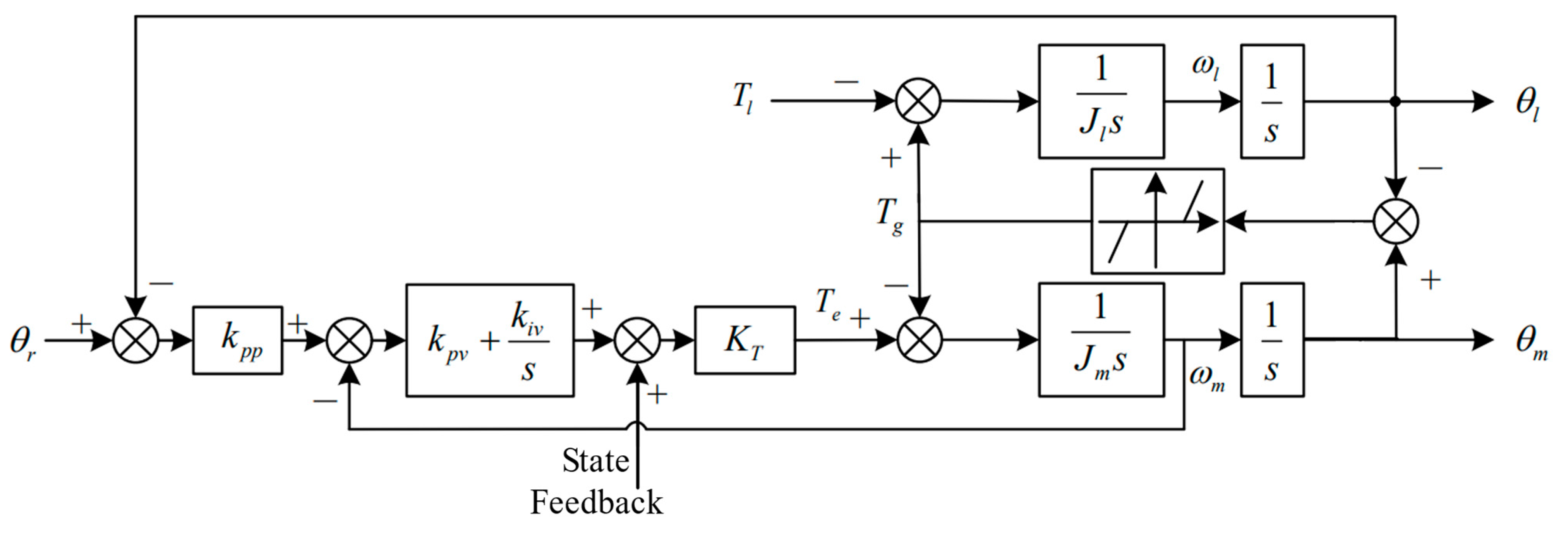
3.1. Feedforward Compensation Based on the Friction Model

The principle of feedforward compensation is relatively straightforward: following accurate modeling of the system’s friction, the friction model is combined with the system’s state variables to compute the friction torque, which is then fed forward to the controller for compensation. In the simulation model, friction is added; the effectiveness of the compensation is shown in Figure 4. This method does not affect the stability of the system; however, it is dependent on the accuracy of the model. When parameters change due to environmental factors or operational conditions, the parameters identified from offline experiments may become inaccurate, leading to under-compensation or over-compensation. For example, with T_c’ = 1.5T_c, over-compensation causes oscillation in the position of the load.

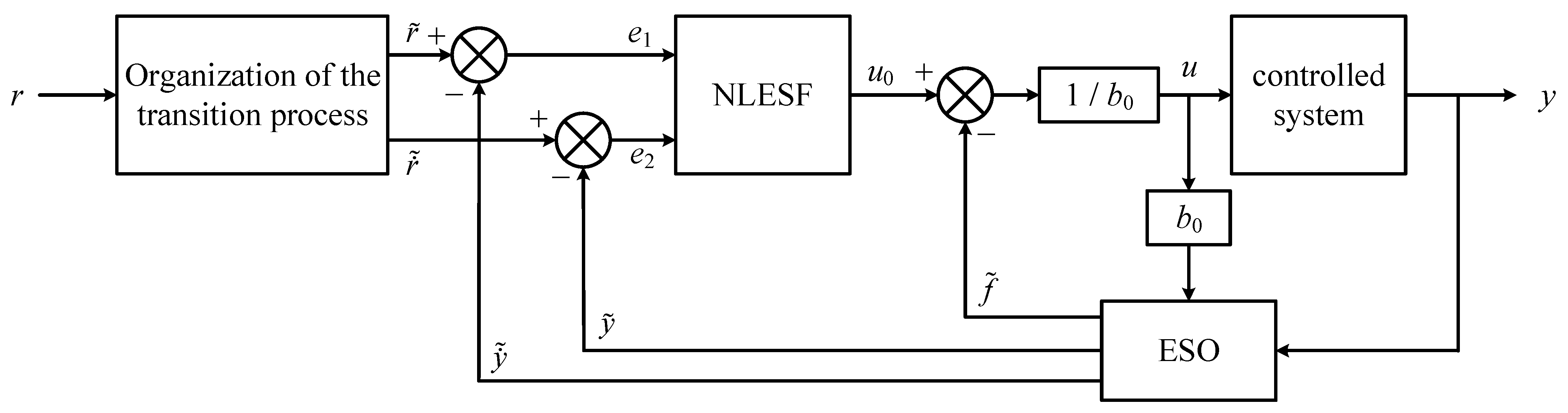
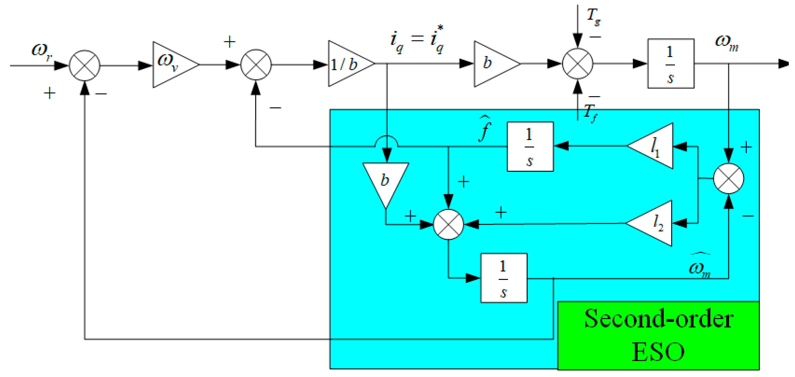
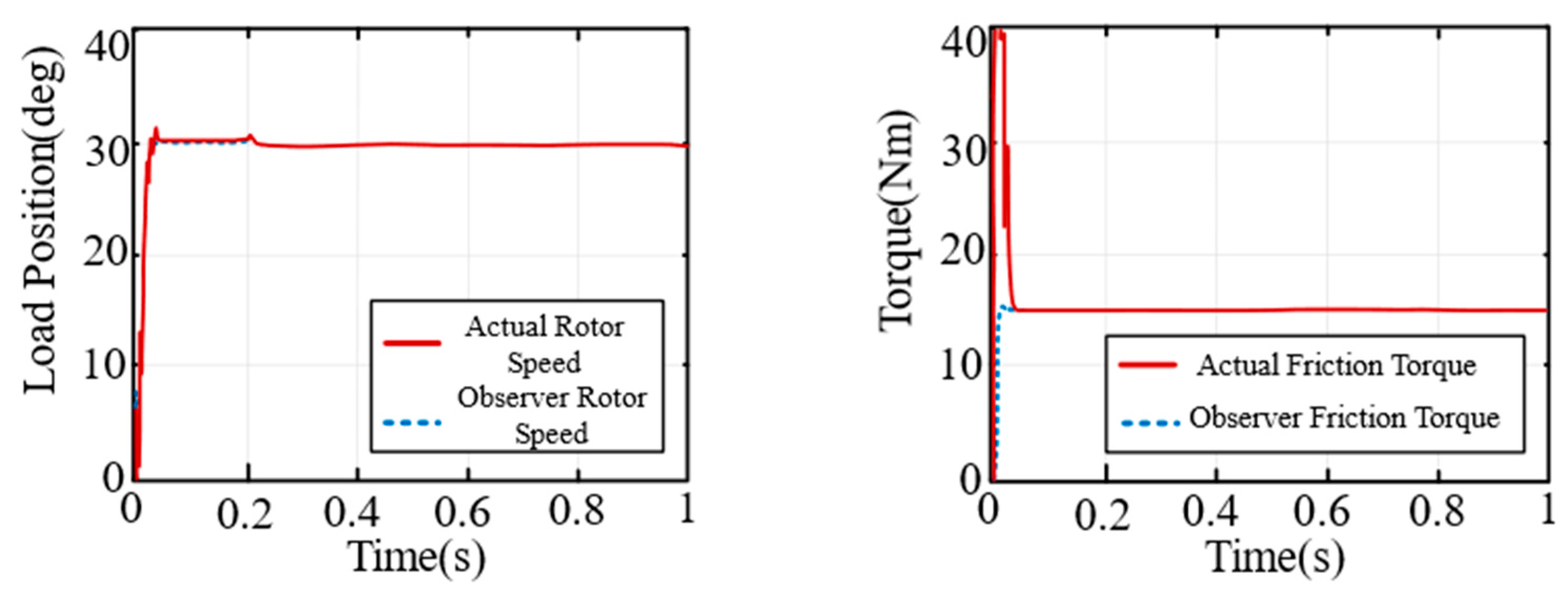
3.2. Friction Compensation Based on Extended State Observer

In this research, the subject was a dual-inertia servo system, where the parameters of the friction model are either difficult to obtain or subject to variability. Considering friction as a disturbance, it was estimated and compensated through the use of a state observer.

In recent years, active disturbance rejection control (ADRC) has been extensively studied and applied as an algorithm that does not depend on precise models and can effectively address system disturbances [18]. The core idea of ADRC is to conceptualize all uncertainties affecting the controlled system as the “total disturbance”. This disturbance is then expanded into the system states and estimated in real-time through an extended state observer (ESO), the typical structure of which is depicted in Figure 5. The tracking differentiator (TD) plays a crucial role by enabling rapid and overshoot-free tracking of input signals, providing differential signals, and managing transition processes to prevent control saturation due to excessively large reference signals. The extended state observer is a significant component within ADRC, tasked with observing the output and its derivatives. The nonlinear state error feedback control law (NLESF) combines the errors of the extended states nonlinearly to derive the control values.

Traditional ADRC is characterized by its minimal disturbance estimation error and rapid dynamic response. However, it encounters difficulties in parameter tuning and features complex nonlinear functions. For instance, ADRC utilizes the fast synthetic control function, fhan, for discretization to achieve swift tracking and differentiation while avoiding high-frequency oscillations; it also employs the fal power function to establish a nonlinear feedback control law. The expressions for both functions, as shown in (7), are relatively complex. Therefore, this project adopted the linear ADRC (LADRC) approach proposed by the team led by Gao Zhiqiang [19].

$$\left\{\begin{array}{l}fhan=-\left\{\begin{array}{c}rsign(a),\left|a\right|>d\hfill \\ r{\displaystyle \frac{a}{d}}\hspace{0.17em}\hspace{0.17em}\hspace{0.17em}\hspace{0.17em}\hspace{0.17em}\hspace{0.17em}\hspace{0.17em}\hspace{0.17em}\hspace{0.17em}\hspace{0.17em}\hspace{0.17em},\left|a\right|\hspace{0.17em}\le d\end{array}\right.\hfill \\ fal=\left\{\begin{array}{l}{\displaystyle \frac{x}{{\eta }^{1-\alpha }}}\hspace{0.17em}\hspace{0.17em}\hspace{0.17em}\hspace{0.17em}\hspace{0.17em}\hspace{0.17em}\hspace{0.17em}\hspace{0.17em}\hspace{0.17em}\hspace{0.17em}\hspace{0.17em}\hspace{0.17em}\hspace{0.17em}\hspace{0.17em},\left|x\right|\hspace{0.17em}<\hspace{0.17em}\eta \hfill \\ |x{|}^{\alpha }\hspace{0.17em}sign(x),|x|\hspace{0.17em}\ge \hspace{0.17em}\eta \hfill \end{array}\right.\hfill \end{array}\right.$$

(7)

In Equation (7), r represents the rate factor, which determines the response speed of the differentiator; a and d are mathematical expressions for control compensation and the rate factor and do not possess practical significance; x denotes the error or the error differential signal; α and η are adjustable parameters of the controller, and they also do not have practical significance.

To simplify the analysis, the initial consideration focused on the no-load steady-state phase where the steady-state torque was zero. The expression for the controlled object is as follows:

$$\begin{array}{l}\dot{\omega }={\displaystyle \frac{1}{J_m}}[K_T(i_q+i_{comp})-T_f]\hfill \\ \hspace{0.17em}\hspace{0.17em}\hspace{0.17em}={\displaystyle \frac{K_T}{J_m}}{i}_q+{\displaystyle \frac{1}{J_m}}[K_T{i}_{comp}-T_f]=b{i}_q+f\hfill \end{array}$$

(8)

The selection of the system state variables is as follows:

$$\dot{x}=\left[\begin{array}{c}{\dot{\omega }}_m\\ \dot{f}\end{array}\right]=\underset{A}{\underbrace{\left[\begin{array}{cc}0& 1\\ 0& 0\end{array}\right]}}\underset{x}{\left[\begin{array}{c}{\omega }_m\\ f\end{array}\right]}+\underset{B}{\left[\begin{array}{c}b\\ 0\end{array}\right]i_q}+\left[\begin{array}{c}0\\ 1\end{array}\right]\dot{f}$$

(9)

The selection of the output variables is as follows:

$$y={\omega }_m=\underset{c}{\left[\begin{array}{cc}1& 0\end{array}\right]}\underset{x}{\left[\begin{array}{c}{\omega }_m\\ f\end{array}\right]}$$

(10)

The design of the second-order ESO observer is as follows.

$$\left\{\begin{array}{l}\dot{\widehat{x}}=A\widehat{x}+Bu+L(y-\widehat{y})\Rightarrow \left[\begin{array}{c}{\dot{\widehat{\omega }}}_m\\ \dot{\widehat{f}}\end{array}\right]=\underset{A}{\underbrace{\left[\begin{array}{cc}0& 1\\ 0& 0\end{array}\right]}}\left[\begin{array}{c}{\omega }_m\\ f\end{array}\right]+\underset{B}{\left[\begin{array}{c}b\\ 0\end{array}\right]}{i}_q+\underset{L}{\left[\begin{array}{c}{l}_1\\ l_2\end{array}\right]}\left[\begin{array}{c}{\omega }_m-{\widehat{\omega }}_m\\ f-\widehat{f}\end{array}\right]\hfill \\ \widehat{y}=C\widehat{x}\Rightarrow {\widehat{\omega }}_m=\underset{c}{\left[\begin{array}{cc}1& 0\end{array}\right]}\left[\begin{array}{c}{\widehat{\omega }}_m\\ \widehat{f}\end{array}\right]\hfill \end{array}\right.$$

(11)

In Equation (11), $L(y-\widehat{y})$ represents the correction error term. Let the state estimation error be $\tilde{x}=x-\widehat{x}$. By combining (9), (10), and (11), the state error equation can be derived.

$${\displaystyle \frac{d\tilde{x}}{dt}}=\dot{x}-\dot{\widehat{x}}=(A-LC)\tilde{x}+\left[\begin{array}{c}0\\ 1\end{array}\right]\dot{f}$$

(12)

In the equation above, if f is bounded, then when the matrix (A – LC) is a Hurwitz matrix (where all the roots of the polynomial have negative real parts), the observation error remains bounded [20]. By setting the characteristic polynomial in the form of (13) to ensure that all characteristic roots are in the left half-plane, the parameters are given as l₁ = 2ω₀ and l₂ = ω₀², where ω₀ represents the bandwidth of the observer. A higher ω₀ reduces the observation error but amplifies the impact of noise; conversely, a lower ω₀ results in a delay in the overall disturbance observation. In this study, ω₀ = 500 rad/s.

$$\left|sI-(A-LC)\right|=\left|\begin{array}{cc}s+l_1& -1\\ l_2& s\end{array}\right|=s^2+l_{1}s+l_2={(s+{\omega }_o)}^2$$

(13)

In the control law designed (14), ω_v represents the desired bandwidth of the speed loop. For this study, ω_v is set at 100 rad/s.

$$i_{q0}={\omega }_v({{\omega }_r}^{*}-{\widehat{\omega }}_m)$$

(14)

When the input is controlled in the form of (15), the output satisfies (16).

$$i_q={\displaystyle \frac{i_{q0}-\widehat{f}}{b}}$$

(15)

$${\dot{\omega }}_m=b{i}_q+f=i_{q0}-\widehat{f}+f\cong i_{q0}$$

(16)

A simulation was conducted on the speed loop control based on the second-order extended state observer (ESO), aiming to assess the disturbance observation effects. The control diagram is depicted in Figure 6. Under no-load conditions, a step speed command of ω_r* = 30 rad/s was applied. It was observed that the motor speed was able to track the actual speed, stabilizing around 0.2 s after an overshoot. The friction torque, as an expanded state variable, eventually converged to the actual value. However, during the speed ramp-up phase, the observed values failed to track the real-time changes in friction torque. For applications requiring high dynamic response, it might be beneficial to also treat the dynamic response as an expanded state in the system, thus increasing the order of the ESO to reduce the observation error [21].

Replacing the speed loop PI controller with the aforementioned LADRC speed loop controller yielded discernible changes in the system dynamics. Upon imposing a predefined ramp position input, the system response, depicted in Figure 7, exhibited oscillations in the load position. The subsequent elimination of oscillatory behavior through clearance adjustment to zero underscores its pivotal role in system stabilization. These simulation findings highlight the diminished efficacy of the state feedback compensation algorithm for clearance after the adoption of the LADRC speed loop controller instead of the PI speed regulator.

According to (8), the state feedback compensation current, icomp, is categorized as part of the total disturbance and is eliminated via feedforward compensation by the LADRC controller. An improved LADRC controller configuration is depicted in Figure 8a, where its output includes the compensation current. In Figure 8b, both the load position and speed are stable, with no oscillations observed.

However, the introduction of a state feedback compensation current also results in a steady-state offset, and due to the adjustments made by the speed loop controller, the original steady-state error formula is no longer applicable, though it can still provide useful insights. A comparison between the two-speed loop controllers reveals that changes in gain are crucial in influencing the steady-state error.

The transfer function of the control output and the given input for LADRC is expressed as follows:

$$k_{pv}={\displaystyle \frac{{\omega }_v}{b_0}}$$

(17)

The expression for the steady-state error was revised to (19). Additionally, another revision indicates that the steady-state error under load conditions is independent of the load torque T_l. This independence arises because when utilizing the improved LADRC speed loop controller, the ADRC feedforward negates the influence of the non-zero shaft torque T_g caused by the load torque. Consequently, this does not affect the feedback coefficient k₁.

$$e=\left\{\begin{array}{l}{b}_0{\displaystyle \frac{k_1(-\epsilon )}{k_{pp}{\omega }_v}}\hfill \\ b_0{\displaystyle \frac{k_1(T_l/K+\epsilon )}{k_{pp}{\omega }_v}}\hfill \end{array}\right.\begin{array}{l}\begin{array}{l}No\hspace{0.17em}Load\hfill \\ \hspace{0.17em}\hfill \end{array}\hfill \\ Carrying\hspace{0.17em}Load\hfill \end{array}$$

(18)

4. Simulation and Experimental Validation of Friction Compensation

On the basis of the theoretical analysis above, a simulation and experimental model was built. The motor parameters used in the simulation are shown in

Table 3. Motor parameters used in the simulation.

Parameter	Numerical Value
Rated power (W)	750
Rated current (A)	3
Rated torque (Nm)	2.39
Number of pole pairs	5
$\mathrm{Moment} \mathrm{of} \mathrm{inertia} (\mathrm{k}\mathrm{g}·{\mathrm{m}}^2$)	$1.82\times {10}^{-4}$

. An experimental platform of pair drag was built to verify the friction characteristics and its compensation algorithm, and it is shown in Figure 9.

4.1. Simulation and Experimental Validation

At 0.5 s, a 90-degree step position signal was introduced. Subsequent analysis delineated the system responses and friction torque manifestations under varying conditions, specifically the no-load and 20% rated load scenarios, which are presented in Figure 10 and Figure 11. Notably, the incurred steady-state errors amounted to 0.01° and 0.001°, respectively. This observation result underscores the mitigative influence of loading on the system, a phenomenon corroborated by prior scholarly discourse. The utilization of a second-order extended state observer (ESO) engenders a discernible delay in the observation of friction torque, a feature congruent with theoretical conjecture.

By altering the friction parameter to T_c′ = 1.5T_c, the system’s response and the observation of the friction torque are illustrated in Figure 12. The steady-state error of 0.0055° indicates that the compensation algorithm remained effective even when the friction varied over time. Figure 13 compares the system responses of two control methods when there was a mismatch in the friction parameters. Utilizing only “PI control + state feedback control” resulted in a steady-state error of 0.34° due to the absence of a friction model’s feedforward compensation. In contrast, when employing “enhanced LADRC + state feedback control”, the steady-state error was significantly reduced to just 0.014°.

A 90° step position signal was applied at 0.5 s, and Figure 14 compares the load positions before and after compensation. The maximum steady-state errors were 0.19° and 0.55°, respectively, indicating an improvement in the positioning accuracy.

4.2. Discussion of Simulation and Experiment

(1).

From the comparison of Figure 10 and Figure 11, it can be seen that load had a calming effect on the system. Due to the second-order ESO used, the friction torque observation shows hysteresis, which is in line with the expected theoretical analysis.

(2).

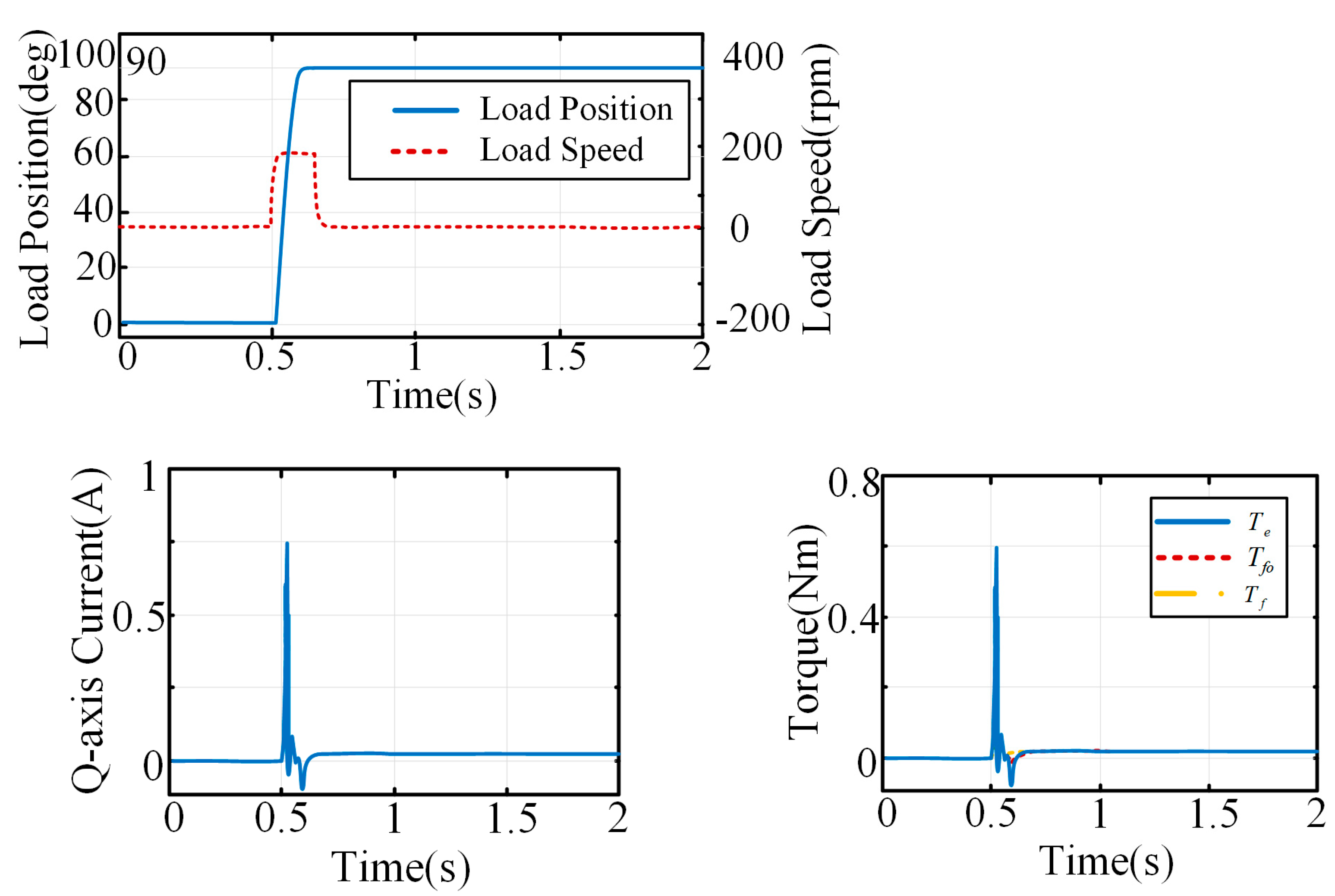
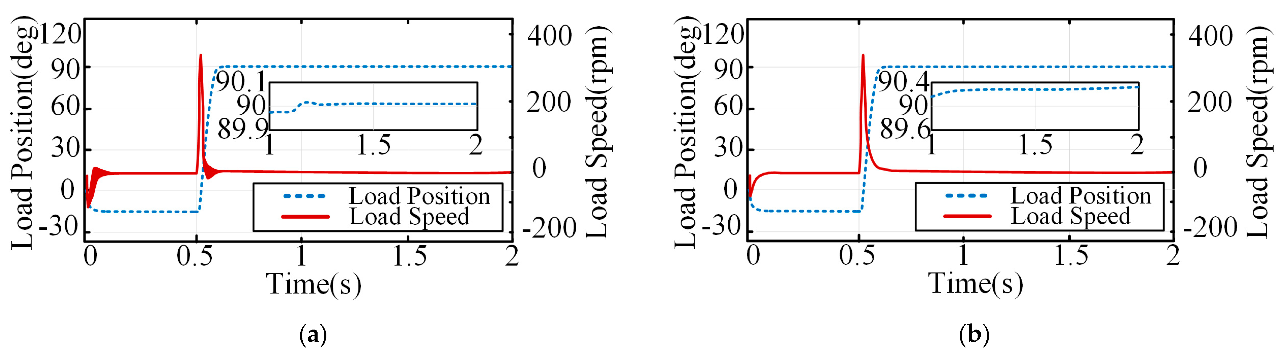
As shown Figure 12, the friction parameters were varied and the system steady-state error was smaller, indicating that the compensation algorithm was equally effective in the case of time-varying friction.

(3).

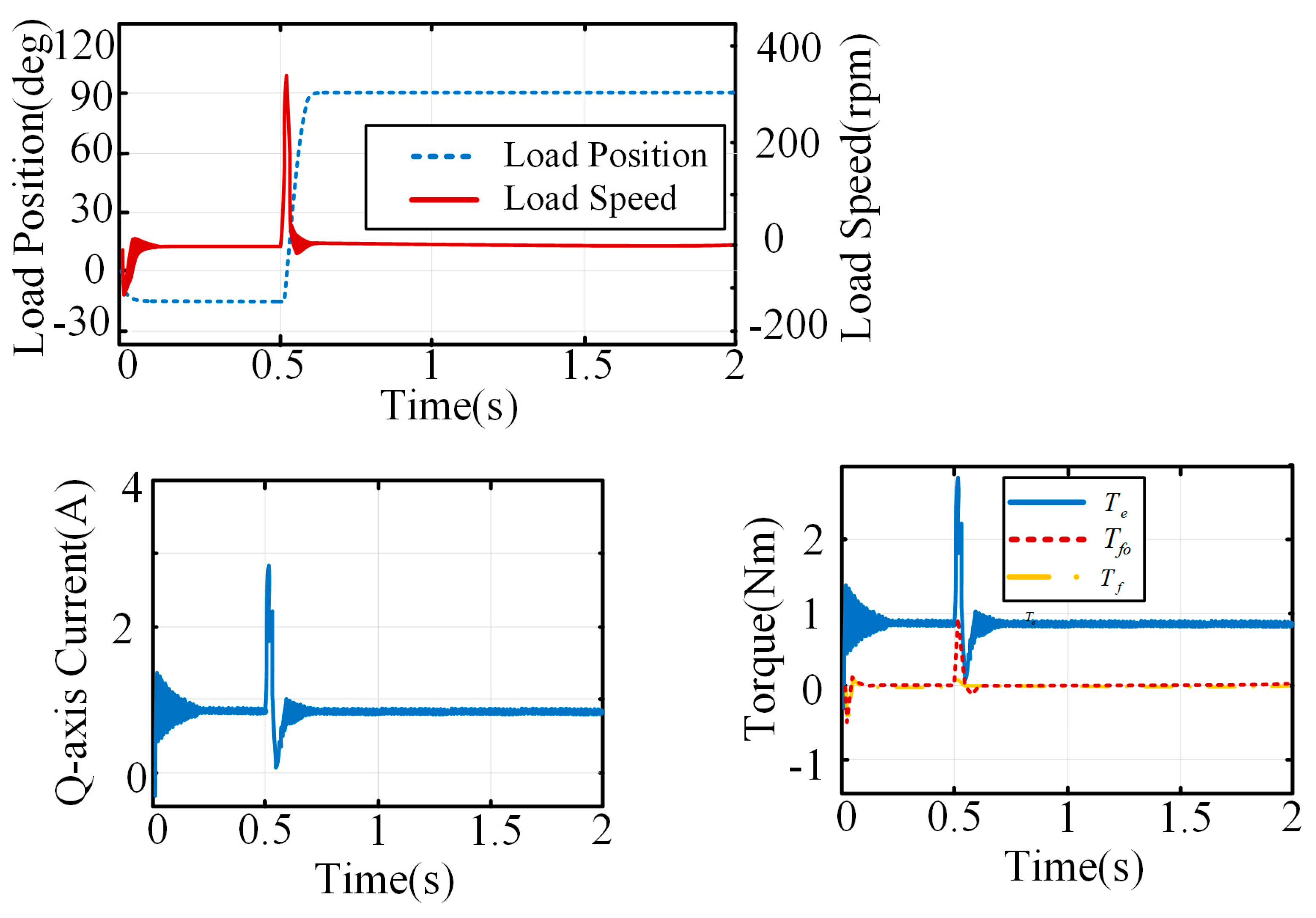
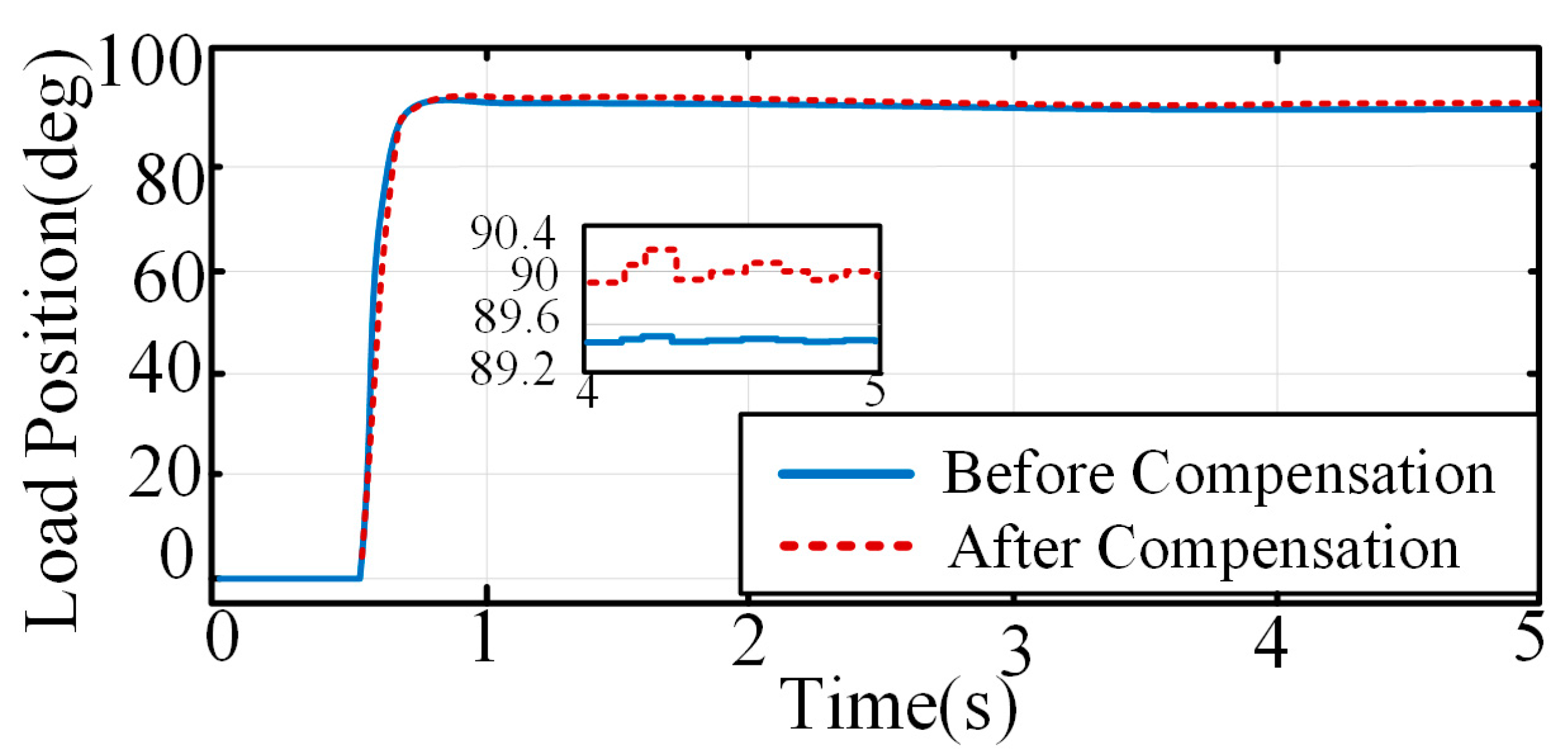
As shown in Figure 13, when the friction parameters were not matched, the friction model feedforward compensation was added by the improved “LADRC + state feedback control”, and the steady-state error was much smaller than that of the “PI control + state feedback control”, which proves the effectiveness of the proposed new algorithm compared to the traditional PI control.

5. Conclusions

In this paper, the parameters of maximum static friction, Coulomb friction, and viscous friction of a friction model were first identified offline based on the particle swarm algorithm, and the feedforward compensation algorithm based on the model was validated through simulation, which was found to be prone to an over/under-compensation phenomenon when the parameters were not matched.

In order to realize the adaptive compensation, the friction disturbance torque was observed by using the second-order dilated state observer. Due to the deterioration of the dynamic response performance of the conventional ADRC controller in the presence of a gap, it could not meet the demand of control performance.

Therefore, the performance of ADRC was improved by combining it with the state feedback method, and the improved controller gain was calculated to correct the steady-state static differential equation.

The simulations and experiments showed that this method was able to compensate for the gap and friction nonlinearity in an integrated way, and the following conclusions are drawn:

(1).

Feedforward compensation based on a friction model is highly dependent on the accuracy of parameter identification, and inaccuracies in the motor parameters trigger system oscillations.

(2).

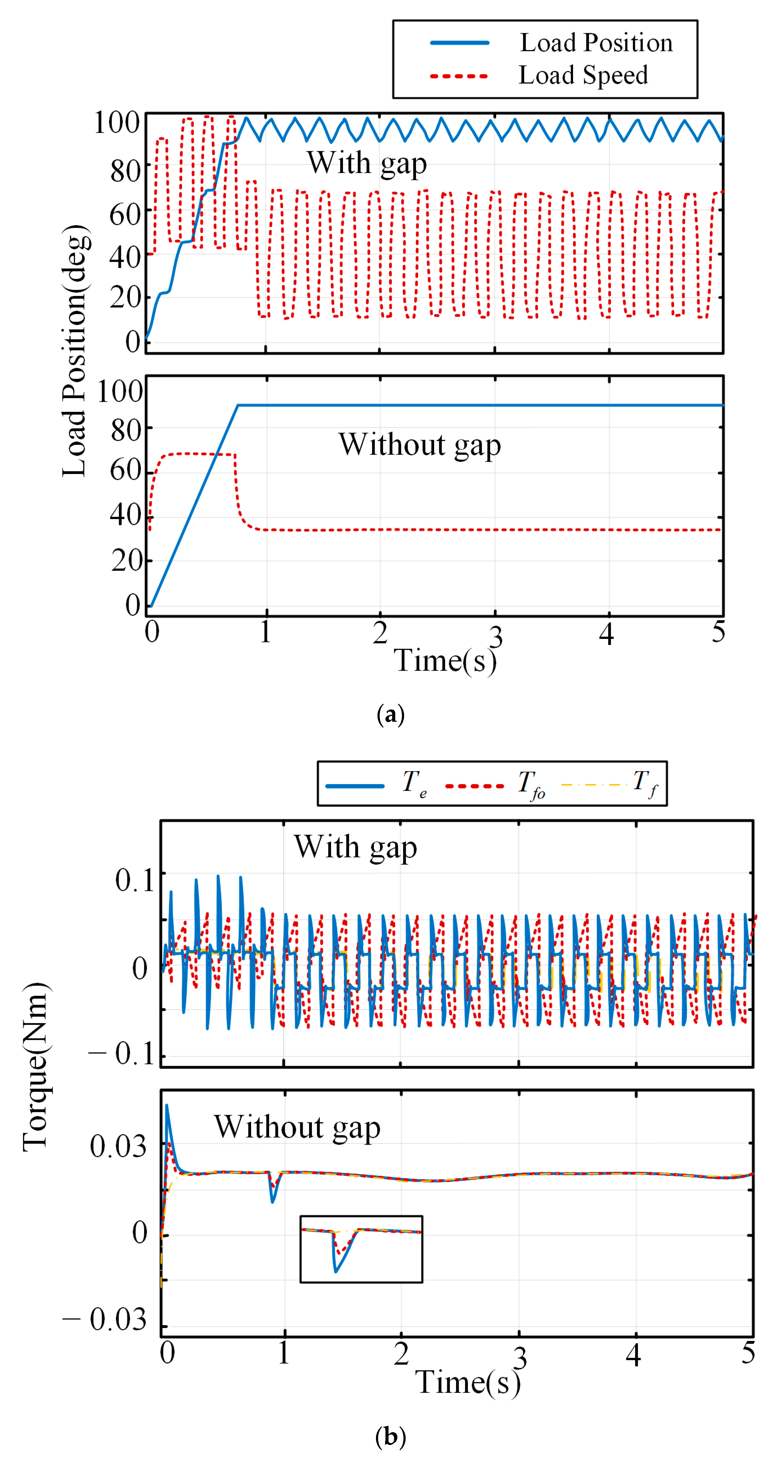
With the application of the traditional ADRC algorithm in friction compensation, a small steady-state error and a rapid dynamic response can be reached. However, the compensation effect of the gap is not obvious, and the dynamic performance is seriously degraded when there is a gap in the transmission mechanism.

(3).

Introducing state feedback compensation on the basis of the traditional ADRC can effectively improve the positioning accuracy of the load side of the transmission system. The experimental steady state error was reduced from 0.55° to 1/3 (0.19°) after compensation. Moreover, the robustness of the improved compensation algorithm to the parameters is further improved for different load conditions.

Due to the experimental conditions, the dynamic model was not chosen to describe the friction in this project. In subsequent research, the friction can be described more accurately based on the dynamic model, and the suppression algorithm of the friction disturbance can be further improved on this basis to obtain a better suppression effect.

References

1. Yu, H.; Gao, H.; Deng, H.; Yuan, S.; Zhang, L. Synchronization Control with Adaptive Friction Compensation of Treadmill-based Testing Apparatus for Wheeled Planetary Rover. IEEE Trans. Ind. Electron. 2022, 69, 592–603. [Google Scholar] [CrossRef]
2. Véronneau, C.; Denis, J.; Lhommeau, P.; St-Jean, A.; Girard, A.; Plante, J.S.; Bigué, J.P.L. Modular Magnetorheological Actuator with High Torque Density and Transparency for the Collaborative Robot Industry. IEEE Robot. Autom. Lett. 2023, 8, 896–903. [Google Scholar] [CrossRef]
3. Thenozhi, S.; Concha, A.; Resendiz, J.R. A Contraction Theory-based Tracking Control Design with Friction Identification and Compensation. IEEE Trans. Ind. Electron. 2022, 69, 6111–6120. [Google Scholar] [CrossRef]
4. Qian, X.; Peiliang, W.; Zuxin, L. Parameter identification of permanent magnet servo system based on recursive least squares method. J. Electrotechnol. 2016, 31, 9. [Google Scholar]
5. Liu, C.; Luo, G.; Duan, X.; Chen, Z.; Zhang, Z.; Qiu, C. Adaptive LADRC-Based Disturbance Rejection Method for Electromechanical Servo System. IEEE Trans. Ind. Appl. 2020, 56, 876–889. [Google Scholar] [CrossRef]
6. Zhou, Z.; Guo, R. A Disturbance-Observer-Based Feedforward-Feedback Control Strategy for Driveline Launch Oscillation of Hybrid Electric Vehicles Considering Nonlinear Backlash. IEEE Trans. Veh. Technol. 2022, 71, 3727–3735. [Google Scholar] [CrossRef]
7. Wang, G.; Liu, R.; Zhao, N.; Ding, D.; Xu, D. Enhanced linear ADRC strategy for HF pulse voltage signal injection based sensorless IPMSM drives. IEEE Trans. Power Electron. 2019, 34, 514–525. [Google Scholar] [CrossRef]
8. Liang, L.H.; Wang, L.Y.; Wang, J.F. Energy-Saving Nonlinear Friction Compensation Method for Direct Drive Volume Control Flange-Type Rotary Vane Steering Gear. IEEE Access 2019, 7, 148351–148362. [Google Scholar] [CrossRef]
9. Papadopoulos, E.G.; Chasparis, G.C. A Novel Friction Compensation Method Based on Stribeck Model With Fuzzy Filter for PMSM Servo Systems. IEEE Trans. Ind. Electron. 2023, 70, 12124–12133. [Google Scholar]
10. Ahi, B.; Nobakhti, A. Hardware Implementation of an ADRC Controller on a Gimbal Mechanism. IEEE Trans. Control Syst. Technol. 2018, 26, 2268–2275. [Google Scholar] [CrossRef]
11. Song, Z.; Mei, X.; Jiang, G. Inertia Identification based on Model Reference Adaptive System with Variable Gain for AC Servo Systems. In Proceedings of the International Conference on Mechatronics and Automation (ICMA), Takamatsu, Japan, 6–9 August 2017; pp. 188–192. [Google Scholar]
12. Ren, C.; Li, X.; Yang, X.; Ma, S. Extended State Observer based Sliding Mode Control of an Omnidirectional Mobile Robot with Friction Compensation. IEEE Trans. Ind. Electron. 2019, 66, 9480–9489. [Google Scholar] [CrossRef]
13. Ming, M.; Liang, W.; Ling, J.; Feng, Z.; Al Mamun, A.; Xiao, X. Composite Integral Sliding Mode Control with Neural Network-based Friction Compensation for a Piezoelectric Ultrasonic Motor. In Proceedings of the Annual Conference of the IEEE Industrial Electronics Society (IECON), Singapore, 18–21 October 2020; pp. 4397–4402. [Google Scholar]
14. Tian, Y.-C.; Huang, S.; Liang, W.; Tan, K.K. Intelligent friction compensation: A review. IEEE/ASME Trans. Mechatron. 2019, 24, 1763–1774. [Google Scholar]
15. Cui, N.; Zhang, Q.; Li, G. Servo rotary table friction modelling and compensation based on switching system theory. Micromotor 2019, 52, 6. [Google Scholar]
16. Sun, L.; Li, X.; Chen, L.; Shi, H.; Jiang, Z. Dual-Motor Coordination for High-Quality Servo with Transmission Backlash. IEEE Trans. Ind. Electron. 2023, 70, 1182–1196. [Google Scholar] [CrossRef]
17. Wang, Y.; Wu, Z.; Xue, Y.; Li, D.; Li, Z. Design of linear self-immunity controller for high-order large-inertia systems. Control Decis. 2023, 38, 999–1007. [Google Scholar]
18. Yang, M.; Ni, Q.; Liu, X.; Xu, D. Vibration suppression and over-quadrant error mitigation methods for a ball-screw driven servo system with dual-position feedback. IEEE Access 2020, 8, 213758–213771. [Google Scholar] [CrossRef]
19. Beerens, R.; Bisoffi, A.; Zaccarian, L.; Nijmeijer, H.; Heemels, M.; van de Wouw, N. Reset PID design for motion systems with Stribeck friction. IEEE Trans. Control. Syst. Technol. 2022, 30, 294–310. [Google Scholar] [CrossRef]
20. Yang, M.; Qu, W.Y.; Chen, Y.Y. Online inertia identification of servo system based on variable period recursive least squares and Kalman observer. J. Electrotechnol. 2018, 33, 367–376. [Google Scholar]
21. Bu, F.; Yang, Z.; Gao, Y.; Pan, Z.; Pu, T.; Degano, M.; Gerada, C. Speed Ripple Reduction of Direct-Drive PMSM Servo System at Low-Speed Operation Using Virtual Cogging Torque Control Method. IEEE Trans. Ind. Electron. 2021, 68, 160–174. [Google Scholar] [CrossRef]
Figure 1. Static friction + Coulomb friction + viscous friction model.
Applsci 14 08002 g001
Figure 2. Schematic diagram of each variable in a dual-inertia system.
Applsci 14 08002 g002
Figure 3. Curve fitting and iterative optimization of free deceleration. (a) Experiment 1. (b) Experiment 2.
Applsci 14 08002 g003
Figure 4. Feedforward compensation based on friction modeling.
Applsci 14 08002 g004
Figure 5. Block diagram of the classical structure of active disturbance rejection control.
Applsci 14 08002 g005
Figure 6. Motor speed loop control based on LADRC.
Applsci 14 08002 g006aApplsci 14 08002 g006b
Figure 7. System response with LADRC loop controller. (a) Load position and rotational speed. (b) Friction torque, observed torque, and electromagnetic torque.
Applsci 14 08002 g007
Figure 8. Block diagram of improved LADRC speed loop control and system response. (a) Control block diagram. (b) Load position and rotation speed.
Applsci 14 08002 g008
Figure 9. Experimental platform.
Applsci 14 08002 g009
Figure 10. System response and friction torque measurement under no-load conditions.
Applsci 14 08002 g010
Figure 11. System response and friction torque observation at 20% rated load conditions.
Applsci 14 08002 g011
Figure 12. System response and friction torque observation at 20% rated load with a friction parameter of Tc’ = 1.5Tc.
Applsci 14 08002 g012
Figure 13. System responses of the two control methods when the friction parameters are mismatched. (a) Improved LADRC control + state feedback control. (b) PI control + state feedback control.
Applsci 14 08002 g013
Figure 14. Comparison of load position before and after compensation.
Applsci 14 08002 g014