Abstract
This work studies how the Elo rating system can be applied to score-based sports, where it is gaining popularity, and in particular for predicting the result at any point of a game, extending its statistical basis to stochastic processes. We derive some new theoretical results for this model and use them to implement Elo ratings for basketball and soccer leagues, where the assumptions of our model are tested and found to be mostly accurate. We showcase several metrics for comparing the performance of different rating systems and determine whether adding a feature has a statistically significant impact. Finally, we propose an Elo model based on a discrete process for the score that allows us to obtain draw probabilities for soccer matches and has a performance competitive with alternatives like SPI ratings.
1. Introduction
Rating systems track and predict the performance of competitors in pairwise zero-sum games. They were initially developed to objectively measure the strength of chess players, with the first successful system proposed by Arpad Elo in 1960 and adopted by the United States Chess Federation (USCF) to replace the more problematic Harkness rating system. The International Chess Federation (FIDE) also started publishing ratings of its players in 1970 and continues to publish them today. The Elo rating system, or variants of it, are also used by most chess websites, where users are automatically matched against other players of similar strength, as well as by federations of Go and Scrabble players, and several video games.
The motivation, mathematical basis, and problems of the Elo rating system are explained in detail in Elo’s book [1], and the academic literature is summarized in [2]. The system gives each player a real parameter called their rating and defines an algorithm to update it with the result of each new game. Winning a game increases the player’s rating, and losing decreases it, but the increase depends on the rating of the rival. This allows for the ratings to change as the strength of the players also does. More sophisticated systems like glicko, proposed by Mark Glickman [3], include two parameters for each player, representing the strength and its variability, to allow for players gaining strength more quickly than others.
In his thesis, Glickman also extends Elo ratings to sports like American football to make predictions about the score (not just the result), and more recently, the idea of applying Elo ratings to team sports has gained popularity. For instance, https://fivethirtyeight.com/features/how-we-calculate-nba-elo-ratings/ (accessed on 19 July 2024) has been computing the ratings of NBA teams since 2014, and other websites like www.eloratings.net (accessed on 19 July 2024) do the same for national soccer teams.
There is an extensive literature on modeling the score of sports with stochastic processes, either Brownian motion [4] or other continuous processes such as the gamma process [5]. In order to account for ties, discrete processes can be used, typically Poisson processes [6,7], at the expense of more convoluted prediction and update formulas. Logistic models have also been used to predict the score during the game [8,9].
Our contributions are a more formal study of the model underlying the Elo system, with a few results regarding unbiased estimators for the ratings that are used in our computational analysis of league games. We derive how the natural extension of the Elo model for games involving a scoreboard can be used to predict the result during the game and develop a systematic setup for evaluating different systems.
Finally, we show how a discrete stochastic process can be used to model the score and integrated into a novel type of Elo rating system. For comparison, we implement the rating system behind Nate Silver’s soccer-specific SPI ratings [10] and show that our system has similar predicting power for the result of the games, despite only tracking one parameter for each team.
The remainder of this paper is organized as follows: Section 2 recalls the main aspects of the (static) Elo rating system. The proposed stochastic extensions of the Elo system are then introduced in Section 3. Their performance at predicting the results of team sports, namely, basketball and soccer, is analyzed through the computational study presented in Section 4. Finally, Section 5 is devoted to shed conclusions and expose possible lines of future work.
2. Preliminaries
Although the Elo system has been extensively studied, it is worth going through its mathematical and statistical basis in order to see how its assumptions can be extended to stochastic processes later. We also go through some basic accuracy metrics that can be used to assess its performance, and a statistical estimator to obtain ratings for players without a preexisting rating.
2.1. The Elo Rating System
Elo’s rating system assumes that in a game between two players A and B, the result can be expressed by giving points to A and B, respectively, so that . The simplest case is a game with two results, in which is one if A wins and zero if B wins, but in chess, a draw is represented by , since in traditional chess tournaments, the player with the higher number of wins plus half the number of draws wins. Then, if A and B have Elo ratings and , respectively, the updated ratings after the game are given by
where is the expected score of player A in a game against B, given by
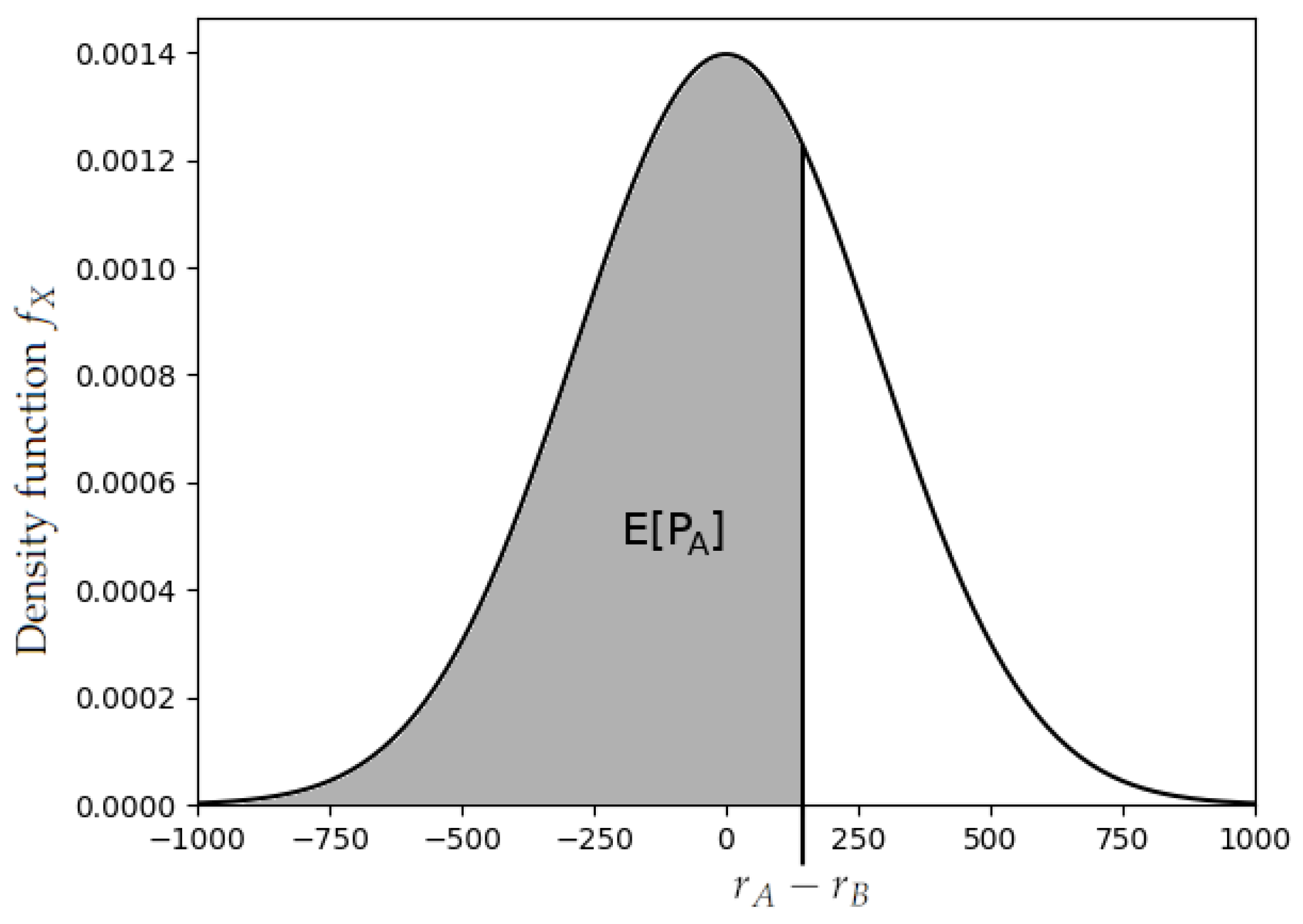
Here, K is a positive constant, and is the distribution function of some random variable X with mean zero, as depicted in Figure 1. The distribution function of X must also be symmetrical around zero so that . X was originally a normal variable, but it was later changed to follow a logistic distribution in the FIDE’s ratings. This has been argued to produce better predictions [1] (Chapter 8.41), and it also leads to an explicit and more meaningful expression for . In fact, sometimes, the update rule is given simply as
for some .
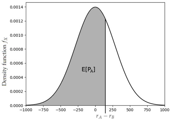
Figure 1.
Expected score versus rating difference.
It is also possible to update the ratings with the results of a set of matches (for instance the results of a tournament). Given a sample of matches with n intervening players , where the kth match is between players and and ends with scores for and for , and given initial ratings , we similarly compute:
Obviously, if a player outperforms their expected score, their rating increases, and otherwise it decreases, but the total sum of ratings does not change, as we will see later. However, before discussing the update rule, we need to review the model where the expected score originally comes from, which we refer to as the static Elo model.
2.2. Basis of the Static Elo Model
The difficulty in rating chess players versus, for instance, Olympic runners, is that in the latter sport there is a magnitude, the finish time, which does not depend on the rivals. For instance, taking a weighted mean of the latest times of each athlete would be enough to compare them, and objectively establish which are better and by how much.
However, Elo considers [1] (Chapter 8.23) what happens if we do not know the finish times and can only compare athletes by looking at who finishes first in head-to-head races. If the finish times of runners A and B follow distributions and and are independent, then
In general, if the times follow the same continuous distribution Y with different means, i.e., and , we can define and
which is exactly Equation (2) for (note that the lower the time, the better the athlete, and the higher the rating should be). Also, by definition, X has mean zero and follows a symmetrical distribution. Therefore, Elo’s system simply tries to estimate those underlying means from several match results and a given .
It also follows that , so the can only be determined up to the addition of a constant (we can only estimate their pairwise differences). Finally, , so scaling X does not affect the model either (it only scales the ratings). This means that both the average of the ratings and the variance of X are an arbitrary choice, and only the shape of affects the behavior of the model.
Traditionally, 1500 is chosen as the average rating [2] (p. 621) although Elo’s initial choice was 2000 as the average rating and as the standard deviation of X [1] (Chapter 8.21). This was replaced by the logistic distribution , which has a similar standard deviation of .
2.3. Statistical Inference in the Static Model
For the model presented above, the next logical step is to estimate the ratings of the players given a sample of matches (for instance a tournament). Again, we denote the sample by with , and if player i play match k, we use as shorthand if and if . We also denote the indices of games played by j with . Then, an interesting estimator is the one that reduces to zero the errors defined by
As we see later, this estimator is related with the adjustment formula in Equation (4), and in particular, if it exists, it is a fixed point when adjusting with that same sample M:
In fact, given a sample with n players, there are errors to minimize (since they add up to zero) and ratings to adjust (since the sum does not matter), so we should expect the estimator with zero error to be unique, and thus the only fixed point of the adjustment formula. In Appendix A, we characterize its existence and prove uniqueness in the case that it exists. Convergence is easy to see for the case of two players i and j, because if the results of a game follow Elo’s model, i.e., Equation (2), and are the estimators produced by the sample of the first m games, then by the law of large numbers
and since is continuous and has an inverse, converges to . Note that if the average estimated rating is the same at every step m, then for every j. Therefore, when we look for numerical methods to compute it, it makes sense to keep the average constant, and only worry about the convergence of the pairwise differences.
Finally, there is another natural way to estimate the ratings for a sample, if X is a logistic variable and there are only two results in the game (). In that case, the sample can be encoded as a set of independent variables where if , if , and otherwise (if ), . The static model then gives
which is precisely the formula of the logistic regression of against X. Since only depends on the variance of the distribution, and the choice of variance does not affect the model, we can just estimate by performing a logistic regression on the .
2.4. Basis of the Elo Adjustment Formula
So far, we have worked assuming Equation (2) holds and each player has a constant “true” rating . However, in practice, the strength of chess players or soccer teams changes over time, and hence the need for a system that updates the ratings with each new game and not with the whole history.
This is the reasoning behind the update formula in Equation (1): if we consider only one match between A and B, with estimated ratings and real ratings (and for simplicity, we pick ), then using Taylor’s expansion, such that
Therefore, for a small enough K, in particular for , this gives
and thus, if is fixed, converges to as is updated over an increasing number of games. In practice, K is chosen much smaller than —for instance, the FIDE uses for players with ratings above 2400, and in that case, , so a better K for accelerating the convergence of the expectancy would be .
The reason for the difference is that faster convergence is at the expense of a much higher variance of (the variance is proportional to ). If we apply the update formula over an infinite number of games, even if the true ratings of the model stay constant, the computed ratings do not converge, and they approach a limiting distribution [11], the variance of which we would like to minimize.
Therefore, the choice of K depends on the dynamic properties of the strength of the players. If we expect this strength to change significantly from one game to the next, K should be bigger, and if we expect the skill of the players to be relatively stable (for instance, if many games are played in a small lapse of time), we choose a lower K. The FIDE uses for younger players, who may improve quickly, and as said above, for players with rating above 2400, which are usually grandmasters and do not improve their play that fast.
2.5. Asymmetric Games
Until now, we have assumed that for two players of equal strength, each has an expected score of , but in practice, this is not true: in chess, for instance, the player with white pieces makes the first move and has a slight advantage. In the team sports we consider later, it is well known that if a team plays on the home field, it also has an advantage over its rival. To incorporate this in the Elo rating system, when A has a systemic advantage against B, we can use the following expectancy formula [3] (p. 36):
Here, L is a positive constant, which should obviously be bigger for a bigger advantage of A, since is increasing in L, and reduces to our symmetric model. We can estimate it given a sample of matches, provided of course that we know which player has the systematic advantage in each match. From now on, we suppose that in the kth match of a sample M, has the advantage. In particular, if X is logistic, L can be estimated as the independent term in the regression formula in Equation (10).
2.6. Accuracy Metrics for Elo Rating Systems
In order to determine the predictive accuracy of a rating system, we use several tools. The first one, provided by Arpad Elo [1] (Chapter 2.6), is a statistical test of normality for a sample in which the players have preexisting ratings R and each player plays m games. Originally the sample was a chess tournament, or a set of tournaments with the same m [1] (Chapter 2.7).
Elo proposes to represent the values of the residues in a histogram and to compare them with the frequencies of a normal variable with mean zero and the sample variance. Since is the sum of m variables, if m is high enough and the rating differences are not too high, by the CLT, each should approximately follow a normal distribution, with variance . More sophisticated normality tests, like the normal probability plot, can be carried out for the same variables.
In order to compare the accuracy of different systems in the same sample, we propose looking at the average of the squared residues across all matches, i.e., the mean squared error of p:
We can decompose this sum using the known expression of the mean square error, which is the square of the bias plus the mean variance:
In particular, when applied to the results of the games, we obtain:
The advantage of this measure is that we do not require any of the assumptions of a normality test. The sample can be extended in time (we can update the ratings between games using Equation (1)), and we do not need every player to play the same number of games. Also, if we apply two different rating systems to the same number of games, we can look at the variance reduction and extrapolate p-values to determine if one system is better than another.
However, unlike in a linear regression model, the results do not have a constant variance, so the expression (mean result variance) can only be understood as the expected variance of a game, i.e., , dependent on some distribution of the rating differences . We can only compare results from different samples if we assume this average variance to be similar, but this is not the case in general (for instance, decreases as the dispersion of the ratings increases).
If we assume the results are binary (), we can use other approaches. For instance, if is logistic, as we saw in Equation (10), the model is equivalent to that of a logistic regression. This allows us to compute statistics like the deviance D, which is approximately distributed as a chi-squared variable for large samples, by Wilks’ theorem [12]:
where, as before, n is the number of players.
Finally, the effectiveness of the model can be gauged more visually by plotting the receiver operating characteristic (ROC) curve. Again, this does not work with other possible results besides a win or a loss, such as a draw (), unless the non-decisive results are removed or imputed (for instance, to zero and one with probabilities and ).
3. Stochastic Elo Models
In many competitive team sports, we do not just observe the result of the game, but also a stochastic process , which determines the result at time T (we assume T is a positive constant, although it could be any stopping time of ). In practice, represents the score difference at time t, positive when the home team is winning, so the home team wins when , while the visiting team wins when .
Our goal is to extend the Elo model to incorporate , so that the expected result of the game at time matches the static model. In other words, we want to obtain an expression for such that , i.e., our initial guess matches that of the original Elo model.
We studied several possible models, but there are some properties they all verified. First, since (in the sports we chose) the past states of the scoreboard are not relevant to the game, and only the final score determines the result, should have the Markov property. As a consequence, both and should be martingales, by the Tower Property () [13] (p. 46).
Furthermore, for , since gives us as much information as and together, our estimation at time s should be better than the one at time t, and therefore
3.1. Continuous Models
Recall that in the original Elo model, team A wins if , and that should match the odds of being positive, so we can assume is times some constant. Since the incentives of the teams are the same at every point of the game (score the most points and have the opponent score the least), we can also assume the increments are independent (for disjoint intervals) and identically distributed.
For this to make sense, must be infinitely divisible. Although the logistic distribution is infinitely divisible [14], the increments are not logistic, so we suppose that X and are normal, and in that case, the increments must also follow the normal distribution by Cramér’s decomposition theorem [15], so has i.i.d. Gaussian increments, and it is a Brownian motion with drift:
where is the standard Brownian motion, i.e., , and B has independent and normal increments . Under this model, used by Stern in [4], if we want this expectation to match the one given by the static model, we must have
and from this, we immediately obtain the expected score conditioned on :
Similarly, if we condition on an arbitrary score difference at time , we obtain
Denoting by the fraction of the time that remains, and by C the constant coefficient , we have:
In the end, we obtain an expression where the term depends on the ratings and decreases to zero as the time t approaches T, while the term depends on the score and becomes larger as the game nears its end, as we would want (unless ). In other words, the behavior or as is exactly what we would expect.
Note that setting , and assuming a game starts with a score difference of S points, the expected score is . This allows us to interpret the constant C as the handicap (measured in rating points) that each goal or point entails at the start of the game. We could in fact use this to estimate C from game data, although we do not need to pick . For any , C should minimize the mean square error
as long as the model is correct, and the minimum should be the same for every t. Conversely, if the function above is minimized for for every t, our model is optimal among a certain class, as the following result showcases.
Lemma 1.
If there are functions and , and there exists a such that for every , then for every ,
Proof.
□
In particular, for and the function , this means that our model is optimal among the ones with a prediction of the form . If we further suppose that the true expectancy has the form , we can estimate f by looking at the times in the sample where , and if minimizes the mean square error over that restricted sample, our model is optimal among this wider class.
Finally, assuming we already know or have estimated , we can obtain the drift and express in terms of known quantities as
Finally, notice also that , which gives another way to estimate C.
3.2. Accuracy Metrics for the Stochastic Model
If we take in Equation (26), we obtain
Therefore, the residuals follow the same law as X (the variable used for the static model), and we can do a normality test on them, for instance through a QQ plot or comparing a histogram with the predicted frequencies for X. We could in principle use Equation (23) with any distribution of X, and in that case, minus the rating difference follows the law of X, and the same test works.
From Equation (26), we can also reconstruct the standard Brownian motion in the model:
and since is a standard Brownian motion if and only if is, taking , we obtain that is a standard Brownian motion in as a function of , which is just the fraction of the game time elapsed at t.
From Equation (26), we can also deduce
That is, if we compute the mean squared error of instead of at each time t, we should obtain a linear function in t, and we can test this hypothesis via linear regression.
Recall that we are assuming the increments of are independent and identically distributed, and in particular, the variance of only depends on t. We can test this directly by looking at the points scored by either team at each interval between 0 and T, or, if can increase or decrease by amounts other than one, we can see if the sample variance depends on t.
Finally, this continuous model implies expressions for and for each t, and we can check if they behave like martingales in a sample of games.
3.3. Non-Homogeneous Process
In practice, does not always behave like a homogeneous process in time, that is, more points may be scored in some sub-intervals of than others. In that case, if for some increasing function m, we can model the process as
where behaves like the score in the first model. Since this is a map of the process that we were using before, we can use the homogeneous model to compute
which is exactly the same as before, for .
3.4. A Discrete Model
The main difference between this model and the actual score difference is that the former is a continuous process, but the latter is discrete in value () and continuous in time. The process that fulfills this condition best is a Skellam process, as described in [6], i.e., the difference of two Poisson processes with different rates, which model the score of each team or player during the game.
If and are two independent Poisson distributions with mean and , then their difference is said to follow a Skellam distribution, . If and are independent Poisson processes with rates and , the process
has i.i.d. increments as well.
However, in this case, modeling the score with is not so straightforward. For starters, if we multiply by a constant, we do not obtain another Skellam process. Adding a real-valued function of t also changes the domain of the process from to . Therefore, the only option is to assume that
This in turn means that we cannot assume homoscedasticity of the process, because a Skellam distribution with parameters and has mean and variance . Since and are non-negative, the mean is less or equal to the variance, and if we fix , we would put a bound on the expected final score , which is not realistic.
However, the distribution of , which should have the same shape as X, now depends on two parameters, and not just on the rating difference . We can remove this degree of freedom by fixing a relation between and , and for simplicity’s sake, since the probability that takes the value k is
we can fix to compute only once for each . Here, is the modified Bessel function of the first kind [16], which does not have a closed-form expression.
To determine how and depend on the ratings, we can take to be linear in the rating gap as in Equation (26), and then, if we pick so that , from the product and difference of and , we obtain a second-degree equation
from which we finally obtain not just a prediction for , but also a probability for each possible final score, and in this case, the probability that is positive, so we can include draws in our model. In particular, if we assign a result of for draws,
Similarly, if we consider that expression as a function of , it can be shown that it is increasing (see Appendix B), and with limits 0 and 1 at and ∞. Therefore, for some random variable X, and then this model is also an extension of a static Elo model.
4. Computational Study
Next, we evaluated the performance of the proposed stochastic extensions of the Elo system in a computational study implemented in Python. All the results discussed can be replicated with the code available at https://github.com/gonzalogomezabejon/StochasticElo (accessed on 19 July 2024) using real data from reference databases for each sport (see Data Availability Statement), which are also included for download through the previous link. In the case of soccer, a comparison with the more complex methodology of the Soccer Power Index (SPI) developed by Nate Silver [7] was also carried out.
4.1. Experimental Setup
In order to evaluate a rating model with any of the accuracy metrics exposed in Section 2.6, a sample of matches M for which both players have a rating is needed. Furthermore, the update formula in Equation (1) needs preexisting ratings, so we used some of the games in our dataset to estimate the starting ratings of each team, using the estimator defined in Section 2.3.
On the other hand, the proposed stochastic models were designed for sports or games where the result depends on a numerical score (S) and the match has a fixed duration (T), such as soccer, basketball, or ice hockey, although we omitted the latter in the experimental results for brevity. Moreover, we focused on league competitions, where each team plays more games and we could use a bigger sample to obtain . For instance, in the Premier League, 20 teams play 380 matches, while in the World Cup, 32 teams play 64 matches.
Most national leagues have a similar format, consisting in yearly seasons in which most of the participating teams remain the same from one year to the next, and all teams play the same number of games each week. We designed an algorithm to extract rated games from any of these sports as follows:
- The expected result was determined by Equation (13) with constant L.
- During each season, we denoted by “entering teams” the teams that did not play the previous season (during the first season, they are all entering teams).
- We divided each season in two parts (I and II), the former comprised of the games that started before every entering team had played at least m games.
- During part I, in each match between two non-entering teams, we updated their ratings (from the previous season) according to Equation (1) using a fixed factor K.
- When part I ended, we computed the rating estimator for each entering team using the games in part I and the current ratings of non-entering teams.
- During part II, since we had ratings for all teams, we could just update them every match using Equation (1) with the same K factor.
In this way, we had a rating before the start of the game for the matches between non-entering teams in part I of each season, and all matches in part II, and we could use them to evaluate the rating system.
This algorithm has (hyper-)parameters m, K and L, that is, the length of part I of each season, the sensitivity of the Elo system to new results, and the home field advantage, respectively. We fixed m and estimated K and L by minimizing the mean squared error defined in Equation (14).
4.2. Basketball Results
Basketball has several advantages regarding the Elo system. First, it only admits two results (win or loss), so the result follows a Bernoulli distribution and the logistical model in Equation (10) can be used. In addition, the score variable has a relatively large range (each team scores around 100 points) and changes quickly (by 1, 2, or 3 points each time), so we do not lose too much by approximating it by a continuous variable.
On the other hand, an NBA basketball match lasts 48 min divided in four 12 min quarters, but if the scoreboard is even at the end of that time, additional 5 min quarters are played until one team is ahead. We ignored these extra quarters for the sake of simplicity, since we assumed T was fixed, and our prediction at the end of the game would be slightly wrong when .
Our dataset for basketball consisted of the NBA league games between the seasons 2000–2001 and 2023–2024, obtained from www.basketball-reference.com (accessed on 19 July 2024), which registers every change in the score and its time (in seconds).
4.2.1. Static Elo
We implemented the algorithm described above for and , corresponding to a normal variable , in a training set of seasons 2000–2001 to 2009–2010, and in four different ways to test the effectiveness of the Elo model and the significance of its parameters:
- Without Elo, simply assuming .
- Fixing and minimizing as a function of L (no change in strength).
- Fixing and minimizing as a function of K (no home advantage).
- Minimizing as a function of K and L (standard Elo system).
To avoid overfitting in K and L, we also implemented the algorithm for the optimal values and in a validation set consisting of seasons 2010–2011 to 2023–2024. The mean squared errors in the training and testing sets are summarized in Table 1:

Table 1.
Mean squared error of different Elo models vs. sample variance.
We can see straightaway that the Elo explains a significant part of the variance (around 11%), and both parameters are useful, since setting them to zero increased the mean squared error. The reduction was similar in the training and testing sets, so cross-validation shows the robustness of the algorithm in Section 4.1.
Notice also that the K-factor and home field advantage are similar to those of chess, where [1] (Chapter 8.93). The sign of only reflects that in basketball (and American sports in general) the visiting team is listed first.
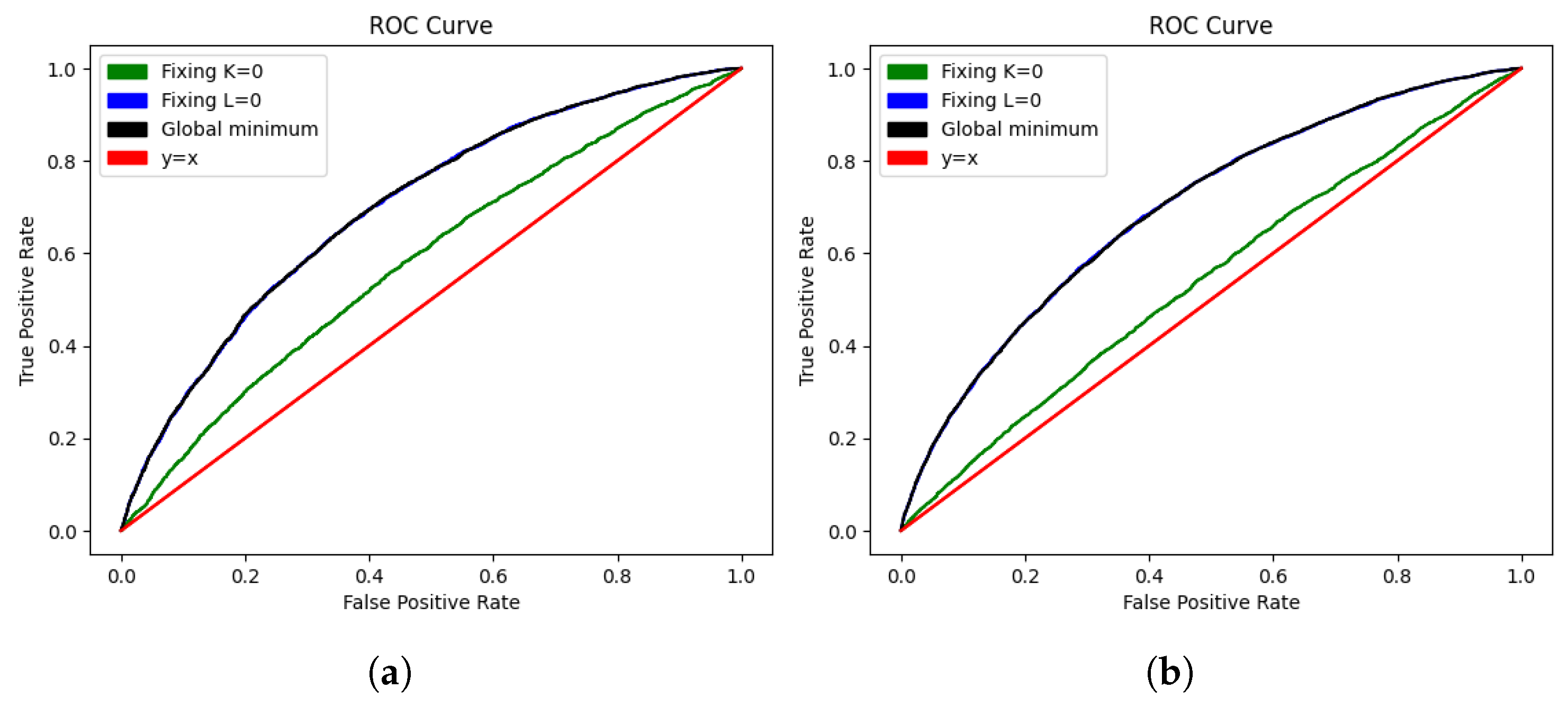
We note that setting (which amounts to leaving the rating of a team unchanged until they are relegated) increased the variance, but it still had predictive power, as evidenced by the ROC curves shown in Figure 2.
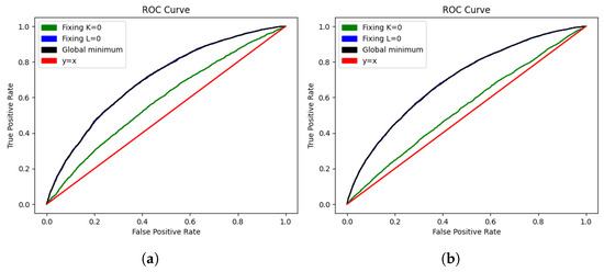
Figure 2.
ROC curve for each of the Elo system implementations in the training set (a) and test set (b).
Finally, setting barely changed the curve, because the map from to is a monotone increasing bijection, and the order of the expected result under the two models are the same for equal (and indeed the K factors were very similar).
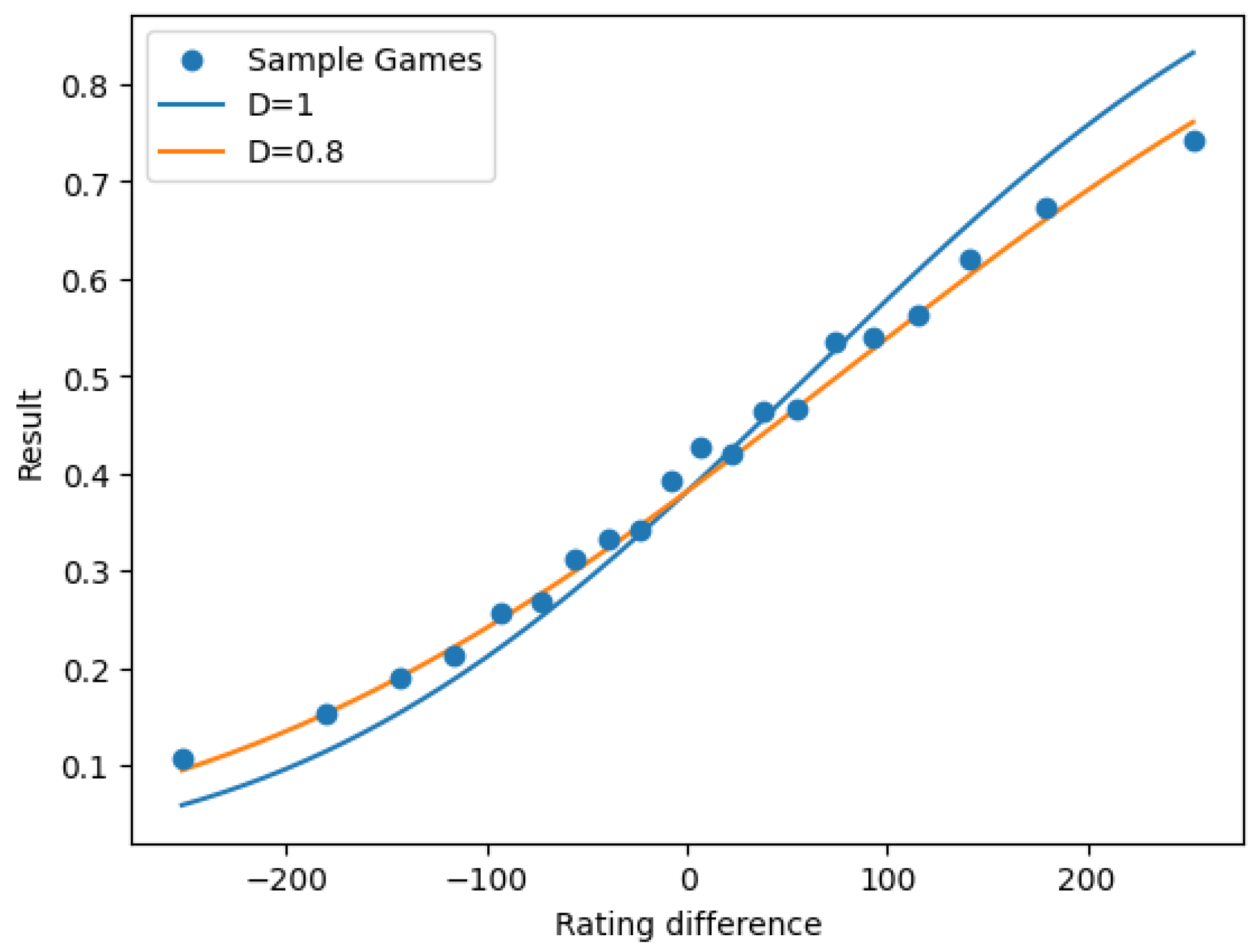
After fitting our model and obtaining the sample, we could expect that for a subsample of matches with rating difference , the average result would be close to , but this was not the case, as evidenced by Figure 3.
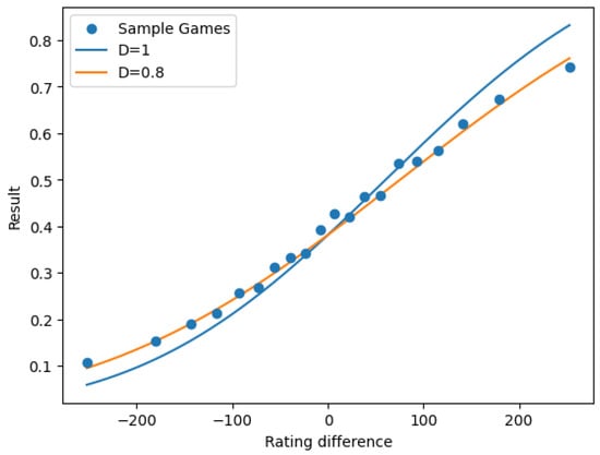
Figure 3.
Observed expectation of vs. versus predicted value .
We observe that the normal distribution function overestimates the effect of the rating difference in the expected result of a match. We can obtain a better predictor if we multiply by a “dampening” constant , as in Figure 3 of [17].
When we minimized the on , and D (only using D for the calculation of the mean squared error, since otherwise we would just be scaling X), we obtained optimal parameters , and , reducing the to 0.21064 in the test set.
This seemed a small improvement in , but we could test the significance of the reduction in variance by looking at the variables and for a random game.
In order to check if had a positive mean from our sample of games, we sampled the difference and argued that by the central limit theorem, the sample mean of Z approximately followed a normal distribution with n times the sample variance of Z. In our testing data, Z had a negative mean with , so D significantly improved our predictions.
4.2.2. Stochastic Elo
Our algorithm left us with 12,500 rated games out of the 12,933 games in the training set, and 17,437 out of the 17,820 originally in the testing set. These 17,437 matches were the ones used for the analysis of our stochastic model.
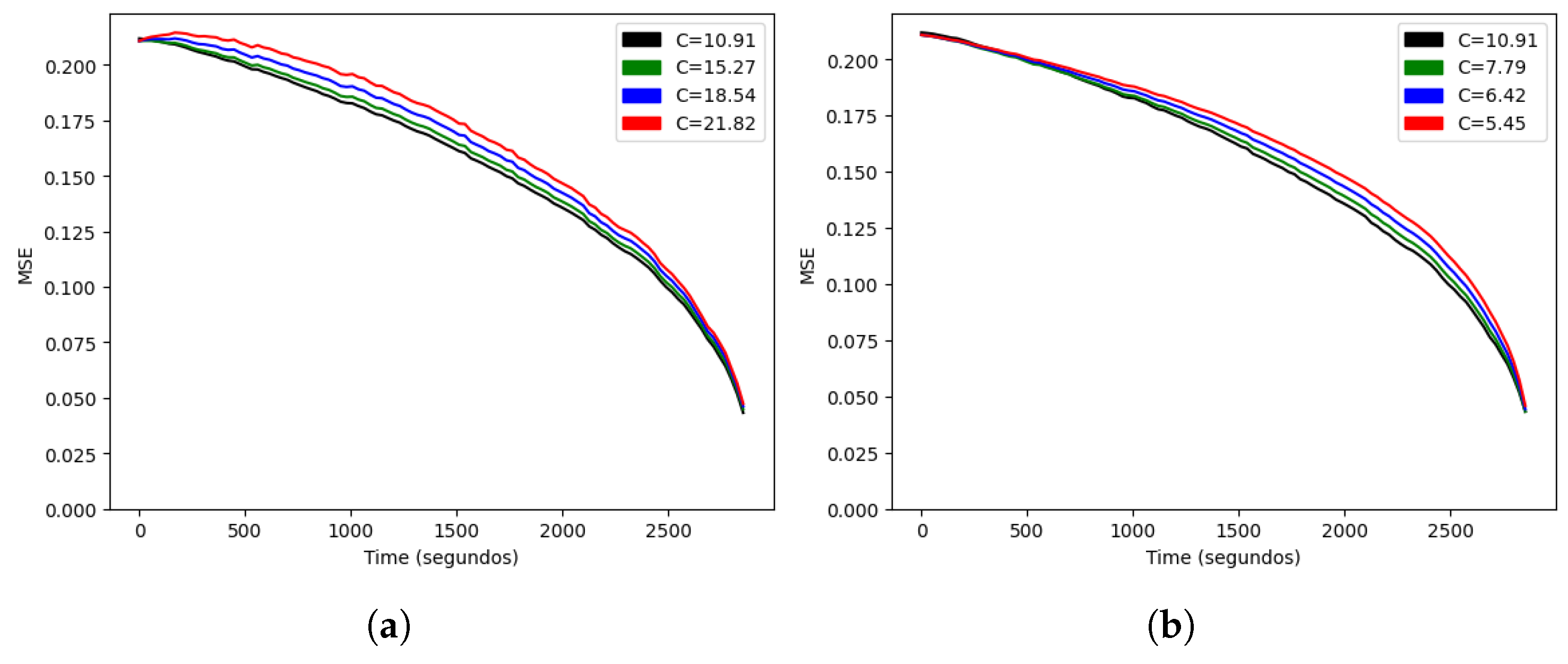
We started by estimating the only parameter of the stochastic model, C. As we showed in Lemma 1, if the model is correct, the optimal value should minimize the error at every time t, so we minimized the average of that function at different times for a more robust estimation of . In the training set, we obtained , and we could compare the function for higher and lower values, as shown in Figure 4. Since every curve lay above the curve for , Lemma 1 suggested that our formula for the expected result was optimal among the family . We also noted that the error did not reach zero at the final time of 2880 s, since a tied score at that time results in an extra time being played. Our model assumed a fixed duration, so in order to predict the result beyond minute 48, we would need to model another (shorter) match.
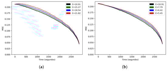
Figure 4.
Mean squared error as a function of time for (a) and (b).
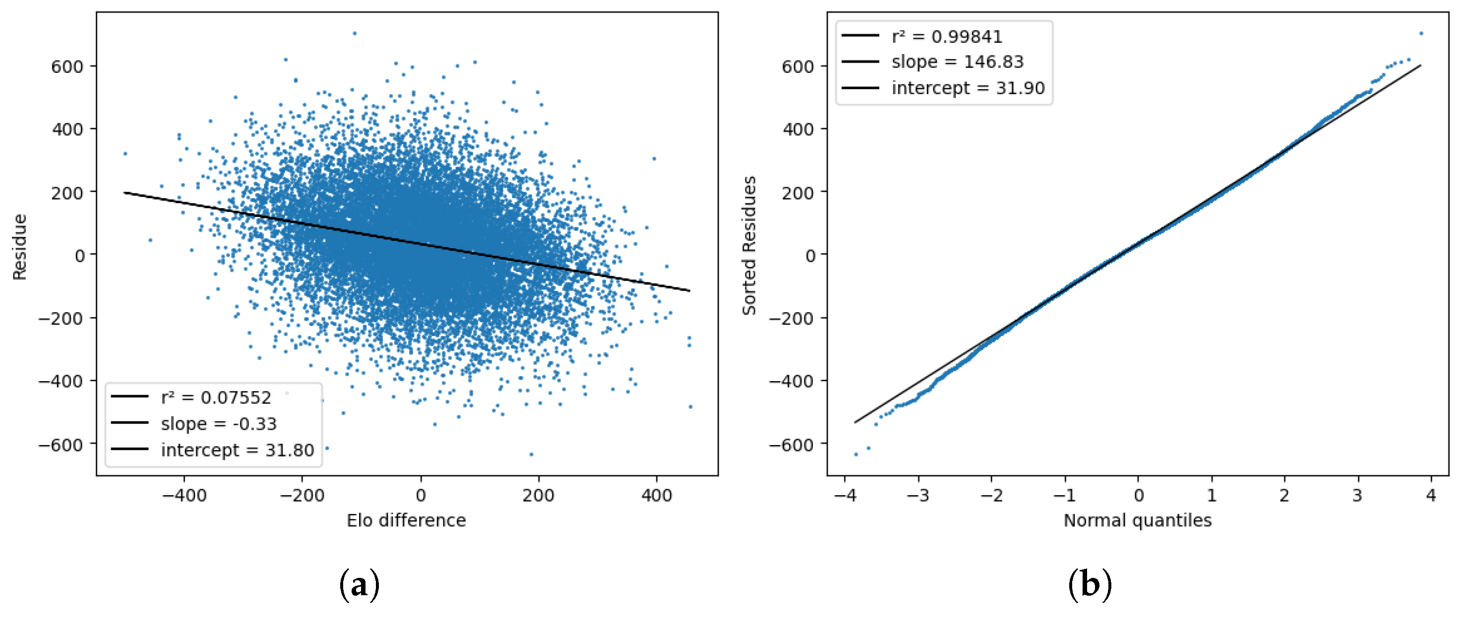
Next, Figure 5 shows the result of checking the normality of the score process by computing the normal residues and comparing them with the quantiles of a normal distribution. Here, again, is the score after the first 48 min, not the final score of the game. As expected from Equation (27), the residuals more or less followed a normal distribution, but the mean was not zero, meaning the home team scored better (in terms of ) than the Elo model predicted. The standard deviation was also smaller than the expected value of the model, namely, . From the first plot, we can also tell that the residuals were somewhat correlated to the Elo difference but not to an extent that would invalidate the model.
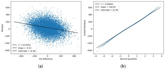
Figure 5.
Tests for the model residues , plotted against the Elo difference (a) and the standard normal quantiles (b).
In this type of figures, the black line is just a linear regression fit to the actual data, which correspond to the blue dots. Finally, Figure 6 checks the linear relationship between the score variance and time, as described in Equation (29), by computing the quantities
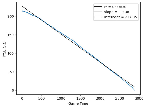
Figure 6.
Score prediction variance vs. match time.
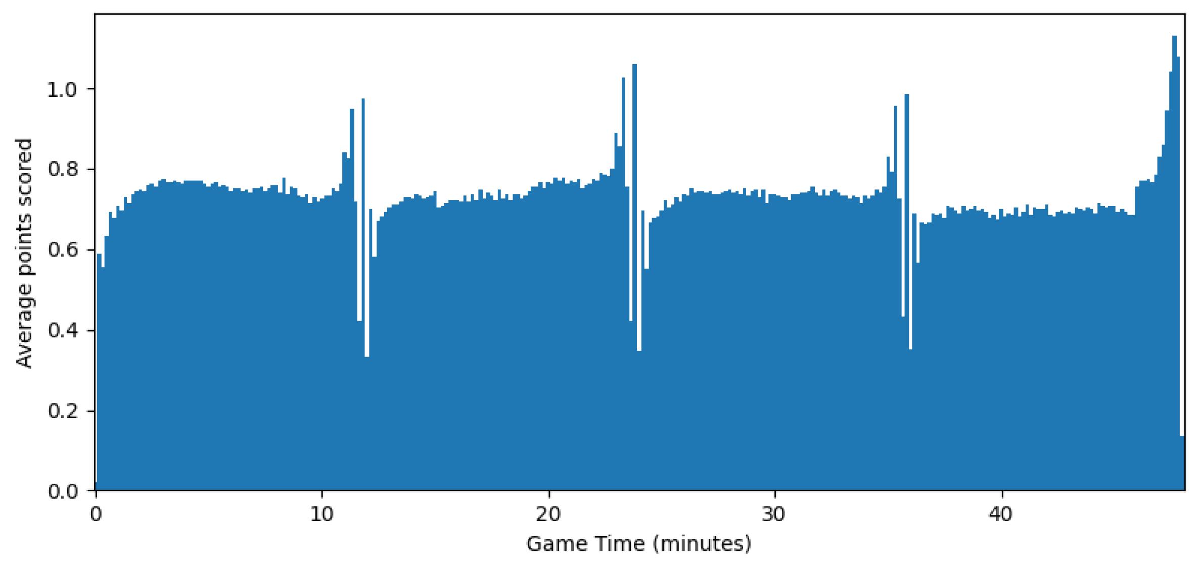
The resulting function was close to a line, but the variance still dropped more quickly at the end of the match than at the beginning, suggesting was not completely homogeneous in time. Figure 7 plots the average number of points scored at each 10-s interval of the game by either team, in order to approximate the variance of that interval (they are in fact equal if we assume the score is the difference of two independent Poisson processes as in the discrete model). However, Figure 7 shows that the process was very homogeneous in time, except for brief periods before the end of each quarter.
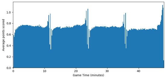
Figure 7.
Average increase in combined score vs. match time.
4.3. Soccer Results
Soccer was somewhat more challenging than basketball when it came to applying Elo models. First, since our database consisted of league games, we did not have extra times, at the expense of allowing for draws () if the score was tied at the end of the match. We should note that in both the Premier League and the Spanish First Division, teams are awarded three points for a victory, one for a tie and zero for each loss, so this is not entirely a zero-sum game, whereas in the Elo model, .
Although there are no extra times, there is time added at the end of each half-time, but our database only kept track of the minute in which each goal was scored, and every goal scored in the added time appeared at the minute 90 or 45. Finally, was relatively small (usually ), so approximating it by a continuous variable was problematic.
Our dataset for soccer consisted of the seasons 2003–2004 to 2023–2024 of the Spanish and English first division leagues, both counting 5320 games. We used the former for training and the latter for testing. The data were obtained from https://fbref.com/en/ (accessed on 19 July 2024).
4.3.1. Static Elo
Since the league structure was similar to that of the NBA, we used the same algorithm in Section 4.1 to obtain rated games, this time with a sample of for part I and the same , now also adding the dampened model to the table along with the optimal D. The corresponding results are presented in Table 2.
Table 2.
Mean squared error of different Elo models vs. sample variance.
As we saw for basketball, both K and L were clearly significant, but the reduction in variance for adding D was much smaller. Using the statistical test described for basketball, we see that D is significant with , and the optimum was closer to one.
4.3.2. Stochastic Elo
After implementing the static Elo system, we were left with 7176 matches out of the 7980 in our testing set, and we used these for the analysis of the stochastic model.
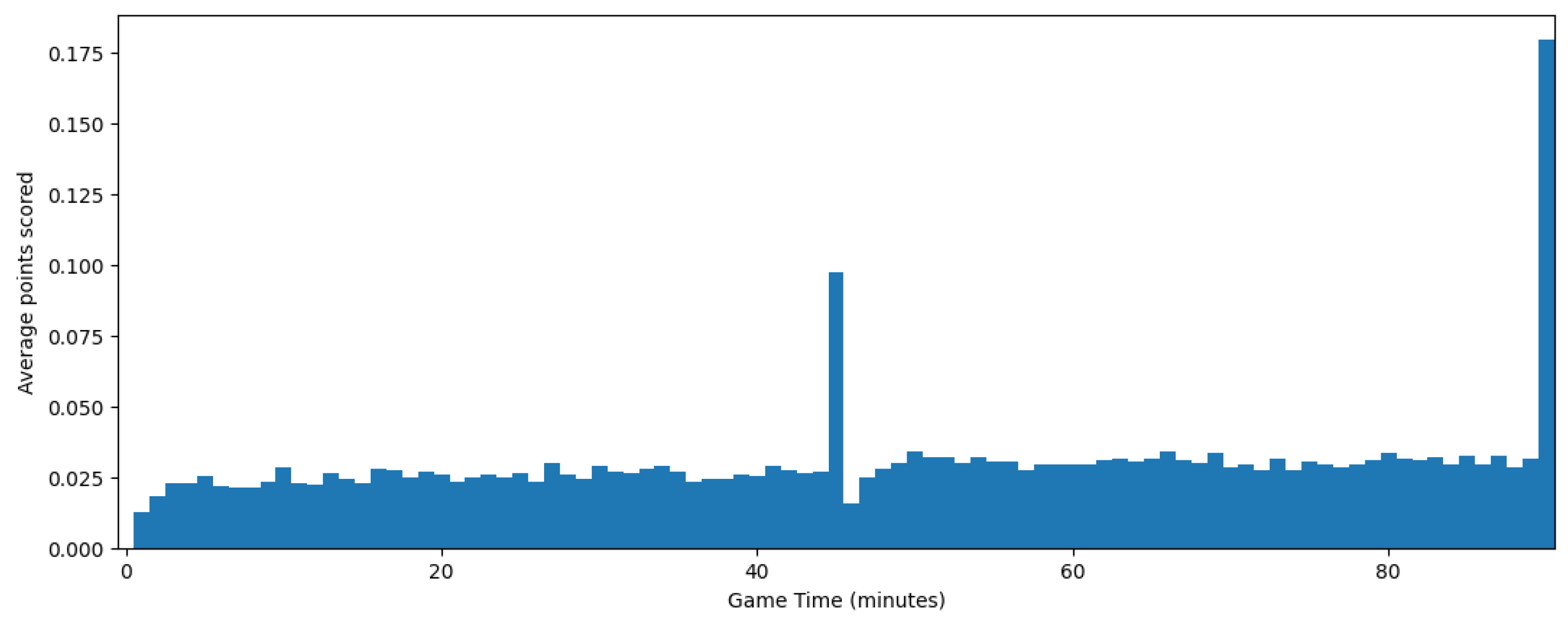
However, in this case, the irregularity of the process versus the recorded time was stronger. As shown in Figure 8, the number of goals scored by every team each minute increased as the game neared its end and had two spikes in the added time of each half, which makes the simple model we used for basketball less effective.
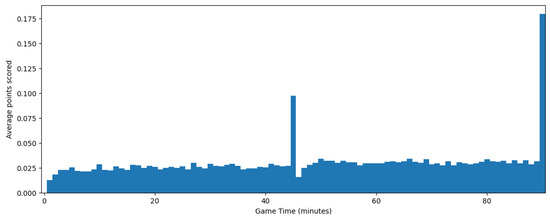
Figure 8.
Average number of goals each minute.
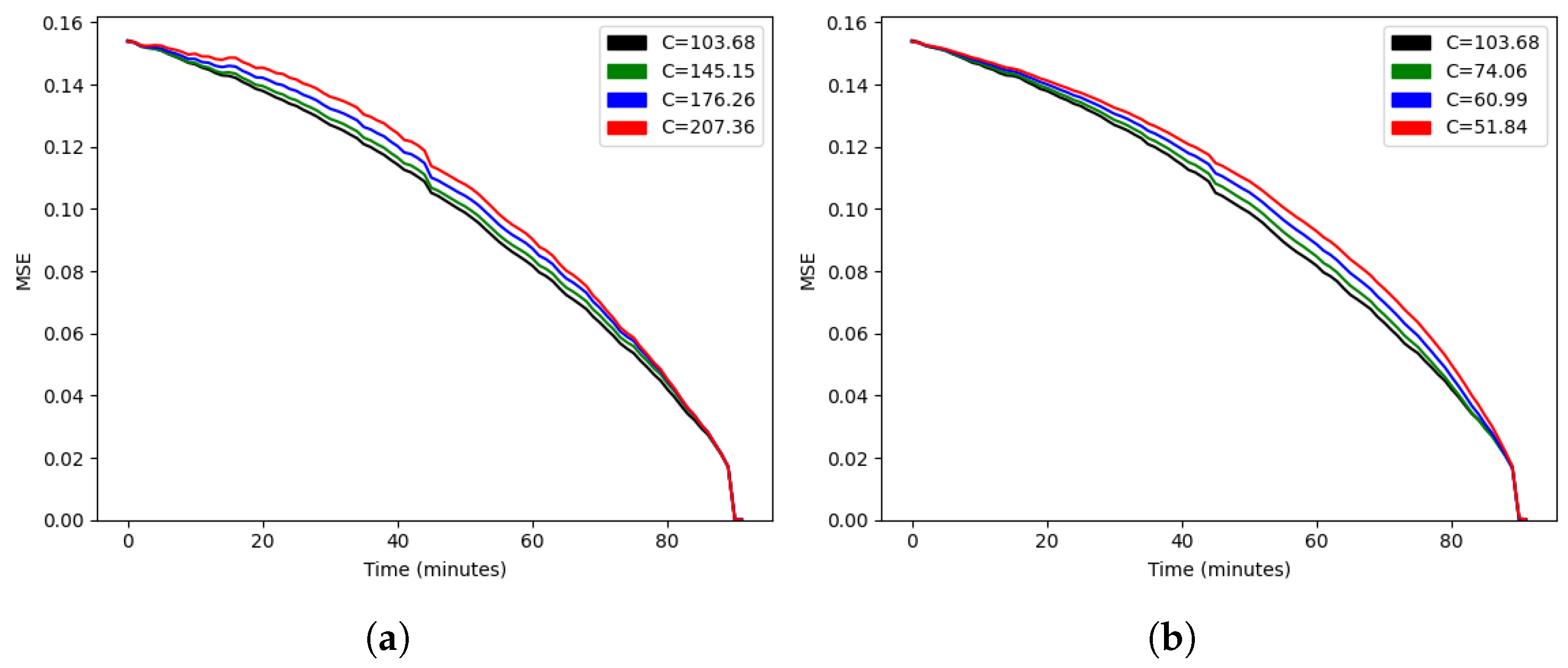
If we estimate C by minimizing the average of at evenly spaced points t, with linear , we obtain the functions and depicted in Figure 9 and Figure 10, respectively.
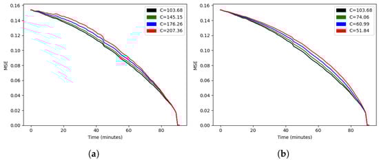
Figure 9.
Mean squared error as a function of time for (a) and (b).
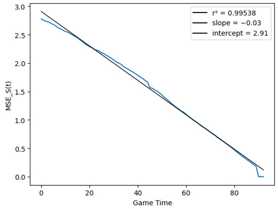
Figure 10.
Score prediction variance vs. match time.
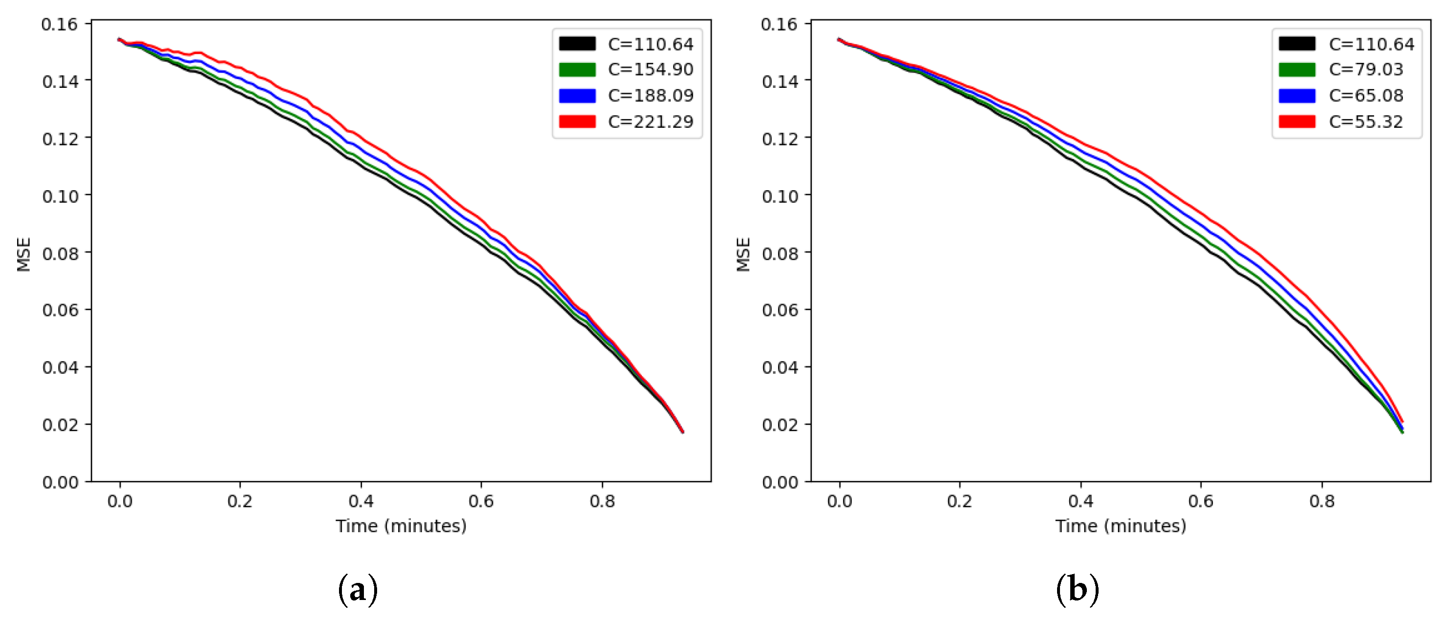
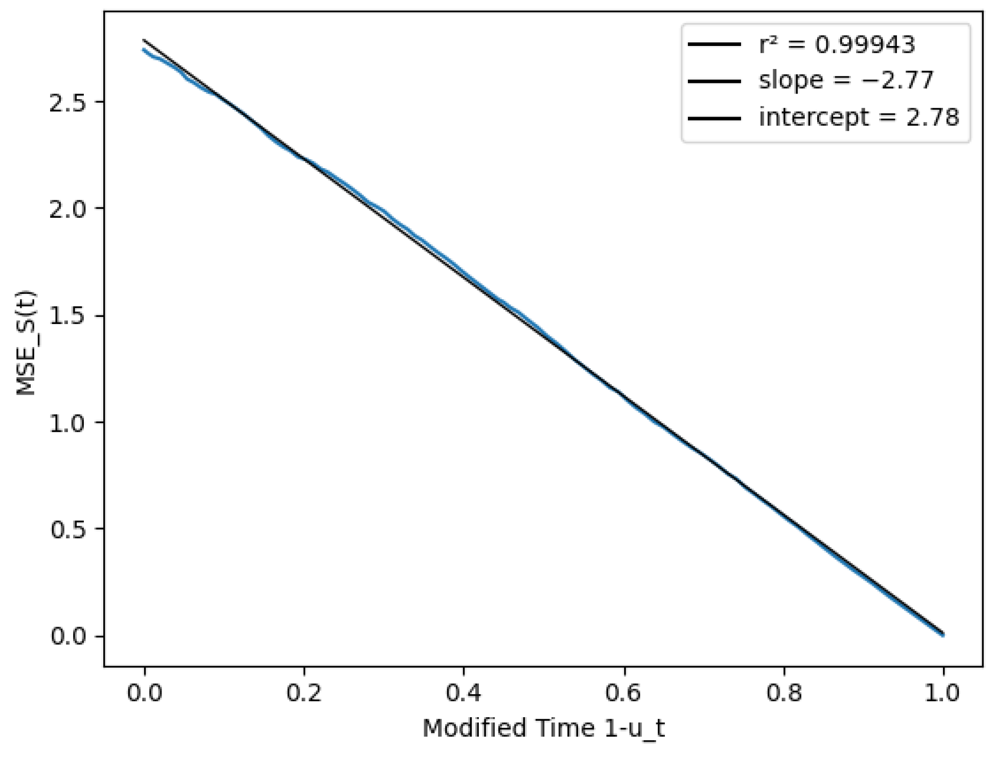
To tackle this problem, we modeled the process as a non-homogeneous process, with equal to the fraction of goals in our sample scored after time t. To show the results with this modification, Figure 11 and Figure 12 replace the match time on the x axis with the modified time . The last plot showcases that the score variance (conditioned on ) was almost exactly proportional to , and that our assumptions on the process were reasonable.
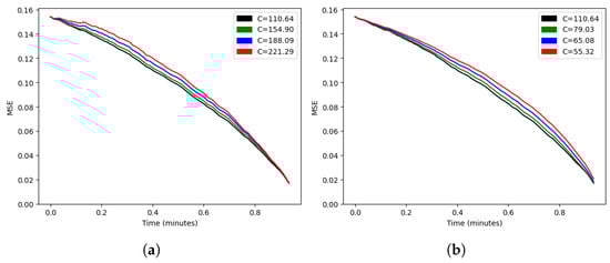
Figure 11.
Mean squared error as a function of for (a) and (b).
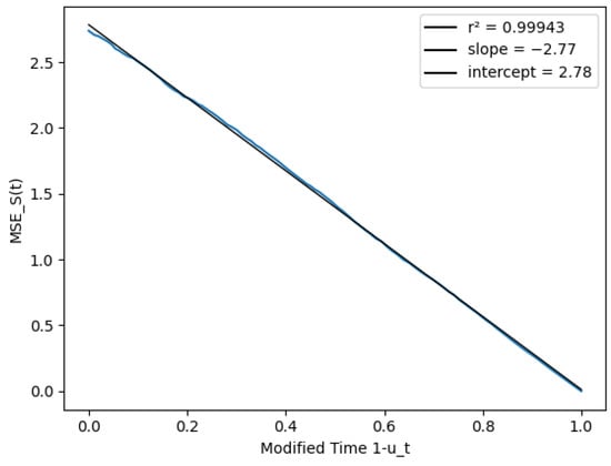
Figure 12.
Score prediction variance vs. modified time .
Finally, Figure 13 plots the residues and compares them to the standard normal quantiles and their respective rating differences . The distribution of the residues was close to normal, except for slightly thicker tails. The correlation between the residues and the rating differences was virtually zero compared with the one we saw for basketball.
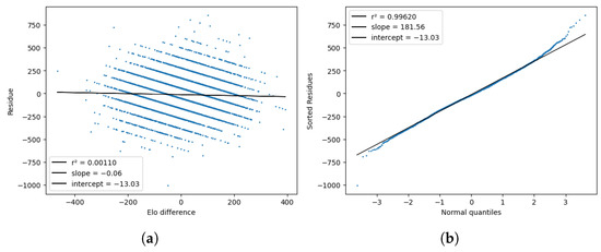
Figure 13.
Tests for the model residues , plotted against the Elo difference (a) and the standard normal quantiles (b).
4.3.3. Discrete Elo Model
Lastly, we implemented the discrete score model based on the Skellam process. As we showed, this is a particular case of an Elo model, and thus the same algorithm can be used to estimate the parameters , and D. In this case, we used and the function defined in Equation (37). To estimate the only non-Elo parameter of the model,
we used the sample mean of the product of the goals in our training sample, obtaining . The corresponding results are presented in Table 3.
Table 3.
Mean squared error of restricted Elo models vs. sample variance.
Despite the distribution function being different, the mean squared error was very close to that of the standard Elo model with normal . However, this model also predicted probabilities for the three possible results, allowing us to compute metrics like log-loss [18].
For comparison, we implemented the rating system used by the Soccer Power Index (SPI) developed by Nate Silver [7], which uses two rating parameters for each team: one for their offense (their capacity to score goals) and another for their defense. A concise but complete explanation of the SPI system is given in Appendix C.
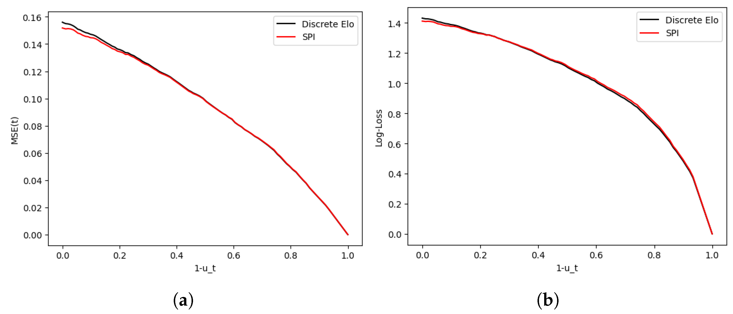
The SPI system achieved an of 0.1518 versus 0.1533 for the discrete Elo system, and the squared errors were significantly lower, with a p-value of . The average log-loss at time zero was also better, with 1.411 beating 1.432 for the discrete Elo and a p-value of . However, both systems also gave probabilities for the result being a victory, loss, or draw at any time t during the game, namely,
where and are the expected goals by the home team (A) and the visiting team, respectively. Computing these for every time t, we obtained the results shown in Figure 14.
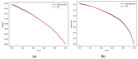
Figure 14.
Evolution of model mean squared error (a) and Log-loss (b) vs. modified time .
Note that in the log-loss curve, the Elo system beat SPI in the second half—for instance, at min, the log-losses were vs. with a p-value of showing that the Elo loss achieved a smaller loss. This suggests that despite being a one-parameter model and its relative simplicity, the discrete Elo system is on par with SPI in terms of predictive power when it comes to mid-game predictions (conditioned on ).
5. Conclusions
In this work, it was shown how the model underlying the Elo system had a natural extension for fixed-duration sports with which it was possible to model the score of each team. The proposed stochastic Elo system can be easily implemented for league competitions using the algorithm in Section 4.1, which in turn uses the estimator defined in Section 2.3, and supported by the results proved in Appendix A.
A discrete model for soccer was also proposed, which was also an Elo system at time and inherited its robustness and simple update formula, but modeled the goal difference as a discrete process, thus providing probabilities for each possible outcome of a match. Moreover, we saw that this system had accuracy comparable with that of a biparametric rating system like SPI across the duration of a soccer game. This suggests that the simplicity of the original Elo system may favor it as an alternative to sport-specific models, and its use will continue to increase in this context.
Future Work
These results certainly apply to games or sports with a score board and fixed duration in time, but they could be replicated for other sports with different scoring systems, like table tennis, where the game ends when the first player obtains a score of 21, regardless of how long it takes. It is possible that an Elo system can be derived from these types of “race” processes as we did for our Skellam process.
The concept of predicting the result of a match mid-game could also be applied to chess, where there is no objective score but it is common to obtain an “evaluation” from the state of the board, using chess engines. Some chess websites store extremely large databases of computer-evaluated games in which a study of this kind could be performed.
Another question we did not consider when optimizing the parameters of the Elo system, such as K or L, is whether the distribution function can also be inferred from a large enough sample of games. Obviously, the space of distribution functions is not finite-dimensional, but a method for choosing has not been proposed, even among a finite-dimensional family of distributions.
Finally, there are games (such as checkers) for which there is a concept of perfect play, i.e., a strategy that guarantees a victory or a draw. We can easily see that an expected result above implies an upper bound in ratings from the original model, but the Elo system does not have an upper bound built in. However, some models derived from race processes not only produce odds for a win, draw, or loss but also have a maximum or minimum rating associated with perfect play.
For instance, given ratings , we consider Poisson processes and with rates and , and arrival times and . Suppose player 1 wins when , player 2 wins when , and they tie when , for fixed , . Then, the strength of a player decreases with r, but if , player 1 will never lose, and zero is a lower bound for ratings. To the best of our knowledge, these types of systems have not been studied computationally at all.
Author Contributions
Conceptualization, G.G.-A.; methodology, G.G.-A. and J.T.R.; software, G.G.-A.; validation, G.G.-A.; formal analysis, G.G.-A.; investigation, G.G.-A.; resources, G.G.-A.; data curation, G.G.-A.; writing—original draft preparation, G.G.-A.; writing—review and editing, J.T.R.; visualization, G.G.-A.; supervision, J.T.R.; project administration, J.T.R.; funding acquisition, J.T.R. All authors have read and agreed to the published version of the manuscript.
Funding
This research was funded by the Government of Spain grant number PID2021-122905NB-C21.
Data Availability Statement
The raw data of soccer and basketball games was obtained from https://www.sports-reference.com (accessed on 19 July 2024) according to the data use policy in https://www.sports-reference.com/data_use.html (accessed on 19 July 2024). The full computer code for our computational study, as well as the files containing the basketball and soccer data used, can be downloaded at https://github.com/gonzalogomezabejon/StochasticElo (accessed on 19 July 2024).
Conflicts of Interest
The authors declare no conflicts of interest.
Appendix A. Proofs Regarding the Static Rating Estimators
In this appendix, we characterize the existence of the rating estimators that give zero errors for a sample of matches M (assuming is continuous), and prove the uniqueness of (up to adding a constant). We also prove that the vector is a descent direction for the problem .
Recall that our sample is given by , where is the “home” player or team, is the “visiting” player, and is the score of player , that is, one if wins and zero if loses, or an intermediate value like if there is a draw. Conversely, the score of is .
We want to characterize the existence of the static estimator, that is, the set of ratings that verifies, for every player j,
where and , . For the expectancy, we use , where L is a non-negative constant ( is the standard symmetric case). Finally, we define a digraph where if and only if for some k, and . We want to show the following:
Theorem A1
(Existence). For any sample M with weakly connected (connected as an undirected graph), there exists an estimator with , if and only if is strongly connected (that is, for every pair of players , there is a directed -path).
Theorem A2
(Uniqueness). If there are two estimators and such that , then
Lemma A1.
Proof.
□
Lemma A2.
If the players are partitioned in two sets with , then
Proof.
We sort the games of M in the sets , where the set contains the indices of the matches where the first player is in the set P and the second in Q. Then, by Lemma A1,
but since only contains games between players in I, again, by Lemma A1,
and finally, since every game in has exactly one player in I,
and we use the same argument in to obtain
as we wanted (since ). □
Proof of Theorem A1.
(⇒) If the static estimator exists but is not strongly connected, then there are players i and j such that there are no -paths in . In that case, if we define as the set of players reachable from i in , and to be the set of players not reachable from I. By construction, in a game and , if , we would have an edge between and , which contradicts the definition of I and J, so .
Note that and , so the sets are not empty, and since is weakly connected, there must be a game between a player in J to another in I; let us assume w.l.o.g. that , and in that case, by Lemma A2,
since for any , and that is not possible.
(⇐) On the other hand, suppose is strongly connected. Then, we show that exists by proving a stronger proposition: if we fix , there are such that for every , we have . To do this, we show by induction in m that there exist continuous functions for such that for any and , and also, that every component of is non-decreasing in each of its arguments (that is, ). For brevity, we write instead of .
First, we note that since is weakly connected, is strictly decreasing in , but non-decreasing in any other rating for :
since one of the sums is non-empty and is strictly increasing. From the same expression, we can infer that
For the base case of induction, , we can show that the increasing function has a unique zero, because
(since is strongly connected, player n scores less than one in some match k) and similarly,
and f is obviously continuous ( is continuous), so just applying the intermediate value theorem allows us to define as the only zero of f. To see that is non-decreasing in every coordinate of its argument, we check that
and the last implication is a consequence of being strictly decreasing in .
To see that is continuous, we note that for any convergent sequence with , we have
and since is strictly monotone and continuous, and therefore bijective, .
Now, for the induction step: suppose exists and is non-decreasing in and with respect to every coordinate, and . For a fixed , we show that the continuous function , which inherits continuity from and , is strictly decreasing.
Suppose . Then, by our induction hypothesis . Let us define and , and note that since , and . Note that or , and in the latter case by definition of . Using that fact, and then Lemmas A1 and A2,
where . Therefore,
since at least one of the sums is non-empty ( is connected), and for any game between and .
We also check that approaches a positive number as x goes to infinity. Since is non-decreasing in x, its coordinates either have a limit as x goes to infinity, or they also go to infinity (by the monotone convergence theorem), and we can define
for which, again, and , and as before,
since is connected and therefore one of the sums is non-empty. An analogous argument shows that as , and thus, for any given , has a unique zero, which we denote by , with that, we can define .
Now, we can show that is non-decreasing, because if , then by the induction hypothesis, , and hence
which implies (by the fact that is strictly decreasing and continuous, i.e., bijective) that .
This in turn implies that is non-decreasing by composition of g and , and to conclude the induction, we only need to check that g is continuous. This is similar to the base case, using that for any convergent sequence with , we have
and invoking that is bijective again.
Our induction works for , and to complete the proof (for ), we consider . By definition of , we know that , and by lemma A1, , as we wanted. □
Proof of Theorem A2 (uniqueness).
Let us suppose there are two rating vectors and such that . The residues are the same for the normalized ratings with mean zero and . Therefore, if is not constant, , and there are such that and . In that case, let and .
but every term in the sums is positive, because for any players , we have that , and similarly, . Since one of the sums is non-empty (otherwise I and J would be disconnected in the undirected ), one of the two sums is positive, and the other is non-negative, which is a contradiction. Therefore, and therefore, R must be equal to Q plus a constant. □
Theorem A3.
is a descent direction for the problem
Proof.
We want to show that for . First, the partial derivatives of are, for ,
since is symmetric around zero, and for ,
so the scalar product we want is
If , by Lemma A1, there must be strictly negative and non-negative components of , and a game between one of each (by weak connectedness of ), so at least one pairing of M has , and the associated term of the sum above is strictly positive, giving . □
Appendix B. Proof That the Discrete Model Is an Elo Model
Here, we prove that the discrete model proposed in Section 3.4 is a particular type of Elo model, or in other words, that if for
there exists a continuous distribution X with domain for which .
Proof.
We denote
Here, we assume , since is the expectation of a non-negative quantity (the product of the goals scored by each team). This means that is strictly increasing in , and is strictly decreasing in .
On the other hand, is increasing in a and decreasing in b, because for any , we have
where is a Poisson variable with mean .
This two propositions imply that is strictly increasing in and decreasing in , and therefore increasing as a function of . To finish, we only need to show that goes to 1 as approaches , and 0 when goes to , since any monotone function with that asymptotic behavior is a distribution function.
As goes to infinity, goes to infinity and goes to zero, so
and of course, , so by the sandwich rule,
A similar argument shows that when goes to ,
and F is bounded below by zero, so both limits hold. Therefore, F is the distribution function of some variable X. □
Appendix C. Implementation of the Rating System from SPI
The SPI rating system that we used as a benchmark to compare our discrete model is described in [7,10]. The system uses two rating parameters for each team instead of only one, namely , which is higher the more goals team A is likely to score, and , which is higher the more goals A will allow its rivals to score.
In a match between A and B, in which A scores goals and B scores , we define the Adjusted Goals Scored of A as
where is the average number of goals scored by each team in a game. Similarly, the Average Goals Allowed of A is defined as
and both quantities are similarly defined for B. The model then states that and . From this, given some starting values for both parameters for both teams, we can infer , and for each game, and correct the parameters by
Since and are linear in and , respectively, we obtain the expectation of and from them as follows:
There are two issues with this: First, and should also match and , respectively, but they do not necessarily match; in practice, we used for estimating the win and draw odds in our code. The second issue is that the resulting value of or could be negative, and in that case, we impute as the expected goals of that team.
Finally, in order to account for the home field advantage, supposing A and B play on A’s field, we modify the formulas above as follows:
where is the average number of goals scored by home teams in our dataset, and the average goals scored by the visiting player.
The formulas for , , , and are modified accordingly.
Finally, in order to use this model in the same dataset as the Elo system, we used the same algorithm as in Section 4.1 replacing the unbiased estimator for ratings by 50 iterations of the update formulas (A6) from the arbitrary starting point , which quickly converged to a fixed point.
The only parameter of the model is the update sensibility in (A6), which plays a similar role as K does for the Elo system, and we also introduced a dampening parameter D so that the result predictions were calculated with , and instead of the original parameters. In our training dataset for soccer, we found the minimum at the point and .
References
- Elo, A.E. The Rating of Chessplayers, Past and Present, 2nd ed.; Arco Publishing Inc.: New York, NY, USA, 1986. [Google Scholar]
- Aldous, D. Elo Ratings and the Sports Model: A Neglected Topic in Applied Probability? Stat. Sci. 2017, 32, 616–629. [Google Scholar] [CrossRef]
- Glickman, M.E. Paired Comparison Models with Time-Varying Parameters. Ph.D. Thesis, Harvard University, Cambridge, MA, USA, 1993. [Google Scholar]
- Stern, H.S. A brownian motion model for the progress of sports scores. J. Am. Stat. Assoc. 1994, 89, 1128–1134. [Google Scholar] [CrossRef]
- Song, K.; Shi, J. A gamma process based in-play prediction model for National Basketball Association games. Eur. J. Oper. Res. 2020, 283, 706–713. [Google Scholar] [CrossRef]
- Karlis, D.; Ntzoufras, I. Analysis of sports data by using bivariate Poisson models. Statistician 2003, 52 Part 3, 381–393. [Google Scholar] [CrossRef]
- A Guide to ESPN’s SPI Ratings. Available online: https://www.espn.com/world-cup/story/_/id/4447078/ce/us/guide-espn-spi-ratings (accessed on 14 July 2024).
- Cattelan, M.; Varin, C.; Firth, D. Dynamic Bradley–Terry modelling of sports tournaments. J. R. Stat. Soc. Ser. Appl. Stat. 2013, 62, 135–150. [Google Scholar] [CrossRef]
- Ryall, R. Predicting Outcomes in Australian Rules Football. Ph.D. Thesis, Royal Melbourne Institute of Technology University, Melbourne, Australia, 2011. [Google Scholar]
- How Our Club Soccer Predictions Work. Available online: https://fivethirtyeight.com/methodology/how-our-club-soccer-predictions-work/ (accessed on 14 July 2024).
- Jabin, P.E.; Junca, S. A Continuous Model For Ratings. SIAM J. Appl. Math. 2015, 75, 420–442. [Google Scholar] [CrossRef]
- Wilks, S.S. The large-sample distribution of the likelihood ratio for testing composite hypotheses. Ann. Math. Stat. 1938, 9, 60–62. [Google Scholar] [CrossRef]
- Steele, J.M. Stochastic Calculus and Financial Applications, 1st ed.; Springer: New York, NY, USA, 2010. [Google Scholar]
- Bondesson, L. Generalized Gamma Convolutions and Related Classes of Distributions and Densities; Lecture Notes in Stat. 76; Springer: New York, NY, USA, 1992. [Google Scholar]
- Cramér, H. Über eine Eigenschaft der normalen Verteilungsfunktion. Math. Z. 1936, 41, 405–414. [Google Scholar] [CrossRef]
- Skellam, J.G. The frequency distribution of the difference between two Poisson variates belonging to different populations. J. R. Stat. Soc. 1946, 109, 296. [Google Scholar] [CrossRef]
- Glickman, M.E.; Jones, A.C. Rating the Chess Rating System. Chance 1999, 12, 21–28. [Google Scholar]
- Ferri, C.; Hernandez-Orallo, J.; Modroiu, R. An Experimental Comparison of Performance Measures for Classification. Pattern Recognit. Lett. 2009, 30, 27–38. [Google Scholar] [CrossRef]


Disclaimer/Publisher’s Note: The statements, opinions and data contained in all publications are solely those of the individual author(s) and contributor(s) and not of MDPI and/or the editor(s). MDPI and/or the editor(s) disclaim responsibility for any injury to people or property resulting from any ideas, methods, instructions or products referred to in the content. |
© 2024 by the authors. Licensee MDPI, Basel, Switzerland. This article is an open access article distributed under the terms and conditions of the Creative Commons Attribution (CC BY) license (https://creativecommons.org/licenses/by/4.0/).