
Graph-Analytical Method for Calculating Settlement of a Single Pile Taking into Account Soil Slippage


Abstract
1. Introduction
2. Materials and Methods
3. Results and Discussion
- -
- For clays, 0.53;
- -
- For loams, 0.44.
4. Conclusions
- The interaction of a pile with a soil mass is complex and multifactorial, which is reflected in the graph-analytical method. At the same time, the normative methods of calculation do not fully reflect the actual operation of the pile and the processes occurring in the soil when loads are transferred to them, as well as changes in the properties of the contact zone soils. In addition, piles are designed at the initial stage of non-linear soil behaviour, which leads to underutilisation of the bearing capacity of the pile. The combination of these factors leads to higher construction costs and increased complexity of construction and installation work due to the increased length and diameter of the pile.
- Laboratory tests on the schemes “soil–soil” and “soil–concrete” on the direct shear device showed that the strength of soils in contact with the concrete plate is lower than the strength of the same soil in its natural mass. To the greatest extent, the reduction in strength of the soils of the contact zone is influenced by the technology of construction of structures in soil mass, the type of soil, and the roughness of the solid material. According to the results of the performed laboratory tests, the strength reduction factor at the contact point with concrete was equal to 0.53 for clays and 0.44 for loams.
- In the paper, an improved graph-analytical method of calculating a single pile settlement is proposed to utilise the non-linear behaviour of soil on the lateral surface and under the tip of the pile, the possibility of its detachment and slippage after reaching the ultimate strength of the soil, the change in the properties of the contact zone soils, and the load distribution on the pile between its lateral surface and the tip.
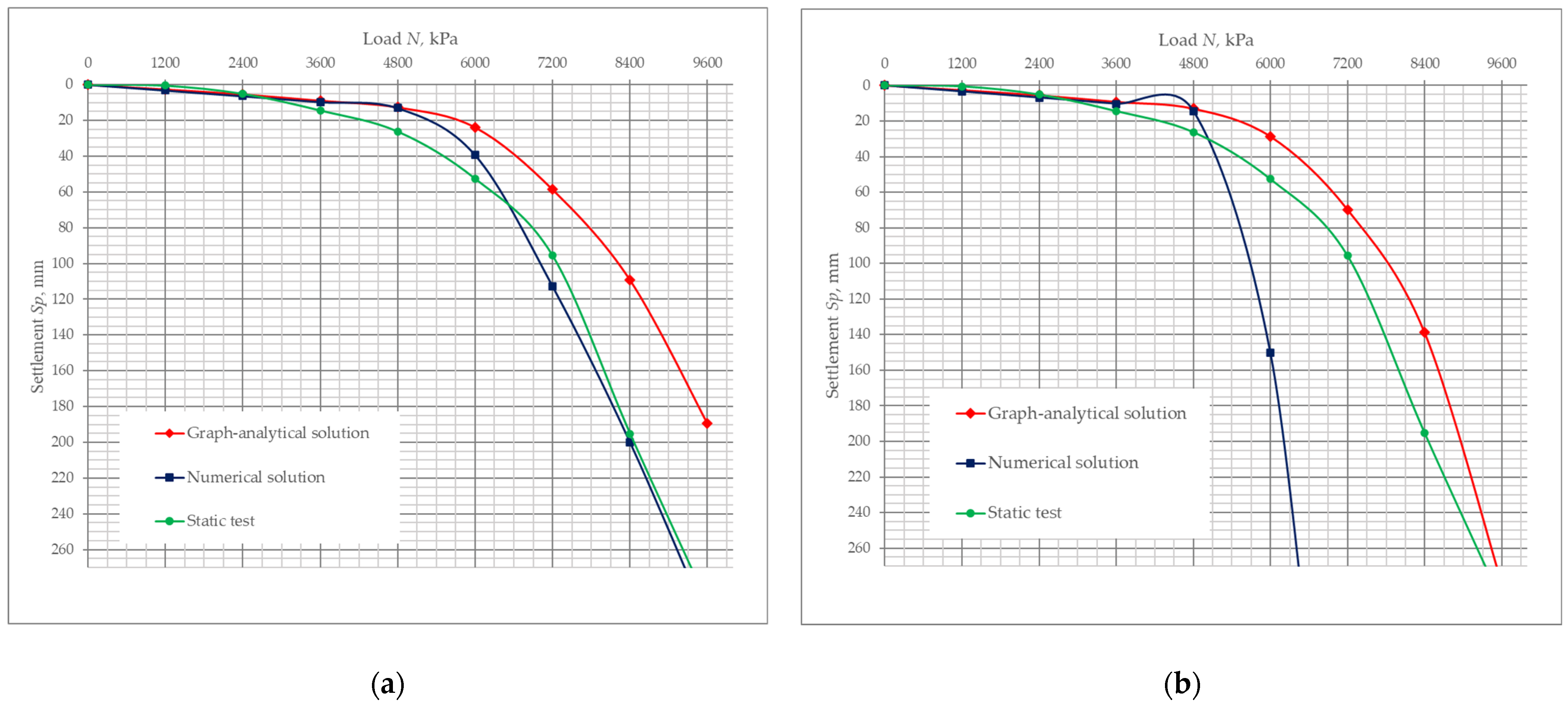
- A comparison of the graphs of the dependence of settlement on load obtained using the graph-analytical and numerical methods showed good convergence of the results. The maximum discrepancy of the settlement values was 12.9%, which does not exceed the engineering accuracy limit of 15%, indicating that this method can be used for calculations. In addition, a similar characteristic of deformation of the graphs is observed, and pile failure occurs at the same load value—2600 kN.
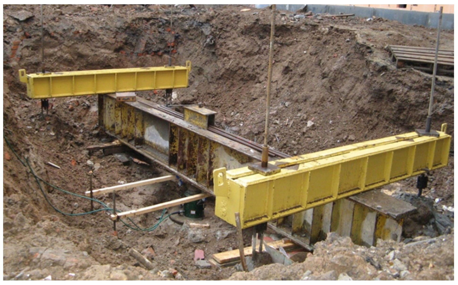
- Verification of the proposed graph-analytical method with the results of static pile testing showed that without the use of the strength reduction factors that reduce the strength of the contact zone soils, the graphs have a similar deformation character, but the calculated settlement values are less than the actual ones. The use of the strength reduction factors of 0.9 for loams and 1.0 for sands brought the calculated settlement values obtained by the graph-analytical method closer to the actual values. This indicates that these factors should be taken into account in the calculations.
- For a more accurate prediction of the settlement of a single pile calculated using the graph-analytical method, it is recommended to determine the strength reduction factors experimentally, either with laboratory tests or static tests of pile analogues, in similar engineering–geological conditions. In addition, in order to use the graph-analytical method of calculation in engineering practice, it is necessary to perform a larger number of calculations and compare it with the results of field tests of piles.
Author Contributions
Funding
Institutional Review Board Statement
Informed Consent Statement
Data Availability Statement
Acknowledgments
Conflicts of Interest
References
- Kurguzov, K.V.; Fomenko, I.K.; Sirotkina, O.N. Assessment of the bearing capacity of piles. Calculation Methods and Problems. Bull. Tomsk. Polytech. Univ. Geo Assets Eng. 2019, 330, 7–25. [Google Scholar]
- Polishchuk, A.I.; Samarin, D.G.; Filippovich, A.A. Estimation of the bearing capacity of piles in clayey soils with the help of PLAXIS 3D FOUNDATION PC. Vestn. TSASU 2013, 3, 351–359. [Google Scholar]
- Znamenskiy, V.V.; Ruzaev, A.M.; Poly’nkov, I.N. Comparison of the results of the field experiments with the calculations made with the finite-element program PLAXIS 3D FOUNDATION for the driven piles in the clayey soils. Vestnik MGSU 2008, 2, 18–23. [Google Scholar]
- Pilyagin, A.V. Design of Bases and Foundations of Buildings and Structures, 3rd ed.; revised and supplemented; ASV: Moscow, Russia, 2017; p. 398. [Google Scholar]
- Gotman, A.L.; Gavrikov, M.D. Investigation of the peculiarities of vertically loaded long bored piles and their calculation. Constr. Geotech. 2021, 12, 72–83. [Google Scholar] [CrossRef] [PubMed]
- Ter-Martirosyan, Z.G.; Sidorov, V.V.; Strunin, P.V. Theoretical bases of calculation of deep foundations—Piles and barretts. Vestn. PNIPU Constr. Archit. 2014, 2, 190–206. [Google Scholar]
- Ter-Martirosyan, Z.G.; Sidorov, V.V.; Strunin, P.V. Calculation of the stress-strain state of a single compressible barrette and pile at interaction with the soil massif. Zhilishchnoye Stroit. 2013, 9, 18–21. [Google Scholar]
- Ter-Martirosyan, Z.G.; Nam, N.Z. Interaction of long piles with two-layer elastic-crawling foundation. Bull. Civ. Eng. SPbGASU 2007, 1, 52–55. [Google Scholar]
- Ter-Martirosyan, Z.G.; Nam, N.Z. Interaction of long-length piles with inhomogeneous massif taking into account nonlinear and rheological properties of soils. Vestnik MSCU 2008, 2, 3–14. [Google Scholar]
- Victória, F.R.; da Costa, V.F.R.; Araújo, É.d.R. An elastic-viscoplastic load-transfer method for a single pile and pile groups. In Proceedings of the Joint XLII Ibero-Latin-American Congress on Computational Methods in Engineering and III Pan-American Congress on Computational Mechanics, Rio de Janeiro, Brazil, 9–12 November 2021; ABMEC-IACM: Rio de Janeiro, Brazil, 2021. [Google Scholar]
- Lapidus, L.S.; Lapshin, F.K. Bearing capacity of a pile immersed in a leading hole. In Mechanics of Soils, Bases and Foundations; Reports to the XXVII Scientific Conference; Routledge: Abingdon, UK, 1968. [Google Scholar]
- O’Neill, M.W.; Resse, L.C. Behaviour of axially loaded drilled shafts in Beaumont clay. In Research Report 89.8. Center for Highway Research; The University of Texas at Austin: Austin, TX, USA, 1970; p. 749. [Google Scholar]
- Balysh, A.V.; Sernov, V.A. Mechanical models of interaction of bored piles with the foundation. In Proceedings of the Geotechnics of Belarus: Science and Practice: Proceedings of the International Conference, Minsk, Belarus, 23–26 October 2018; Belarusian National Technical University: Minsk, Belarus, 2018; pp. 69–74. [Google Scholar]
- Thasnanipan, N.; Maung, A.W.; Aue, Z.Z. Record load test on a large barrette and its performance in the layered soils of Bangkok. In Proceedings of the 5th International Conference on Deep Foundation Practice Incorporating Piletalk International, Singapore, 4–6 April 2001. [Google Scholar]
- Ishihara, K. Recent advances in pile testing and diaphragm wall construction in Japan. Geotech. Eng. 2010, 41, 97–122. [Google Scholar]
- Nam, N.Z. Interaction of Bored Piles with the Soil Base with Consideration of Time Factor: Cand.Sci./Nguyen Zang Nam.-M.: MGSU. 2008, p. 167. Available online: https://www.dissercat.com/content/vzaimodeistvie-buronabivnykh-dlinnykh-svai-s-gruntovym-osnovaniem-s-uchetom-faktora-vremeni/read (accessed on 26 September 2007).
- Kravtsov, V.N. Investigation of limit states on bearing capacity and deformations of clayey bases of short ready-made (driven) piles of small cross-section at their pushing in and pulling out. Constr. Appl. Sci. Constr. Archit. 2021, 8, 65–74. [Google Scholar]
- Vasenin, V.A. Numerical modeling of testing of bored piles and baretta for construction of a high-rise building in St. Petersburg. Geotechnika 2010, 5, 38–47. [Google Scholar]
- Grigorian, A.A. Pile Foundations for Buildings and Structures in Collapsible Soils; Oxford IBH Publishing Co.Pvt.Ltd.: New Delhi, India, 1997; p. 153. [Google Scholar]
- Grigoryan, A.A. About a new mechanism of foundation failure on clayey soils under the foundations of structures. OFMG 2009, 3, 10–14. [Google Scholar]
- Nam, D.H. Interaction of Long Piles with the Soil in a Pile Foundation: Dissertation…Candidate of Technical Sciences: 05.23.02/Dinh Hoang Nam.—M. 2006. Available online: https://www.dissercat.com/content/vzaimodeistvie-dlinnykh-svai-s-gruntom-v-svainom-fundamente/read (accessed on 18 April 2006).
- Shulyatiev, O.A.; Dzagov, A.M.; Minakov, D.K. Change of stress-strain state of soil massif as a result of bored pile and baretta device. Vestn. SIC Stroit. 2022, 34, 26–44. [Google Scholar] [CrossRef]
- Potyondy, J.G. Skin friction between various soils and construction materials. Geotechnique 1961, 11, 339–353. [Google Scholar] [CrossRef]
- Eid, H.T.; Amarasinghe, R.S.; Rabie, K.H.; Wijewickreme, D. Residual Shear Strength of Fine-Grained Soils and Soil–Solid Interfaces at Low Effective Normal Stresses. Can. Geotech. J. 2015, 52, 198–210. [Google Scholar] [CrossRef]
- Kishida, H.; Uesugi, M. Tests of the interface between sand and steel in the simple shear apparatus. Géotechnique 1987, 37, 45–52. [Google Scholar] [CrossRef]
- DeJong, J.T.; Frost, J.D.; Saussus, D.R. Measurement of Relative Surface Roughness at Particulate-continuum Interfaces. J. Test. Eval. 2002, 30, 8–19. [Google Scholar] [CrossRef]
- Yin, K.; Fauchille, A.-L.; Di Filippo, E.; Kotronis, P.; Sciarra, G.A. Review of sand–clay mixture and soil–structure interface direct shear test. Geotechnics 2021, 1, 260–306. [Google Scholar] [CrossRef]
- Isaev, O.N.; Sharafutdinov, R.F. Investigations of soil shear resistance along the contact surface of structures. OFMG 2020, 2, 23–29. [Google Scholar]
- De Gennaro, V.; Frank, R. Elasto-plastic analysis of the interface behaviour between granular media and structure. Comput. Geotech. 2002, 29, 547–572. [Google Scholar] [CrossRef]
- Hu, L.; Pu, J.L. Application of damage model for soil–structure interface. Comput. Geotech. 2003, 30, 165–183. [Google Scholar] [CrossRef]
- Hu, L.; Pu, J.L. Testing and modeling of soil-structure interface. J. Geotech. Geoenvironmental Eng. 2004, 130, 851–860. [Google Scholar] [CrossRef]
- Liu, H.; Song, E.; Ling, H.I. Constitutive modeling of soil-structure interface through the concept of critical state soil mechanics. Mech. Res. Commun. 2006, 33, 515–531. [Google Scholar] [CrossRef]
- Saberi, M.; Annan, C.D.; Konrad, J.M. A unified constitutive model for simulating stress-path dependency of sandy and gravelly soil–structure interfaces. Int. J. Non-Linear Mech. 2018, 102, 1–13. [Google Scholar] [CrossRef]
- Saberi, M.; Annan, C.D.; Konrad, J.M. On the mechanics and modeling of interfaces between granular soils and structural materials. Arch. Civ. Mech. Eng. 2018, 18, 1562–1579. [Google Scholar] [CrossRef]
- Hu, Y.N.; Ji, J.; Sun, Z.B.; Dias, D. First order reliability-based design optimization of 3D pile-reinforced slopes with Pareto optimality. Comput. Geotech. 2023, 162, 105635. [Google Scholar] [CrossRef]
- Gong, W.; Tang, H.; Juang, C.H.; Wang, L. Optimization design of stabilizing piles in slopes considering spatial variabilit. Acta Geotechnica 2020, 15, 3243–3259. [Google Scholar] [CrossRef]
- Huang, Y.; He, Z.; Yashima, A.; Chen, Z.; Li, C. Multi-objective optimization design of pile-anchor structures for slopes based on reliability theory considering the spatial variability of soil properties. Comput. Geotech. 2022, 147, 104751. [Google Scholar] [CrossRef]
- Doroshkevich, N.M.; Znamenskiy, V.V.; Kudinov, V.I. Engineering methods of the pile foundations calculation at different schemes of their loading. Vestnik MSCU 2006, 1, 119–132. [Google Scholar]
- Glazachev, A.O. Experimental investigations of the vertically loaded small-scale bored piles. Vestnik MSCU 2014, 4, 70–78. [Google Scholar]
- Hansen, J.B. Revised and extended formula for bearing capacity. In Bulletin 28; Danish Geotechnical Institute: Copenhagen, Denmark, 1970; pp. 5–11. [Google Scholar]
- Verruijt, A. An Introduction to Soil Mechanics; Springer International Publishing AG: Dordrecht, The Netherlands, 2018; p. 420. [Google Scholar]
- GOST 12248.1-2020 Soils. Determination of Strength Parameters by Shear Strength Testing. Available online: https://protect.gost.ru/document.aspx?control=7&id=239175 (accessed on 1 January 2021).


| Soil | Unit Weight γ, kN/m3 | Modulus of Elasticity/Deformation E, MPa | Poisson’s Ratio ν | Cohesion c, kPa | Internal Friction Angle φ, deg |
|---|---|---|---|---|---|
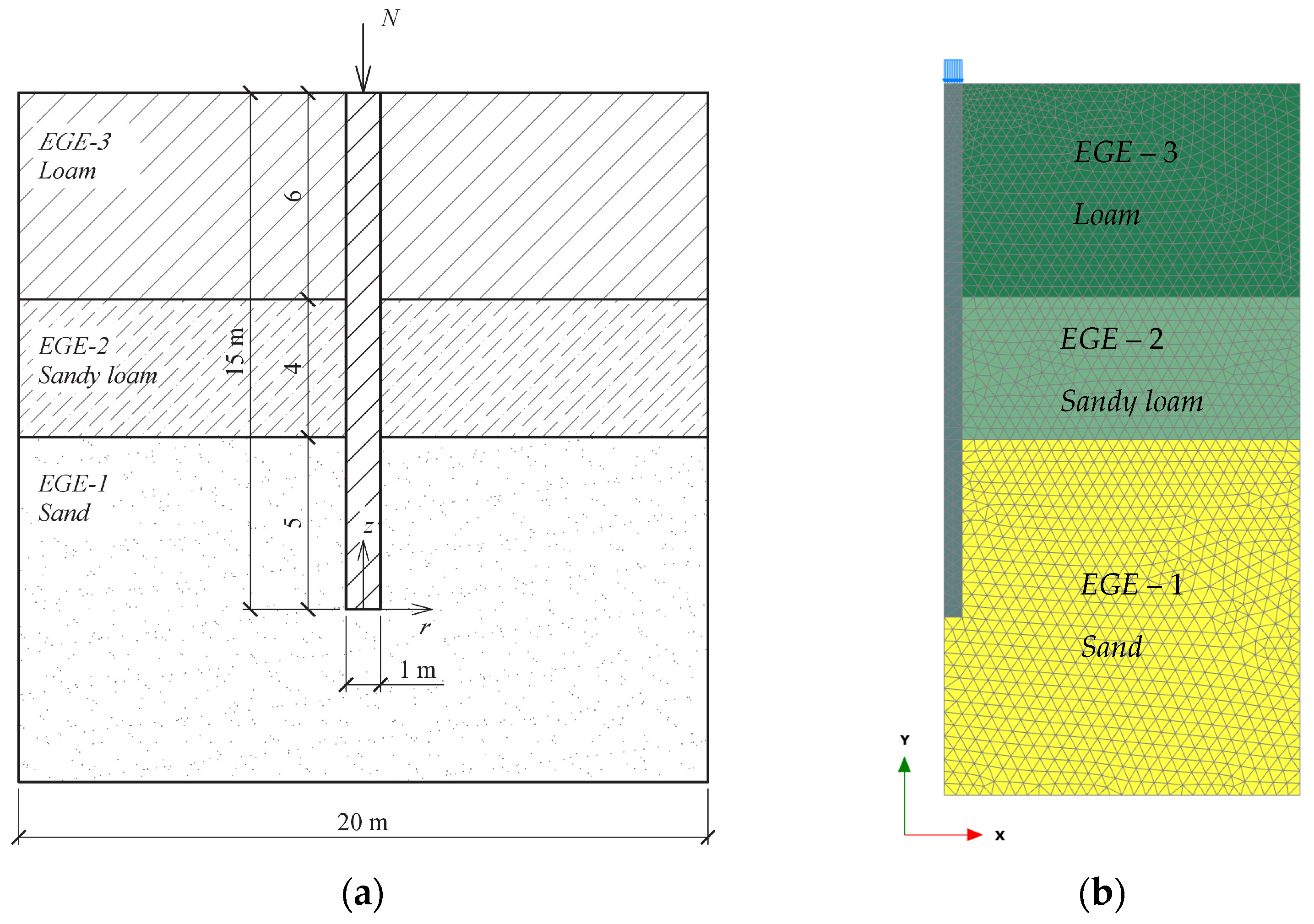
| EGE-3 Loam | 19.5 | 16.0 | 0.36 | 22 | 20 |
| EGE-2 Sandy loam | 19.6 | 13.0 | 0.36 | 16 | 15 |
| EGE-1 Sand | 18.0 | 21.1 | 0.30 | 1 | 30 |
| Concrete | 24.0 | 30 · 103 | 0.20 | - | - |
| № EGE | Soil | Unit Weight γ, kN/m3 | Modulus of Elasticity/Deformation E, MPa | Cohesion c, kPa | Internal Friction Angle φ, deg |
|---|---|---|---|---|---|
| 4, 10 | Soft-firm and very soft-firm loam | 19.9 | 9 | 7 | 20 |
| 13 | Fine sand | 20.5 | 28 | 3 | 33 |
| 14 | Sandy silt | 20.3 | 30 | 4 | 31 |
| 16 | Stiff loam | 19.9 | 28 | 29 | 20 |
| Soil | Plastic Limit WP, % | Liquid Limit WL, % | Plasticity Index IP | Shear Rate V, mm/min |
|---|---|---|---|---|
| Very stiff clay | 45 | 90 | 0.45 | 0.005 |
| Very stiff loam | 28 | 44 | 0.16 | 0.05 |
Disclaimer/Publisher’s Note: The statements, opinions and data contained in all publications are solely those of the individual author(s) and contributor(s) and not of MDPI and/or the editor(s). MDPI and/or the editor(s) disclaim responsibility for any injury to people or property resulting from any ideas, methods, instructions or products referred to in the content. |
© 2024 by the authors. Licensee MDPI, Basel, Switzerland. This article is an open access article distributed under the terms and conditions of the Creative Commons Attribution (CC BY) license (https://creativecommons.org/licenses/by/4.0/).
Share and Cite
Ter-Martirosyan, A.Z.; Sidorov, V.V.; Almakaeva, A.S. Graph-Analytical Method for Calculating Settlement of a Single Pile Taking into Account Soil Slippage. Appl. Sci. 2024, 14, 8064. https://doi.org/10.3390/app14178064
Ter-Martirosyan AZ, Sidorov VV, Almakaeva AS. Graph-Analytical Method for Calculating Settlement of a Single Pile Taking into Account Soil Slippage. Applied Sciences. 2024; 14(17):8064. https://doi.org/10.3390/app14178064
Chicago/Turabian StyleTer-Martirosyan, Armen Z., Vitalii V. Sidorov, and Anastasiia S. Almakaeva. 2024. "Graph-Analytical Method for Calculating Settlement of a Single Pile Taking into Account Soil Slippage" Applied Sciences 14, no. 17: 8064. https://doi.org/10.3390/app14178064
APA StyleTer-Martirosyan, A. Z., Sidorov, V. V., & Almakaeva, A. S. (2024). Graph-Analytical Method for Calculating Settlement of a Single Pile Taking into Account Soil Slippage. Applied Sciences, 14(17), 8064. https://doi.org/10.3390/app14178064