Abstract
The analysis and planning of suburban traffic flows is an extremely important task to ensure efficient and fluent traffic distribution in existing infrastructure. One of the main sources of this information from existing situations is origin–destination (OD) matrices, usually obtained from traffic CCTV cameras. In this paper, a novel method is proposed for the filtration of transit traffic from the overall traffic through the area. The main feature that differentiates this method from existing outlier (and thus transit traffic) detection methods is that it is focused solely on prolonged trips (which are believed to be caused by vehicles stopping in the investigated area). Initial calibration of the method on training data (sample size of N = 216,159 trips through paired detectors) and verification on test data prove the accuracy of the algorithm on the level of 98% in urban and suburban areas, respectively, in Czech Republic conditions, which gives high hopes for the feasibility of the method.
1. Introduction
The increasing challenges posed by a growing global population have increased the complexity of transportation systems, necessitating effective transit traffic filtration strategies in various regions. Transit traffic filtration in traffic data analysis refers to the process of distinguishing between vehicles merely passing through a city and those that stop within it. This task enables the separation of the internal urban traffic flow from the external vehicle entry, allowing a more accurate analysis of the dynamics of city traffic. The critical need for efficient management of transit traffic comes from widespread problems of congestion, environmental degradation, and energy consumption that hinder the effectiveness of mobility networks. These challenges span urban, highway, and rural areas, underscoring the importance of transit traffic filtration in understanding traffic structure in regions. This, in turn, leads to various benefits such as alleviating congestion, reducing travel times, minimizing fuel consumption, and mitigating environmental impact, as noted by Qi et al. [1].
In densely populated urban settings, the filtration of transit traffic plays a key role in addressing the intricate dynamics of mobility. Beyond mere functionality, it contributes to improving the quality of life of urban residents [2], aligning with the broader objective of creating environmentally friendly and livable cities through more effective urban traffic planning tools.
Rural areas, although distinct, are not exempt from transit traffic challenges. Identifying and filtering transit traffic in rural settings is crucial to maintaining accessibility and connectivity. Sustainable transportation practices in these regions contribute to the preservation of the landscape and mitigate the environmental impact of transportation activities. At the same time, they contribute significantly to the daily traffic conditions in cities [3].
Highways, as critical connectors between regions, face challenges of congestion. Effective highway traffic filtration involves understanding long-distance travel dynamics, optimizing traffic flow, and considering economic implications. This approach not only facilitates smoother travel experiences but also improves the economic vitality of regions interconnected by highways.
The analysis of the current state of the art suggests that there is a lack of significant research focused specifically on the identification and filtration of transit traffic from overall origin–destination data. The vast majority of studies focus on the identification of real travel time for forecast or navigation purposes. These two tasks, although similar, have different goals and thus results. The method proposed in the subsequent chapters of this work is focused on the filtration of outliers based on travel time data rather than unveiling the true travel time.
The insights derived from this research provide a tool for establishing evidence-based policies tailored to the specific needs of urban, highway, and rural settings. Policymakers can leverage these findings to develop targeted strategies that optimize regional mobility, reduce environmental impact, and improve the efficiency of transportation systems.
The further structure of this paper introduces the most common methodologies found in the current literature, proposes a transit identification and filtration algorithm, and verifies real-world data collected in Czech Republic urban, rural, and highway traffic. The results of this research have multiple contributions to the current state of the art in the field of transport planning and management, by enabling data-driven decision making for future policy and traffic planning.
2. Literature Review
The first references to the utilization of outlier filtering techniques to acquire valid travel time measurements in matched license plate data were made in 1983. Fowkes [4] proposed a median and quartile statistic, mentioning that it is more robust to the detection of outliers than the mean and standard deviation. Montgomery and May [5] used a two-step process to eliminate outliers while researching variability in travel time on Leeds’s arterial roads. In the beginning, a high cutoff value was established to remove any extreme values. Subsequently, median and quartile measures were applied to the cropped data to create a confidence interval in which valid travel time observations could be found. The main conclusion of this study was the necessity to effectively remove outliers from travel time data for their effective analysis.
Clark et al. [6] followed up on previous research by summarizing three statistical approaches to filtering travel times obtained from matched license plate data and aggregated in 5 min intervals. The first approach is based on the use of the first and ninth deciles to identify outlying travel times. The second involves the use of the mean absolute deviation (MAD) test. Travel times are considered valid if they are located within a confidence interval, which is set to be three times the MAD in the evaluated time period. However, Robinson and Polak [7] argued that ‘mean absolute deviation is sensitive to the presence of outliers, it may be preferable to use a more robust measure of range, such as the interquartile range’. The final approach proposed a standardized normal z- or t-test using the median and quartile deviation. This approach uses a series of correction factors, as the standard tabulated multipliers are not appropriate, as variance of the median is not the same as that of the mean. Clark et al. [6] discuss that the percentile approach is too extreme, since it always classifies 20% of the data as outliers. The MAD and the standardized test produce a similar percentage of detected outliers, but the standardized test is considered more robust to outliers.
Dion and Rakha [8] discuss the use of outlier detection methods in systems that provide travelers with real-time travel time estimates. Such systems include the TranStar system in Houston [9], the TransGuide system in San Antonio [10], or the Transmit system in the New York metropolitan area [11]. Dion and Rakha [8] suggested that existing methods do not take into account sudden changes in travel times, so they proposed two versions of a low-pass filtering algorithm to estimate the average travel time on road links. This technique assumes that the travel times in the 5 min intervals have a log-normal distribution. The first version of the algorithm uses the mean and standard deviation to create a confidence interval in which the valid travel times are located. In addition to the aforementioned methods, Dion and Rakha extended the method in the second version by considering that the third of three consecutive travel time observations is valid if the three observations are either above or below the range of the constructed confidence interval.
Robinson and Polak [7] proposed an overtaking rule method to clean matched license plate data. This approach is based on the assumption that vehicles with valid travel time are unlikely to pass on a single-lane road, and if on a multilane road, the difference in travel time between itself and the overtaking vehicles would not be too great. Robinson and Polak used Vissim, a micro-simulation software, to collect their travel time data, which allowed them to calculate the population mean and standard deviation of valid travel times. However, the method is highly dependent on a parameter called tolerance time, which is hard to obtain since one is required to know the distribution of valid travel times. Robinson and Polak [7] state that as the tolerance time increases, the number of vehicles falsely classified as valid will increase.
Zheng et al. in [12] introduced an algorithm based on the fuzzy c-line clustering method developed by Bezdek [13]. The algorithm assigns a measure of membership to each travel time observation, which is then used to create a fuzzy line prototype. The weighted average of travel times is then calculated, with the weight being the degree of membership in the fuzzy line prototype. Nevertheless, a prior knowledge of outliers’ values is required as input to this algorithm, rather than a result which is in contradiction to this study.
Moghaddam and Hellinga [14] used data from a Bluetooth detector instead of matching license plates to develop an outlier detection algorithm. Since license plates are used as unique vehicle identifiers, the use of the MAC address of the Bluetooth device seems viable. The proposed algorithm is based on creating a confidence interval that is determined by the expected mean and standard deviation in the current time interval evaluated, as well as the distribution of individual travel times in the preceding time interval. This leads to a complex quasi-prediction process to evaluate the expected mean and standard deviation based on the latest available travel time estimates.
In 2016, Jang [15] proposed an algorithm that evaluates the number of observations in the current time interval and then determines the confidence interval based on the previous time interval or the current. The algorithm utilizes the median absolute deviation to construct the confidence interval if the number of observations is greater than three. If the number of observations is not enough, the algorithm uses the confidence interval created from the previous time interval. Although similar to the Clark et al. [6] MAD test, this approach introduces a new element by comparing the medians obtained from the current and previous time intervals to form the confidence interval. The weakness of this approach is the dependence on a large number of user-defined parameters, creating the necessity for robust manual calibration [16].
Finally, Li et al. [17] employed a wavelet analysis technique to clean the travel times acquired from the matched license plate data. This technique used Daubechies wavelets at level 4 to identify the approximation and detail coefficients. These coefficients were then used to reconstruct travel time series, which were further compared to the travel time data obtained. An observation of travel time was considered an outlier if the difference between the obtained and reconstructed travel times was larger than the standard deviation of these differences in the entire data set. Li et al. [17] discussed that this approach could depend on the type of wavelet or the level of decomposition.
Despite advances, each method has its own set of assumptions, advantages, and disadvantages, summarized in Table 1. Based on a comprehensive analysis of existing methodologies, a critical need arises for a new algorithm that universally addresses a wide variety of travel time scenarios and enables the classification of through traffic without an extensive calibration process for each measurement site. Although the analyzed algorithms present a fairly powerful method to unravel the true underlying travel time on the analyzed routes, they are not free from certain drawbacks. Firstly, all of them aim to filter travel time by disregarding positive and negative outliers. This, in a natural way, assumes that there is some statistical mean value of the time needed to travel from the origin to the destination. As a consequence, vehicles traveling faster and slower than this mean value (and some tolerance value) are treated as error values (outliers). This approach is invalid for transit traffic filtration (identification and removal of vehicles traveling with some mid-stop between origin and destination), as it also eliminates vehicles that travel faster. By assumption, transit traffic has to travel slower. This difference in the philosophy of outlier treatment seems straightforward but has far-reaching consequences. It is often of crucial importance to know the volume of transit traffic as accurately as possible for traffic organization purposes. Secondly, the existing algorithms all assume extensive calibration before the use of the said algorithms on each separate route. This puts high demands on the manual labor of regional traffic experts who know the characteristics of the traffic in the regions studied. The limitations identified in current approaches underscore the need for a more adaptive and robust algorithm, one capable of responding to abrupt changes in travel times and accommodating the dynamic nature of traffic scenarios without the need for additional calibration.

Table 1.
A summary of the most prominent transit traffic filtration algorithms found in the literature.
3. Materials and Methods
To overcome the basic assumptions and relative merits associated with current algorithms to classify transit travel times, a new method is proposed based on the statistical analysis of measured travel times in the collected origin–destination pairings. It is vital to highlight here that the proposed method is not aiming at true travel time estimation but rather filtration of the travels with intermediate stops between origin–destination pairings for the purpose of transit traffic counting and analysis. To ensure a clear representation of the steps performed, this section is divided into three parts, first illustrating the overall workflow of method development and then describing the proposed method with a focus on mathematical and statistical operations involved in the algorithm. Lastly, the final subsection is dedicated to a description of the verification methods of the proposed method.
3.1. Framework for Algorithm Development and Verification
To develop and validate the proposed method, a data set collected over a 3-year period was used by dedicated efforts of the Czech Technical University in Prague, Faculty of Transportation Sciences. The initial data set was derived from 16 different origin–destination traffic surveys conducted between 2020 and 2022. These traffic surveys focused on evaluating the volume of transit traffic in urban or suburban areas of the Czech Republic. Data were collected methodically using Automatic Number Plate Recognition (ANPR) cameras during the day, in 12 h periods. Each survey consisted of several locations for data collection. The origin–destination pairs were then identified based on vehicle timestamps indicative of the routes traveled by the detected vehicles. Temporal alignment of records allowed for reconstruction of vehicle routes. From the data analyzed, 6643 origin–destination pairs were obtained, which captured a diverse range of real-world traffic scenarios, each influencing the travel times observed within the defined origin–destination pairs. Table 2 shows an example of the data set used for the paired vehicle travel times along a selected segment of the origin–destination pair.
Table 2.
Example of selected origin–destination pair segment vehicle travel times data set.
The origin–destination pairs predominantly showcased the travel times of vehicles that traveled on urban roads, with occasional inclusions of highway links. This heterogeneous environment resulted in a wide spectrum of travel times, depicting various traffic scenarios throughout the day. Most pairs exhibited stable travel times, reflecting consistent traffic flow throughout the monitored day. However, instances of congestion-induced increases in travel times, where temporary interruptions led to elevated travel times before returning to normal length, were observed throughout the day. These congestion-related events were observed during peak traffic hours and during the day, demonstrating the dynamic and stochastic nature of urban traffic patterns.
An example of temporary spikes in vehicle travel times was recorded in traffic accidents. Another instance involved a pair affected by road maintenance works, where traffic lights were used to manage vehicular movement in a single direction. This unique scenario introduced fluctuations in travel times, which further contributed to the diverse range of observed traffic patterns. The diverse nature of the data obtained and the variability in traffic scenarios, which includes both vehicles passing through and vehicles with partial destinations, proved to be highly problematic for the investigated existing solutions and therefore advocated for the development of the proposed algorithm.
For the development of the proposed algorithm, the main premise was the ability to perform repeated filtration of transit traffic, using self-calibration to travel times samples on different pairs of origin–destination locations without manual interference into the algorithm. For this purpose, an auto-regression analysis was implemented. Based on this, an algorithm developed in our research and presented in Section 3.2 consists of a part that serves as a self-calibration (repeated linear regression over short time intervals) and a cutoff part that treats all values that did not contribute to a significant change in root mean square error as transit traffic. Specific steps in the algorithm and numerical operations are presented in the form of pseudocode in Section 3.2.
3.2. Transit Traffic Filtration Algorithm
Given the shortcomings of existing travel time estimation methods and their symmetrical effect on outlier detection, a new algorithm (see Algorithm 1) is proposed. The primary motivation for designing this algorithm is the need to effectively filter out transit travel times, which are often misclassified by existing methods. The algorithms mentioned in Table 1 tend to overlook transit travel times or inadequately assume that non-transit travel times are actually transit, leading to inaccurate quantification of transit traffic volumes.
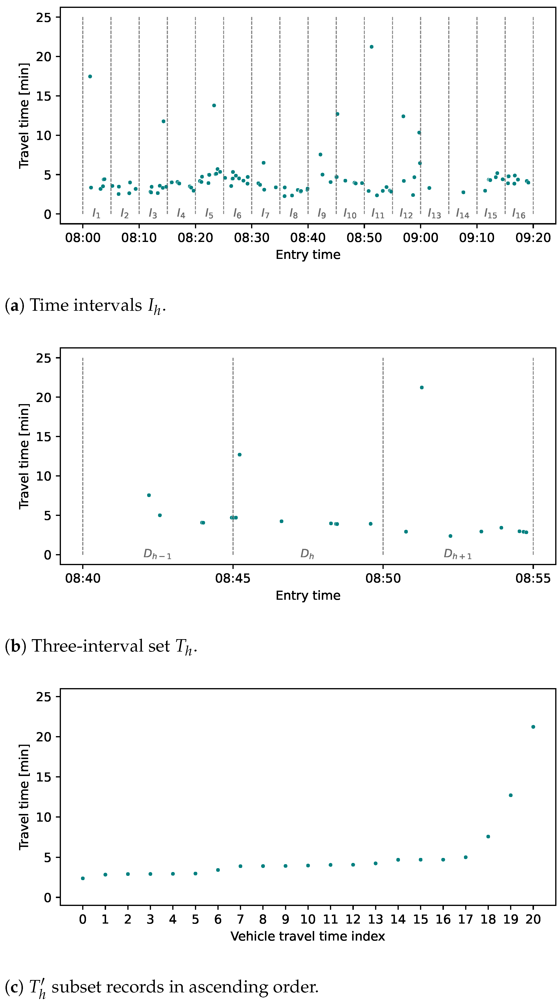
The proposed algorithm begins with the initialization process (line 1), where it establishes a temporal association by assigning time intervals, denoted , to each license plate record based on its entry timestamp. These intervals are defined by a start time and an end time , where is set to 5 min. The choice of is motivated by the insights obtained from the literature, described in Section 2, which suggest that shorter intervals help capture subtle variations in travel time behavior. This interval length is crucial for accurately reflecting the dynamics of traffic conditions, especially in environments where traffic can fluctuate rapidly. Next (line 2), for each interval , a set is formed, representing the travel time values of vehicles that travel along the origin–destination pair route within that time window (Figure 1a). This process ensures that the data are segmented into manageable chunks, allowing for a focused analysis on specific time windows, which is more effective in isolating outliers compared to global approaches that consider the entire data set at once.
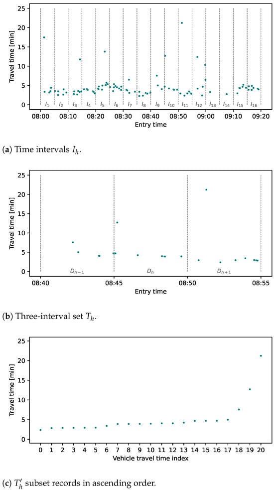
Figure 1.
and subsets created from time intervals.
Transitioning to the main loop (line 3), the algorithm forms a set of three intervals (Figure 1b) for each in the assessed data set (line 4). This three-interval structure is designed to capture the temporal context by considering travel times immediately preceding and following the current interval, providing a more holistic view of traffic conditions. This method addresses the drawback of earlier algorithms that only considered isolated intervals, which often led to misinterpretation of transient traffic patterns as outliers. The set includes the travel times of the previous interval , the current interval , and the subsequent interval . This structural arrangement was purposefully chosen to evaluate travel times around the time of the assessment, providing a wide perspective of the current state of traffic conditions. This segmentation aligns with the findings of several studies [6,8,12,14,15], which emphasize the importance of capturing dynamic travel time patterns within distinct temporal boundaries.
| Algorithm 1 Transit traffic filtration algorithm. |
|
Subsequently, in the main loop, we calculate the initial threshold value (line 5). This threshold is crucial in identifying potential outliers in shorter travel times by using the median and standard deviation of logarithmic travel times within the set , a method chosen to reduce the impact of these low values that could skew the analysis. These values are automatically classified as transit travel times. After determining the cutoff value , a subset (line 6) is created that retains only the travel times whose logarithmic values are greater than or equal to . This filtering step is implemented to exclude very small values, thereby ensuring that the selected travel times, when ordered in ascending order, show similarity and gradual increase, reflecting meaningful changes in travel time behavior. By ordering the travel times, the algorithm can better detect gradual shifts in travel time trends, which are often indicative of normal traffic conditions, as opposed to abrupt changes typically associated with stops. Note that by ordering the travel times in ascending order we lose information about the time sequence of travel time observations. However, this ordering is acceptable in our context because we evaluate the relationship between individual vehicles within 15-min time intervals, and the order of intervals is maintained by containing information about long-period travel time trends. This step improves computational efficiency while still preserving the integrity of the analysis by focusing on broader trends within discrete time intervals.
The algorithm then determines the number of remaining travel times, denoted as m, within the filtered subset (line 7). Then, these travel times are sorted (line 8) in ascending order (Figure 1c), resulting in a refined subset . This ordered representation allows for a more structured analysis of the underlying temporal patterns within the data set. This ordering is carried out due to the subsequent construction of a linear regression model during the iterative process in the inner loop of the algorithm that starts on line 9. It can be seen in Figure 1c that the ordered travel time records follow a linear pattern for the values that are similar to or close to each other. Using the values in the subset , the algorithm systematically builds a linear regression model for all data points up to the most recently added value in the latest iteration.
The rationale behind using a linear regression model is that it provides a straightforward and effective way to capture the expected linear relationship between consecutive travel times under normal traffic conditions. A significant deviation from this linearity would indicate an anomaly, such as a vehicle stopping, which is exactly what the algorithm aims to detect. The addition of a value that significantly deviates from the linear pattern of previous values would reflect a travel time different from that of vehicles passing through without stopping. As a result, this introduced value would alter the underlying linear pattern, leading to an increase in the root mean square error of the linear regression model calculated in step 10 of the algorithm. RMSE is calculated based on the actual travel time values and the expected travel time values obtained from the constructed linear regression line. The objective of this iterative procedure is to detect such changes in RMSE with the addition of new values, serving as an indicator of a potential deviation in travel time behavior. During each iteration, the between steps is updated on-line. The is set to 0.
The main loop iteration ends with the creation of a subset on line 17 that retains only the travel times of , where the absolute value of is less than . This final filtering step ensures that only travel times that closely conform to the expected linear pattern are considered valid, effectively removing outliers caused by non-transit traffic. The highest value of travel time within is identified as the cutoff travel time on line 18. This particular value is crucial as it establishes a threshold beyond which travel times are likely to represent vehicles that have stopped, thus addressing the limitations of previous methods that failed to accurately differentiate between transit and non-transit travel times. The cutoff travel time is then used (line 19) to filter the initial set , consisting of the travel times associated with the assessed time interval. In this way, we achieve the set , which consists of travel times identified by the algorithm as valid.
To initiate and complete the algorithm, two appropriate modifications are applied to construct and . In , the first interval is evaluated with two consecutive intervals and , due to the absence of prior travel time information. Similarly, in , the last interval is evaluated with the two preceding intervals and .
3.3. Verification of the Method
To facilitate the analysis and validation of the proposed algorithm, 120 origin–destination pairs were deliberately selected from the extensive data set to ensure the inclusion of examples representing stable flows, as well as fluctuations caused by congestion events, traffic accidents, and road maintenance. The selected origin–destination pairs were then divided into three different categories based on their inherent characteristics, one of which is the travel time pattern during the day. Traffic flow volume at 12 h in these selected pairs ranged from 180 to 10,000 vehicles, further contributing to the robustness of the data set used. The categories are represented by three example routes, named routes A to C, each showing distinct travel time patterns and the corresponding traffic scenarios.
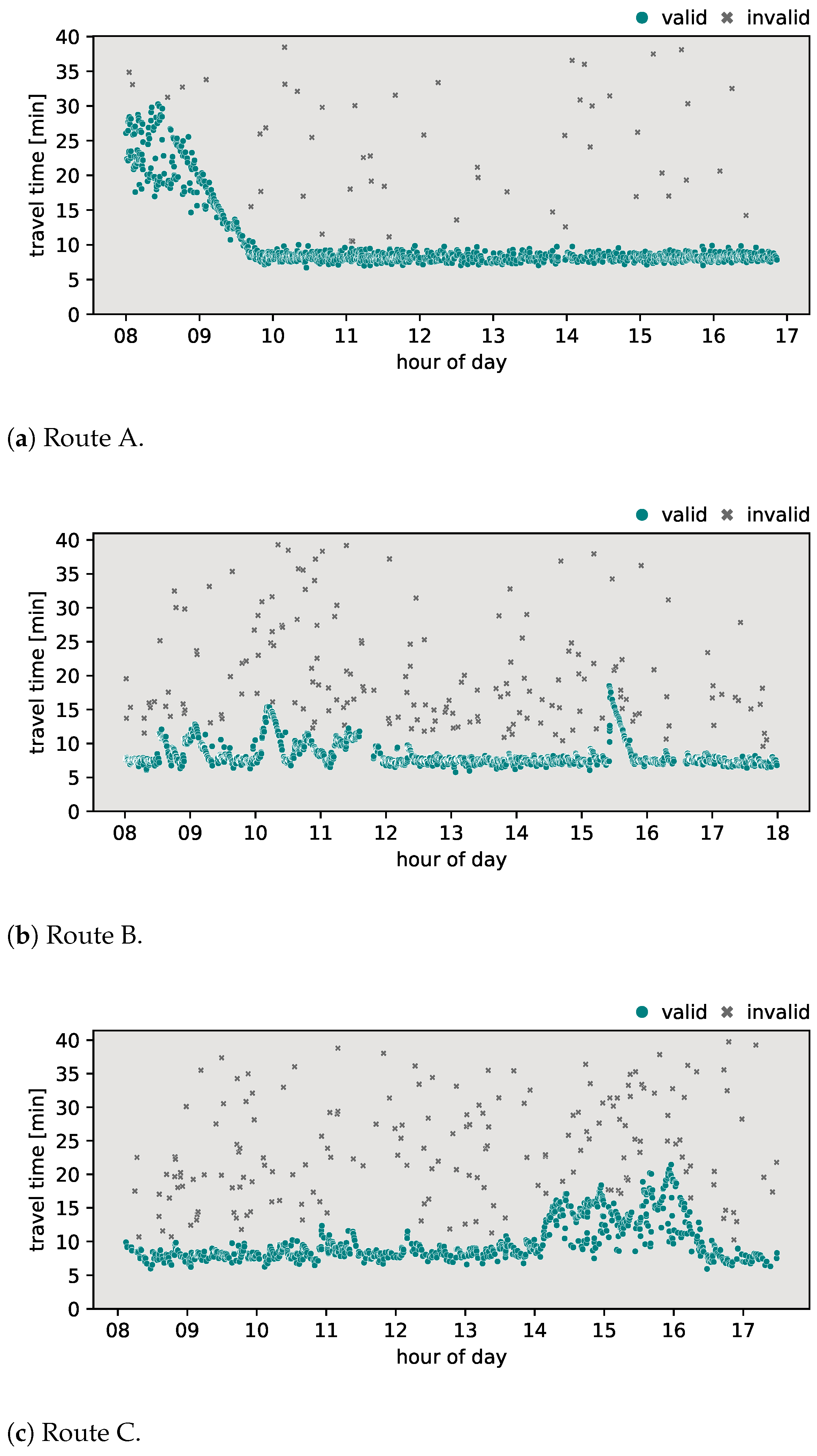
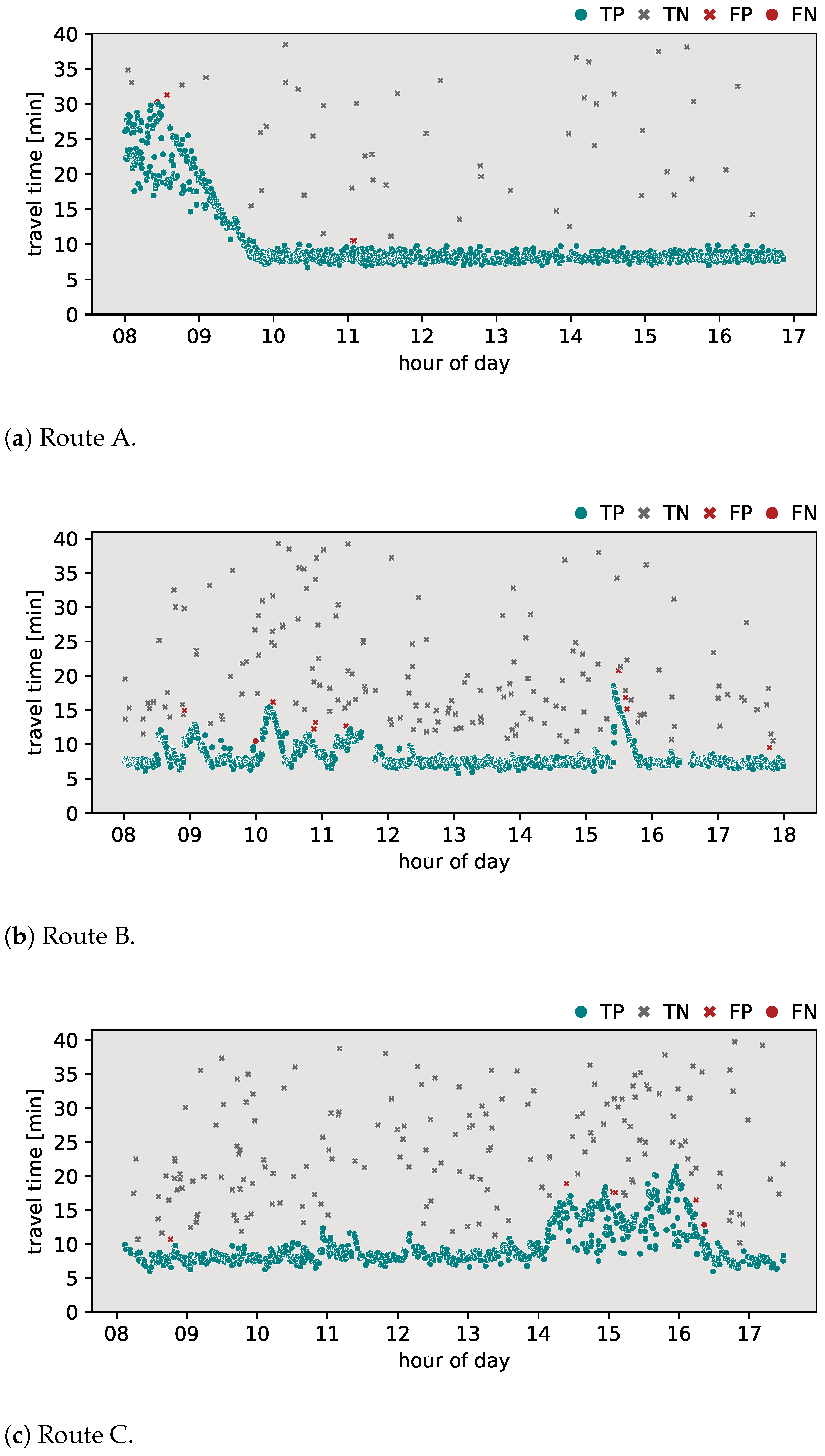
To assess the effectiveness and precision of the proposed algorithm, it was necessary to determine valid travel time values for each pair of origin–destination locations. Valid travel times between the origin–destination pairs, identified as ‘transit traffic’, represent vehicles that traveled from their origin location to their destination without stopping on the way. This process was carried out manually by the authors based on their domain-specific knowledge and expertise. The results of this initial classification can be seen in Figure 2.
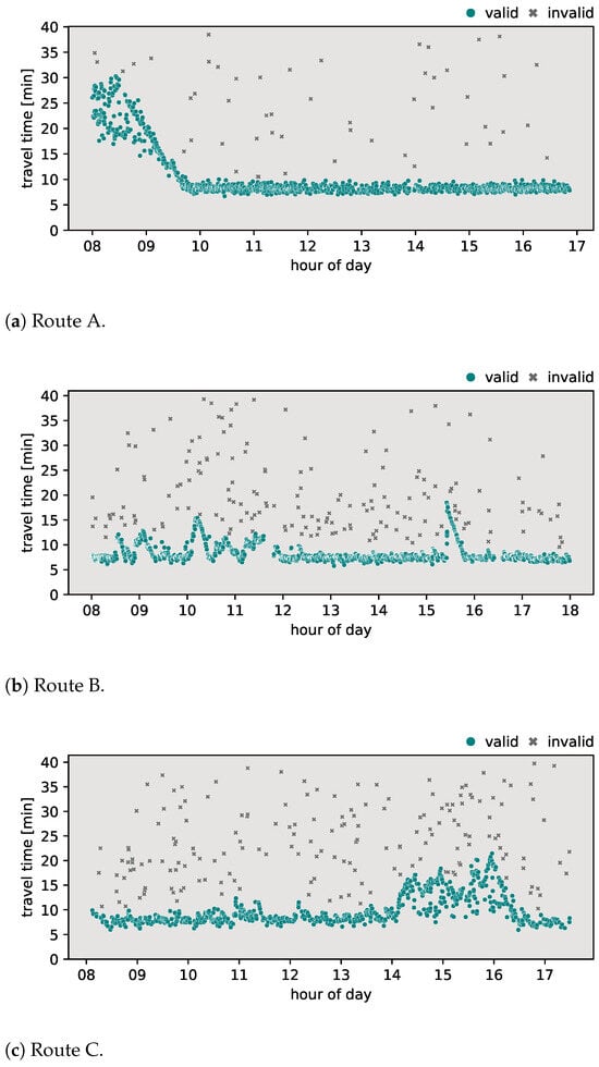
Figure 2.
Initially classified travel times on selected routes.
For the purpose of evaluating the new algorithm, four existing methods were chosen as the benchmark (the Jang algorithm, Dion–Rakha version 1, Dion–Rakha version 2, and the Robinson–Polak algorithm). The choice of these algorithms was motivated by their calibration difficulty and robustness in different traffic scenarios. As the purpose of this work is to create a robust tool for automated transit filtration without the need for extensive setup and calibration, other methods described in the Section 2 were deemed unfit for these conditions. The configuration of the internal parameters of the compared algorithms was in accordance with the recommended values in the literature [7,8,15]. As the algorithm’s objective was outlier classification, a comparative evaluation consisted of analyzing the confusion matrices generated from the results of each applied algorithm. These measures helped to assess the algorithm’s ability to correctly classify travel times and the instances of misclassification (false positives and false negatives). The -score metric, derived from the confusion matrix data, provided a single numerical value able to weigh sensitivity and accuracy according to the specific needs of each task, where the parameter indicates how many times sensitivity is more important than accuracy. Due to the emphasis on high sensitivity, the parameter was set to 2 for this task. This setting reflects the fact that sensitivity is twice as important as accuracy.
In order to evaluate the algorithm’s responsiveness to sudden fluctuations in travel times, the collected travel time data were plotted in the travel time–daytime domain (see examples in Figure 2). This visual analysis led to the identification of three different categories of routes (origin–destination pairings) that were used as testing data for the responsiveness of the proposed classification algorithm.
- Route A—urban arterial routeAn important feature of this route is an intersection with a directional ramp that facilitates the transition from a ring road to a main arterial road that enters the city. Other various exits along the route serve nearby residential and commercial areas, allowing vehicles to stop and thus observe non-transit travel times. Furthermore, the presence of a dedicated bus lane plays a key role in influencing travel times along this route, particularly during the morning peak hours. A visual analysis of Figure 2a shows that morning travel times peak at almost 30 min, reflecting the impact of capacity limitations due to infrastructure characteristics. After the morning rush hour, around 10 A.M., travel times stabilize at approximately 9 min, translating to an average speed of around 65 km per hour. The above-mentioned behavior can be seen on a graphical representation of the travel times plot during the morning rush hour.
- Route B—suburban commute routeCharacterized by a two-lane configuration with a single lane in each direction, overtaking is generally prohibited in most sections of this route. Two villages along the way with several pedestrian crossings contribute to reduced speeds. A notable feature is a single-lane roundabout with relatively high traffic flow, which could influence travel times along the route. In the visual examination presented in Figure 2b, morning travel times exhibit fluctuations ranging between 8 and 15 min, with sporadic data gaps during certain time periods. In the afternoon, a notable traffic accident occurred on this route, leading to longer travel times of up to 20 min. After the accident, travel times stabilize around 8 min in the afternoon, corresponding to an average speed of approximately 56 km per hour. This observation underscores the impact of external factors, such as accidents, on the temporal dynamics of travel times along route B.
- Route C—urban transit routeRoute C is characterized as a transit route through the city, featuring multiple intersections and notable points of interest, such as commercial and residential areas, along with the city center. A visual analysis of Figure 2c shows a relatively stable but oscillating pattern of travel times throughout the day. This minor variability can be attributed to the transit nature of the route, influenced by several major intersections that affect travel times. During the afternoon period, a more pronounced fluctuation is evident, particularly during rush hour. Some vehicles appear to have taken faster paths along this route, resulting in lower observed travel times compared to vehicles that followed the conventional path. Given that the route traverses the entire city, there are instances of non-transit vehicle travel times, which could reflect partial destinations within the city during their overall journey. Stable travel times along this route are consistently around 9 min, resulting in an average speed of 37 km per hour.
4. Results
In this section, the classification results of the proposed algorithm are provided. To further highlight the added value of the proposed method, a comparison was made with the most common methods currently applied in the field. The outlier detection algorithms discussed in Section 2 were applied to the travel time data sets for routes A, B, and C. Specifically, the algorithms evaluated include the Jang algorithm, the Dion–Rakha algorithm versions 1 and 2, and the Robinson–Polak algorithm. The classification results of these analyses are shown in Figure 3, Figure 4, Figure 5, Figure 6 and Figure 7. To provide a complete assessment, the confusion matrices along with the -score metric are presented in Table 3.
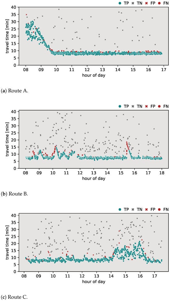
Figure 3.
Results of Jang algorithm.

Figure 4.
Results of Dion–Rakha v1 algorithm.
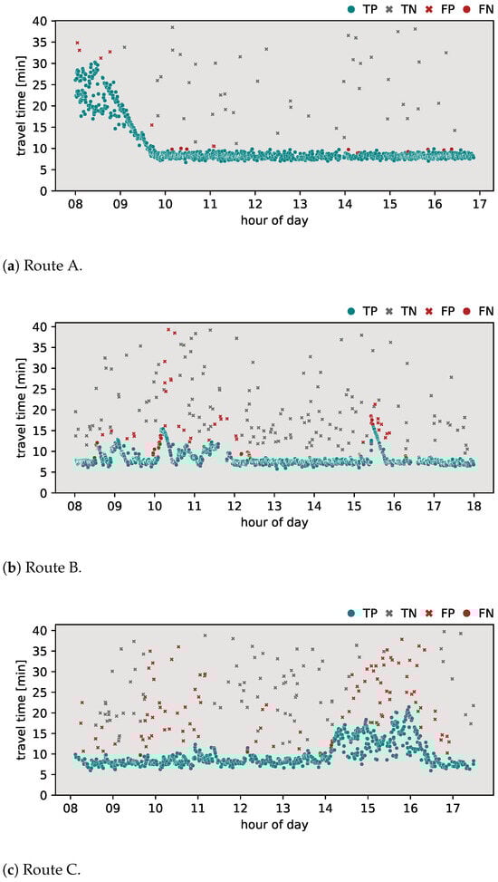
Figure 5.
Results of Dion–Rakha v2 algorithm.
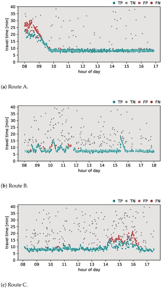
Figure 6.
Results of Robinson–Polak algorithm.
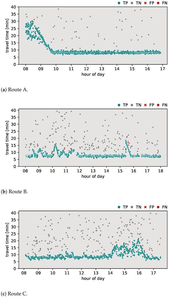
Figure 7.
Results of proposed algorithm.
Table 3.
Confusion matrices along with accuracy metrics of evaluated algorithms.
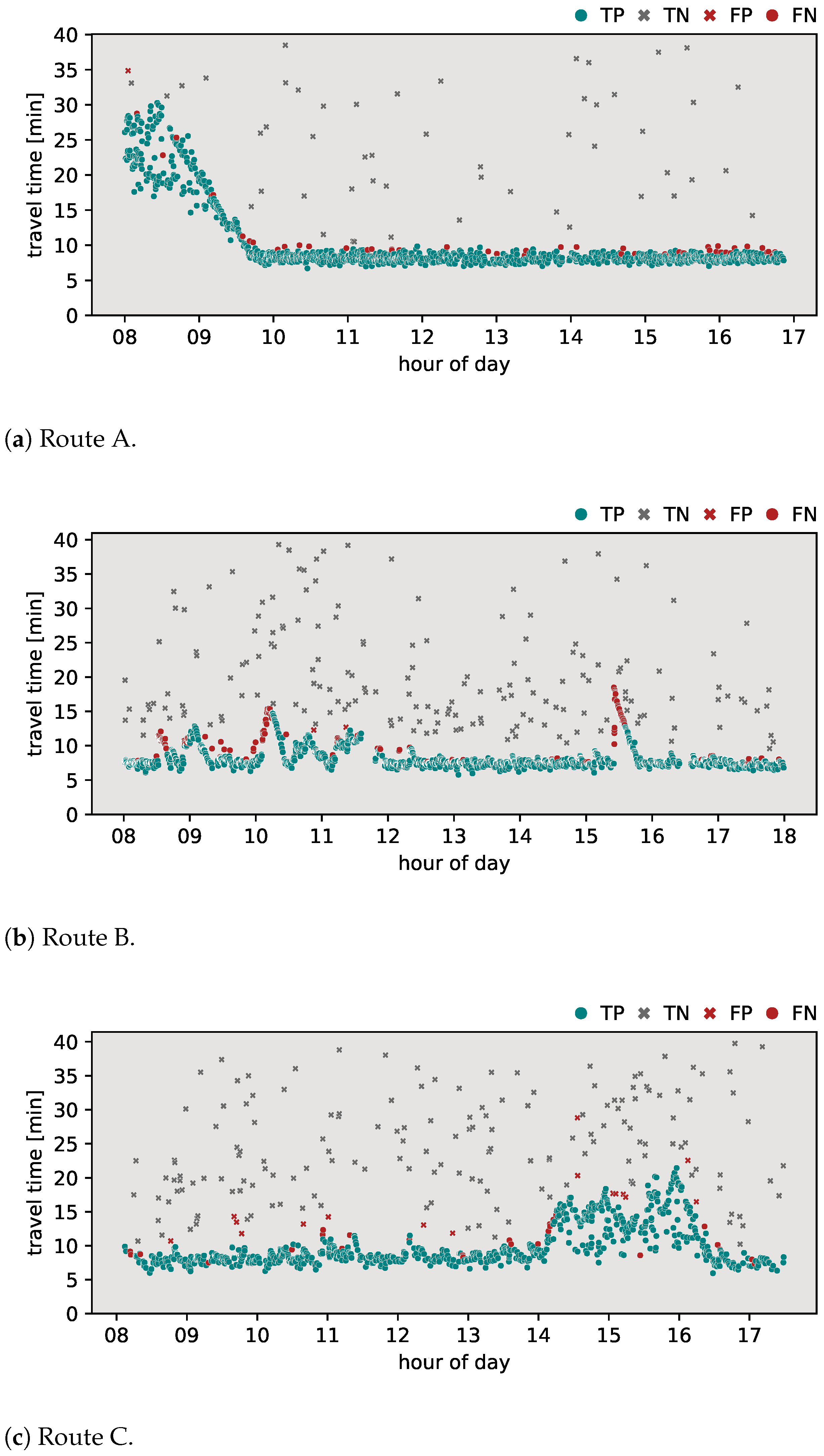
Figure 3 illustrates the classification results obtained using the Jang algorithm. On route A (Figure 3a), the algorithm demonstrated an -score of 0.933, with 47 false negatives (FNs) detected and only 1 false positive (FP) result. However, on route B (Figure 3b), the algorithm exhibited an -score of 0.812. A notable number of 259 FNs suggests difficulties in responding to sudden changes in travel time behavior. Similarly, when applied to route C (Figure 3c), the algorithm achieved an -score of 0.939. Despite this, it showed a relatively balanced distribution of falsely classified observations, with 18 FPs and 29 FNs. Positively, the algorithm demonstrated the ability to react to gradually increasing travel times.
Figure 4 shows the classification results obtained using the Dion–Rakha version 1 algorithm. On route A (Figure 4a), the algorithm performed with a commendable -score of 0.947, with a result of 7 detected FNs and 10 FPs. On route B (Figure 4b), the algorithm exhibited an -score of 0.724, with 42 FPs and 196 FNs, also suggesting difficulties in responding to sudden changes in travel time behavior. When applied to route C (Figure 4c), the algorithm achieved an -score of 0.802, with 74 FPs and 20 FNs. Despite its ability to capture gradually increasing travel times, the algorithm had difficulties establishing a valid travel time range in time intervals following abrupt changes, leading to a higher number of FNs.
Figure 5 presents the classification results obtained using the Dion–Rakha version 2 algorithm. In particular, for route A (Figure 5a), the algorithm produced results identical to those of the Dion–Rakha version 1 algorithm. On route B (Figure 5b), the algorithm achieved an -score of 0.763, with 38 FPs and 151 FNs. Although this algorithm showed fewer difficulties in responding to abrupt changes in travel times compared to version 1, it encountered similar challenges in establishing valid travel time ranges as the Dion–Rakha version 1 algorithm. Applying the algorithm to route C (Figure 5c) resulted in an -score of 0.697, the lowest of all algorithms compared on this route, with 113 FPs and 19 FNs. This algorithm exhibited a notably higher number of FPs, indicating challenges in consistently establishing valid travel time ranges throughout the data set.
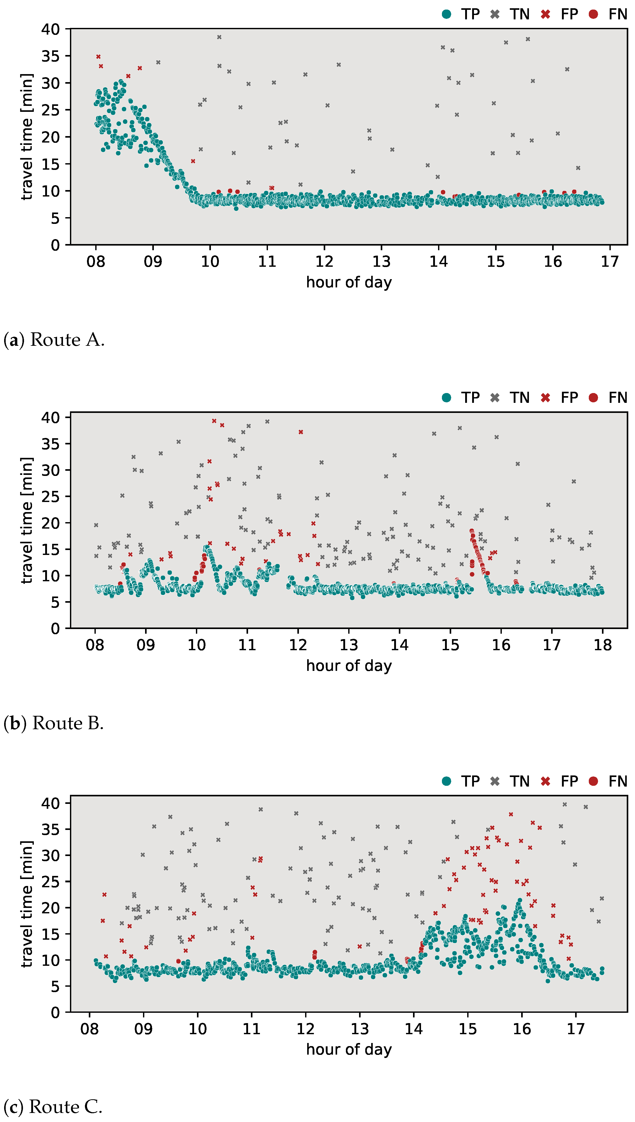
Figure 6 shows the classification results achieved using the Robinson–Polak algorithm. For route A (Figure 6a), the algorithm yielded an -score of 0.854, with a result of 0 detected FNs and 123 FPs. This represents the lowest -score among all algorithms tested on route A, indicating challenges, particularly during morning periods, when travel times gradually decrease. However, on route B (Figure 6b), the algorithm exhibited a notably high -score of 0.923, with 0 FPs and 97 FNs, suggesting minimal difficulties in adapting to abrupt changes in travel time behavior for this route configuration. When applied to route C (Figure 6c), the algorithm achieved an -score of 0.905, detecting 2 FPs and 165 FNs. In particular, the algorithm encountered challenges in classifying travel time observations during the afternoon rush hour, particularly when multiple observations of vehicles using alternative routes occurred.
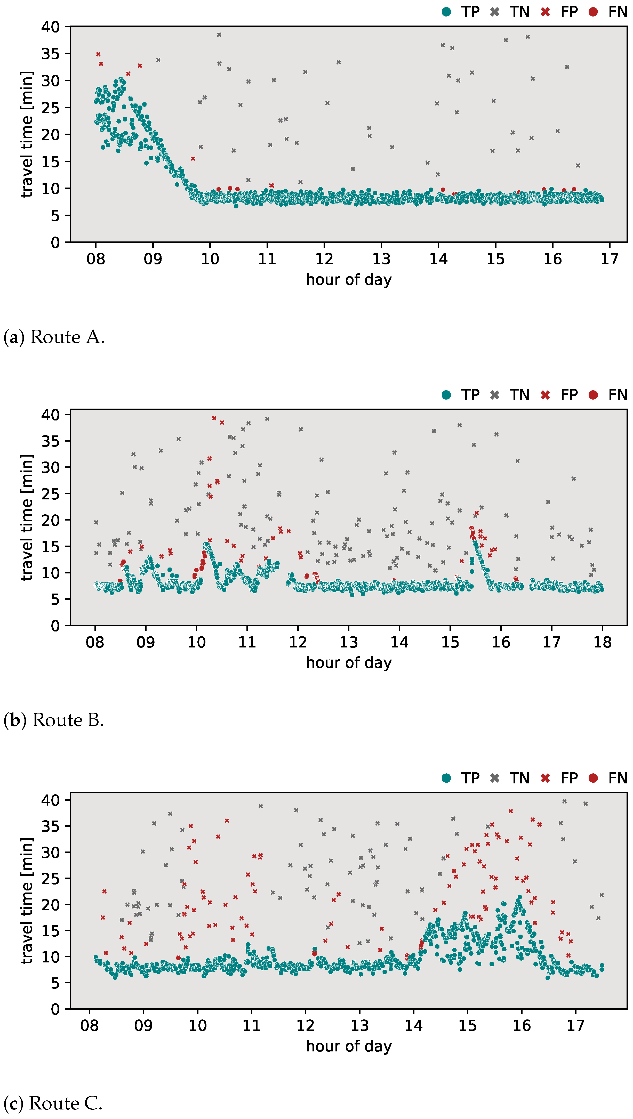
Figure 7 shows the classification results obtained using the proposed algorithm. When applied to route A (Figure 7a), the algorithm performed with an -score of 0.982, with a result of one detected FN and three FPs. For route B (Figure 7b), the algorithm exhibited an -score of 0.968, with nine FPs and one FN. For route C (Figure 7c), the algorithm achieved an -score of 0.987, with five FPs and one FN. The proposed algorithm performed with the highest -score among all tested algorithms on all routes.
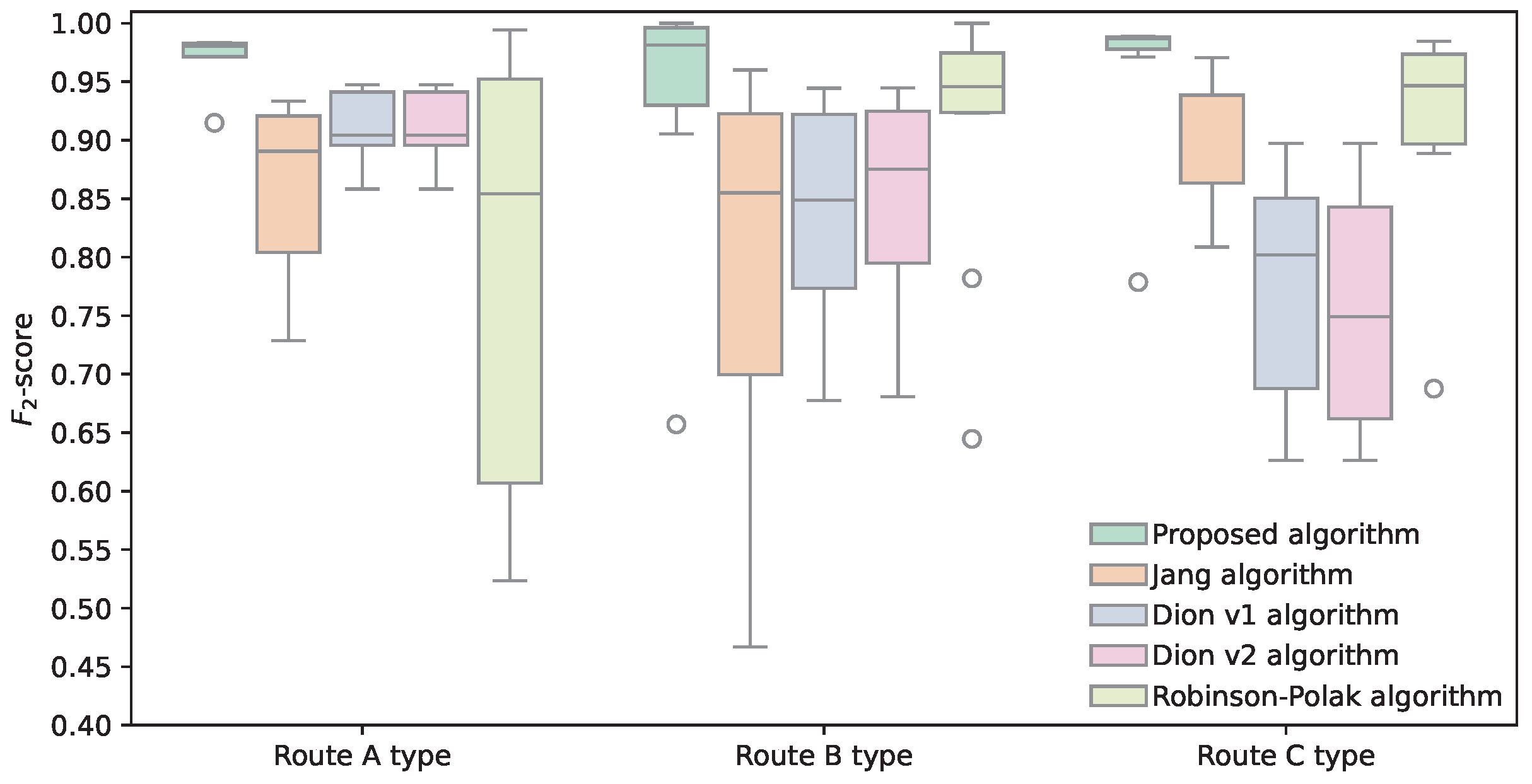
Figure 8 shows the spread of the -score metrics applied to all routes in the initial data set using box plots. It can be seen that the proposed algorithm has a consistently high -score on all types of routes. The Jang algorithm and the Dion–Rakha v1 and v2 algorithms display lower -scores with higher variability on the selected routes; however, the Dion–Rakha v1 and v2 algorithms did not perform optimally on the route C type. It can be seen that the Robinson–Polak algorithm coped well with the route B and C types, as opposed to highly variable results in the route A types.
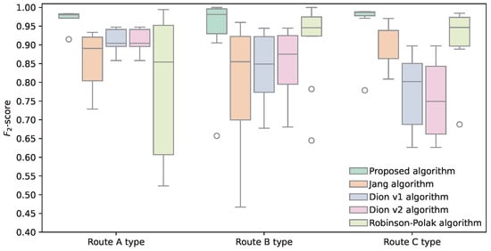
Figure 8.
Comparison of used methods’ -scores across different route types.
5. Discussion
The proposed transit traffic filtration algorithm represents a significant advancement in the accurate identification of transit traffic from matched license plate data. Unlike previous methods, which often require extensive manual calibration and are prone to misclassifying valid travel times as outliers, our algorithm introduces a dynamic, interval-based analysis. This allows for a more adaptive approach to differentiating between transit and non-transit traffic, even in complex urban environments where traffic patterns can be highly variable.
The key innovation of this algorithm lies in its iterative evaluation of travel times across consecutive intervals, which reduces the reliance on static assumptions about traffic behavior. By focusing on the temporal relationships between adjacent intervals, the algorithm effectively filters out travel times that deviate from the expected pattern, which typically indicates non-transit behavior. This is particularly important in urban settings where the variability in travel times is pronounced and traditional methods may struggle to maintain accuracy.
The proposed algorithm has demonstrated high efficiency in all predefined objectives. Through evaluation against selected algorithms, the proposed approach has shown superior -score metrics, consistently outperforming existing methods across a variety of test scenarios, including urban arterial routes, suburban commutes, and urban transit routes. The high -scores achieved across these scenarios highlight the robustness of the algorithm in correctly classifying transit traffic, minimizing both false positives and false negatives. This accuracy is crucial for traffic management applications, where the precise identification of transit traffic can inform better planning and decision making.
However, certain limitations of the current algorithm must be acknowledged. The algorithm’s reliance on time interval-based analysis may also limit its scalability across different geographic regions or traffic scenarios. Different regions may exhibit unique traffic patterns that are not easily captured by a uniform algorithm, suggesting the need for region-specific calibrations or adjustments. Although the proposed algorithm reduces the need for manual calibration compared to existing methods, it may still require some level of customization to ensure optimal performance in diverse settings.
Another notable limitation is the number of travel time records within each evaluated time interval. When the number of records is low, the reliability of the statistical analysis performed by the algorithm may be compromised, potentially leading to inaccuracies in the identification of transit traffic. The impact of this limitation will be further researched to determine how it influences the overall performance of the algorithm and to explore potential solutions, such as adaptive interval sizing or the integration of additional data sources to increase record density.
6. Conclusions
In conclusion, the transit traffic filtration algorithm introduced in this study represents a significant step forward in the accurate identification and filtering of transit traffic within complex traffic environments. By minimizing the need for extensive manual calibration and providing a more adaptive and robust solution, the algorithm offers a practical tool for traffic engineers and urban planners seeking to improve traffic management and planning. The high levels of the -score metric demonstrated in various types of routes indicate the potential for this algorithm to be widely adopted in different urban and suburban contexts.
Through a comprehensive review of the literature, suitable algorithms for the validation process were identified: Jang algorithm, Dion–Rakha versions 1 and 2, and Robinson–Polak algorithm—each exhibiting distinct strengths and limitations in managing various traffic scenarios. Closer analysis has shown that current algorithms rely largely on parameter settings for calibration and therefore pose substantial obstacles to optimal performance across various traffic scenarios and effort in the setup phase. This leads to poor elasticity of those methods and non-feasibility for automated use across different routes. In comparison, the proposed algorithm sought to simplify the classification of travel time observations without the need for extensive manual calibration and adjustments, simplifying implementation and improving usability.
Although the Jang algorithm and the Dion–Rakha algorithms primarily focus on travel time estimation tasks, which are less dependent on the correct identification of false negatives, they can potentially serve as effective tools for transit travel time filtering when appropriately calibrated. In contrast, the Robinson–Polak algorithm, designed to classify transit vehicles using the overtaking method, confronts limitations on routes characterized by significant time fluctuations or alternative routes. Moreover, its performance is intricately linked to initial parameter settings.
Furthermore, the proposed algorithm extends beyond outlier detection; its ability to filter transit vehicles with valid travel times makes it potentially suitable for travel time estimation purposes. This dual functionality improves its utility to provide reliable data to inform other traffic users. Such promising results not only validate the effectiveness of our approach but also underscore its potential to significantly advance automated outlier detection methodologies in transportation research, while simultaneously offering added value as a travel time estimation tool. In this place, it is worth highlighting that transit traffic identification (filtration) is a task different from true travel time estimation, as lower outliers are tolerated in transit filtration, whereas they are not in travel time estimation.
The proposed algorithm presents a valuable tool to improve the accuracy and efficiency of the identification of transit traffic. However, its full potential can only be realized through continued refinement and validation in diverse real-world settings. Future research should focus on addressing the identified limitations, with the goal of developing a truly universal algorithm that can be seamlessly applied across a wide range of traffic environments. Such advancements would not only enhance the utility of the algorithm for traffic engineers and urban planners but also contribute to the broader goal of creating more efficient, sustainable, and resilient transportation systems.
By continuing to refine the proposed method and exploring its application in new contexts, we can move closer to achieving a comprehensive solution for transit traffic filtration. This ongoing work will be crucial in ensuring that the algorithm remains at the forefront of traffic data analysis and continues to provide valuable insights to improve urban mobility and reduce the environmental impact of transportation systems.
Author Contributions
Conceptualization, P.R.; methodology, P.R. and M.M.; software, P.R.; validation, P.R.; formal analysis, P.R.; investigation, P.R.; resources, P.R. and P.K.; data curation, P.R.; writing—original draft preparation, P.R.; writing—review and editing, P.R. and M.M.; visualization, P.R.; supervision, P.K.; project administration, P.R. and P.K.; funding acquisition, M.M. All authors have read and agreed to the published version of the manuscript.
Funding
This research received no external funding.
Institutional Review Board Statement
Not applicable.
Informed Consent Statement
Not applicable.
Data Availability Statement
The data presented in this study are available on request from the corresponding author.
Conflicts of Interest
The authors declare no conflicts of interest.
References
- Qi, W.; Rao, B.; Fu, C. A Novel Filtering Method of Travel-Time Outliers Extracted from Large-Scale Traffic Checkpoint Data. J. Transp. Eng. Part Syst. 2024, 150. [Google Scholar] [CrossRef]
- Nadrian, H.; Heizomi, H.; Shirzadi, S.; Moradi, M.S.; Hajibadali, P. Exploring the dimensions of urban quality of life associated with urban traffic jam: The development and validation of an instrument. J. Transp. Health 2022, 26, 101463. [Google Scholar] [CrossRef]
- Cats, O.; West, J.; Eliasson, J. A dynamic stochastic model for evaluating congestion and crowding effects in transit systems. Transp. Res. Part Methodol. 2016, 89, 43–57. [Google Scholar] [CrossRef]
- Fowkes, A.S. The Use of Number Plate Matching For Vehicle Travel Time Estimation. In Proceedings of the Seminar, Developing Countries, the PTRC Annual Summer Meeting, University of Warwick, Coventry, UK, 4–7 July 1983; p. 240. [Google Scholar]
- Montgomery, F.; May, A. Fators Affecting Travel Times on Urban Radial Routes. Traffic Eng. Control 1987, 28, 452–458. [Google Scholar]
- Clark, S.D.; Grant-Muller, S.; Chen, H. Cleaning of Matched License Plate Data. Transp. Res. Rec. 2002, 1804, 1–7. [Google Scholar] [CrossRef]
- Robinson, S.; Polak, J. Overtaking rule method for the cleaning of matched license-plate data. J. Transp. Eng. 2006, 132, 609–617. [Google Scholar] [CrossRef]
- Dion, F.; Rakha, H. Estimating dynamic roadway travel times using automatic vehicle identification data for low sampling rates. Transp. Res. Part Methodol. 2006, 40, 745–766. [Google Scholar] [CrossRef]
- Houston TranStar—About Houston TranStar. Available online: https://www.houstontranstar.org/about_transtar/ (accessed on 15 August 2023).
- Southwest Research Institute. Automated Vehicle Identification Model Deployment Initiative System Design Document; Technical Report SwRI Project No. 10-8684; Southwest Research Institute: San Antonio, TX, USA, 1998. [Google Scholar]
- Mouskos, K.C.; Niver, E.; Pignataro, L.J.; Lee, S.W.; Antoniou, N.; Papadoupolos, L. Transmit System Evaluation; Final Report; New Jersey Institute of Technology: Newark, NJ, USA, 1998. [Google Scholar]
- Zheng, P.; McDonald, M. Estimation of travel time using fuzzy clustering method. IET Intell. Transp. Syst. 2009, 3, 77–86. [Google Scholar] [CrossRef]
- Bezdek, J.C. Pattern Recognition with Fuzzy Objective Function Algorithms; Springer US: Boston, MA, USA, 1981. [Google Scholar] [CrossRef]
- Moghaddam, S.; Hellinga, B. Algorithm for detecting outliers in Bluetooth data in real time. Transp. Res. Rec. 2014, 2442, 129–139. [Google Scholar] [CrossRef]
- Jang, J. Outlier filtering algorithm for travel time estimation using dedicated short-range communications probes on rural highways. IET Intell. Transp. Syst. 2016, 10, 453–460. [Google Scholar] [CrossRef]
- Asqool, O.; Koting, S.; Saifizul, A. Evaluation of outlier filtering algorithms for accurate travel time measurement incorporating lane-splitting situations. Sustainability 2021, 13, 3851. [Google Scholar] [CrossRef]
- Li, J.; Van Zuylen, H.; Deng, Y.; Zhou, Y. Urban travel time data cleaning and analysis for Automatic Number Plate Recognition. Transportation Res. Procedia 2020, 47, 712–719. [Google Scholar] [CrossRef]

Disclaimer/Publisher’s Note: The statements, opinions and data contained in all publications are solely those of the individual author(s) and contributor(s) and not of MDPI and/or the editor(s). MDPI and/or the editor(s) disclaim responsibility for any injury to people or property resulting from any ideas, methods, instructions or products referred to in the content. |
© 2024 by the authors. Licensee MDPI, Basel, Switzerland. This article is an open access article distributed under the terms and conditions of the Creative Commons Attribution (CC BY) license (https://creativecommons.org/licenses/by/4.0/).