
Fast Fault Line Selection Technology of Distribution Network Based on MCECA-CloFormer


Abstract
:1. Introduction
- A method based on moving average filter (MAF) and motif difference field (MDF) for converting time series into images is proposed. The method starts with a moving average denoising of the one-dimensional zero-sequence current signal and then encodes it into a two-dimensional image using the motif difference field. The color distributions in MDF images are more intuitive and contain richer information than time-series data, and the image data can also be used directly as input for deep learning-based visual models.
- A faulty line selection model based on MCECA-CloFormer is proposed. The line selection model utilizes the MCECA module to fuse fault images from multiple measurement points and the CloFormer module with a two-branch structure to sense the difference between fault and non-fault feature maps. It has been demonstrated that the model can achieve fast and accurate fault line selection in target distribution networks under different operating conditions and line parameters.
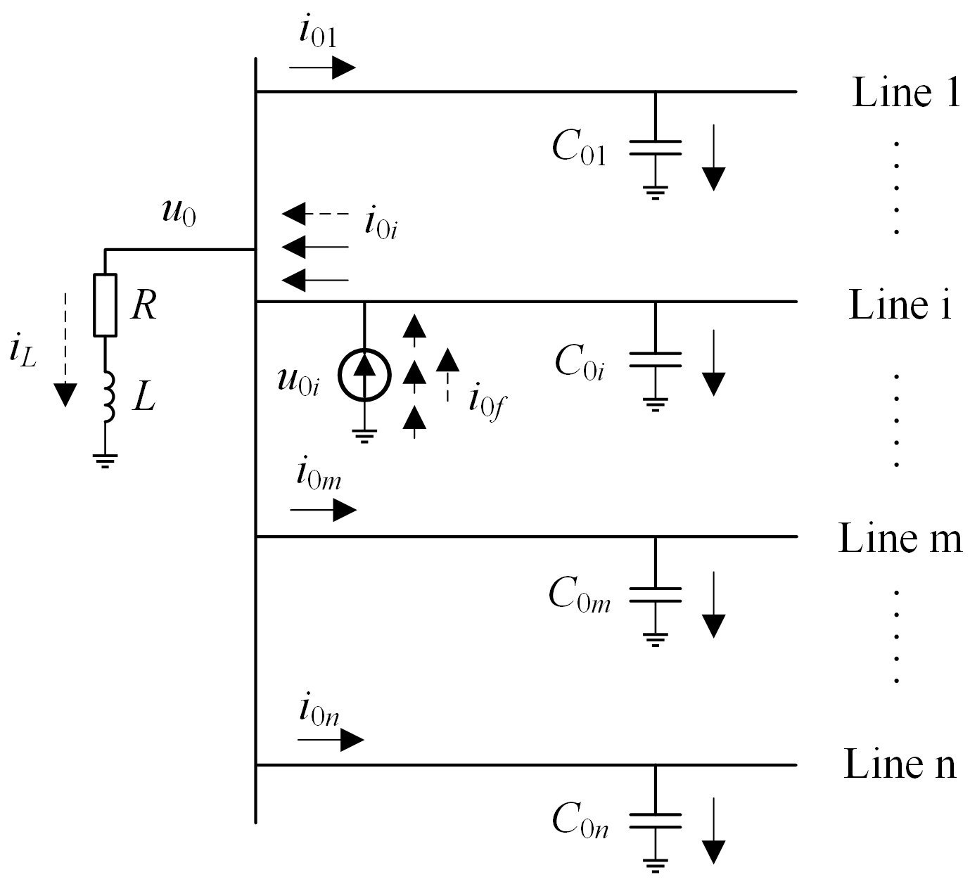
2. Characteristics Analysis of Single-Phase Grounding Fault
3. Imaging Method Based on MAF-MDF
3.1. Moving Average Filter
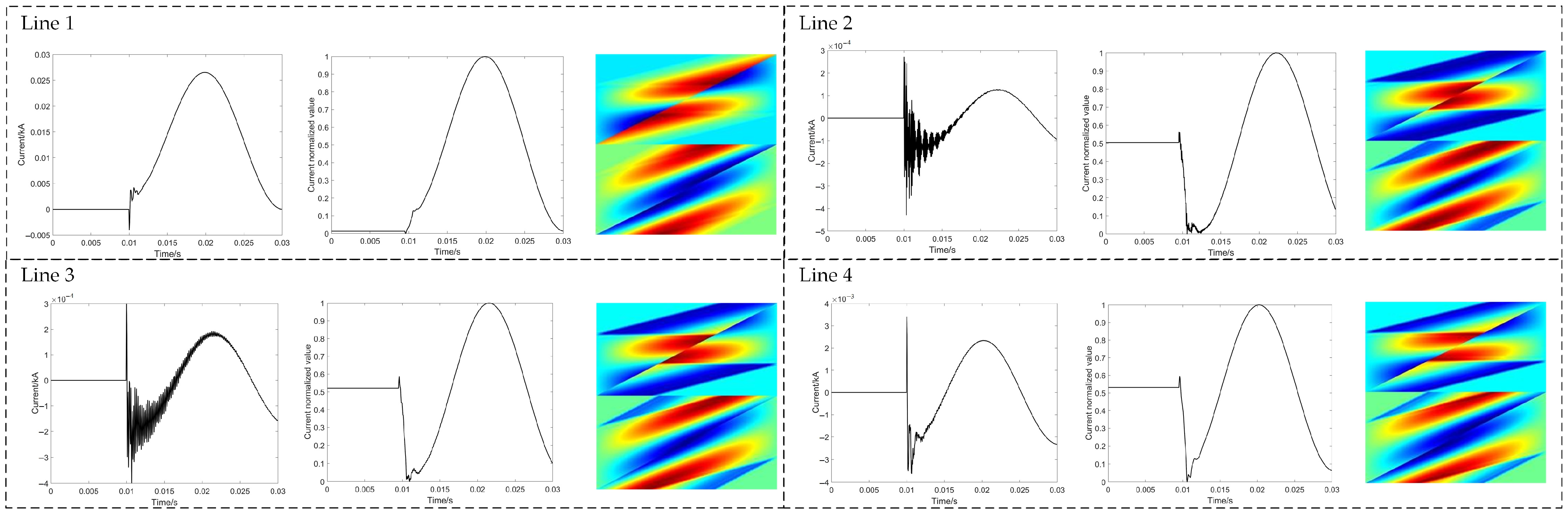
3.2. Motif Difference Field
3.3. MAF-MDF
4. Fault Line Selection Model Based on MCECA-CloFormer
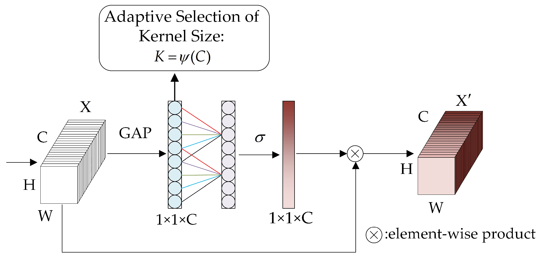
4.1. Efficient Channel Attention
4.2. CloFormer
- Conv stem. This component primarily comprises five convolutional layers, with the detailed structure illustrated in Figure 5a.
- Clo block. This part is constituted by a local branch and a global branch. As shown in Figure 5b, within the global branch, K and V are initially downsampled, followed by the execution of a standard attention process on Q, K, and V to extract global low-frequency information, as outlined in Equation (15).
- ConvFFN. This component primarily bolsters its local information aggregation capacity by introducing depthwise convolution following the GELU activation function. Two modes are adopted: one without downsampling (depicted on the left in Figure 5c), which is utilized in all layers except the last, and another incorporating a downsampling module (shown on the right in Figure 5c), which is employed in the final layer of the CloFormer architecture.
- Output module. The output module consists of a global average pooling layer and a linear classifier. The overall structure of CloFormer is depicted in Figure 5d, wherein a CloLayer is composed of a combination of two Clo blocks and a ConvFFN, with downsampling incorporated in the ConvFFN of the final layer.
4.3. MCECA-CloFormer
4.4. Implementation Flow of Line Selection Method
5. Simulation Results and Discussion
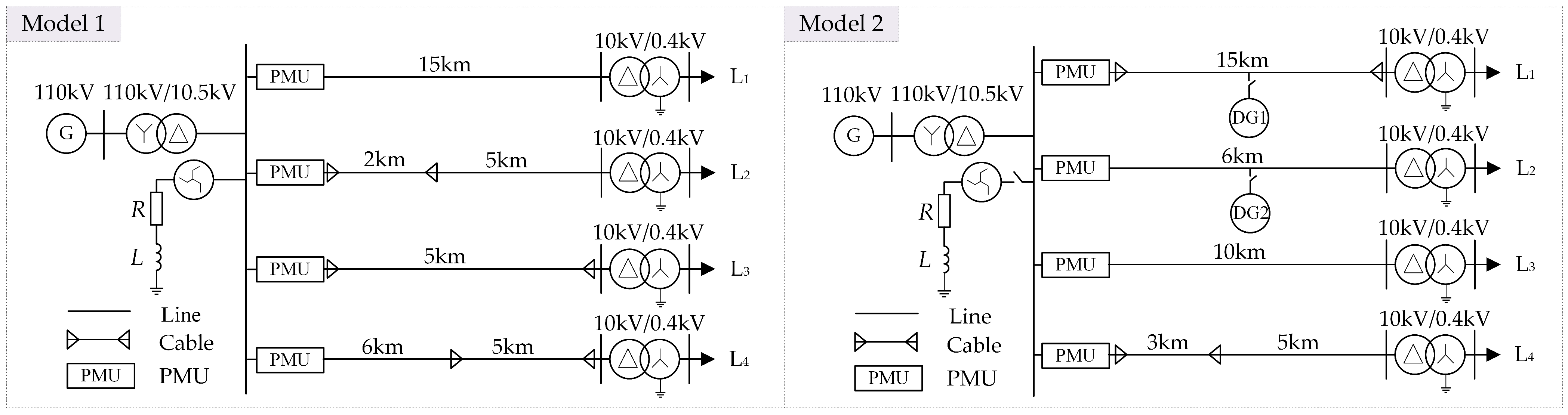
5.1. Dataset
5.2. Training and Testing of the Model
5.3. Noise Resistance Test and Algorithm Comparison Analysis
5.4. The Impact of Missing Data on Algorithm Performance
5.5. Analysis and Testing of Actual Waveform Recordings
5.6. Discussion
6. Conclusions and Future Work
Author Contributions
Funding
Data Availability Statement
Conflicts of Interest
References
- Hao, S.; Zhang, X.; Ma, R.; Wen, H.; Ma, X.; An, B.; Li, J. Fault Line Selection Method for Small Current Grounding System Based on Improved GoogLeNet. Power Syst. Technol. 2022, 46, 361–368. [Google Scholar] [CrossRef]
- Wei, X.; Yang, D. An Adaptive Fault Line Selection Method Based on Wavelet Packet Comprehensive Singular Value for Small Current Grounding System. In Proceedings of the 2015 5th International Conference on Electric Utility Deregulation and Restructuring and Power Technologies (DRPT), Changsha, China, 26–29 November 2015; IEEE: New York, NY, USA; pp. 1110–1114. [Google Scholar]
- Hao, Q.; Tianyou, L. High Impedance Fault Line Selection Method for Resonant Grounding System Based on Wavelet Packet Analysis. In Proceedings of the 2018 China International Conference on Electricity Distribution (CICED), Tianjin, China, 17–19 September 2018; IEEE: New York, NY, USA; pp. 1174–1179. [Google Scholar]
- Song, J.; Li, Y.; Zhang, Y. Faulty Line Detection Method Based on Improved Hilbert-Huang Transform for Resonant Grounding Systems. Int. Trans. Electr. Energ. Syst. 2021, 31, e12760. [Google Scholar] [CrossRef]
- Cao, W.; Li, C.; Li, Z.; Wang, S.; Pang, H. Research on Low-Resistance Grounding Fault Line Selection Based on VMD with PE and K-Means Clustering Algorithm. Math. Probl. Eng. 2022, 2022, 5360302. [Google Scholar] [CrossRef]
- Chen, B.; Sun, Y.; Song, X.; Wang, B. Regionalized Fault Line in Distribution Networks Based on an Improved SSA-VMD and Multi-Scale Fuzzy Entropy. Electr. Eng. 2023, 105, 4399–4408. [Google Scholar] [CrossRef]
- Gong, J. Wavelet Packet Coefficient of Transient First Half Wave Line Selection Method for Single-Phase Grounding Fault. IOP Conf. Ser. Earth Environ. Sci. 2022, 983, 012012. [Google Scholar] [CrossRef]
- Hou, S.; Guo, W. Optimal Denoising and Feature Extraction Methods Using Modified CEEMD Combined with Duffing System and Their Applications in Fault Line Selection of Non-Solid-Earthed Network. Symmetry 2020, 12, 536. [Google Scholar] [CrossRef]
- Li, J.; Yan, J.; Huang, L. Research on Fault Line Selection Algorithm for Economic Operation of Power Grids Based on Improved Variational Modal Decomposition. In Proceedings of the 2023 International Conference on Advances in Electrical Engineering and Computer Applications (AEECA), Dalian, China, 18 August 2023; IEEE: New York, NY, USA; pp. 6–11. [Google Scholar]
- Li, Z.; Li, W.; Peng, W.; Lei, L.; Liang, L. Single-phase-to-ground Fault Line Selection Method of Distribution Network Based on IHHT-RF. J. Electr. Power Sci. Technol. 2024, 39, 171–182. [Google Scholar] [CrossRef]
- Liu, Y.; Liu, X.; Fan, S.; Ma, X.; Deng, S. Single-Phase-to-Ground Fault Line Selection Method Based on STOA-SVM. J. Phys. Conf. Ser. 2021, 2095, 012029. [Google Scholar] [CrossRef]
- Wang, F.; Zhang, Z.; Wu, K.; Jian, D.; Chen, Q.; Zhang, C.; Dong, Y.; He, X.; Dong, L. Artificial Intelligence Techniques for Ground Fault Line Selection in Power Systems: State-of-the-Art and Research Challenges. Math. Biosci. Eng. 2023, 20, 14518–14549. [Google Scholar] [CrossRef]
- Guo, M.-F.; Gao, J.-H.; Shao, X.; Chen, D.-Y. Location of Single-Line-to-Ground Fault Using 1-D Convolutional Neural Network and Waveform Concatenation in Resonant Grounding Distribution Systems. IEEE Trans. Instrum. Meas. 2021, 70, 1–9. [Google Scholar] [CrossRef]
- Wang, N. Fault Line Selection of Power Distribution System via Improved Bee Colony Algorithm Based Deep Neural Network. Energy Rep. 2022, 8, 43–53. [Google Scholar] [CrossRef]
- Cheng, X.-R.; Cui, B.-J.; Hou, S.-Z. Fault Line Selection of Distribution Network Based on Modified CEEMDAN and GoogLeNet Neural Network. IEEE Sens. J. 2022, 22, 13346–13364. [Google Scholar] [CrossRef]
- Anbarasi, A.; Nithyasree, K.C. Nithyasree COVID-19 Detection in CT Images Using Deep Transfer Learning. Int. Trans. Electr. Eng. Comput. Sci. 2022, 1, 1–7. [Google Scholar] [CrossRef]
- Mahmoud, K.A.A.; Badr, M.M.; Elmalhy, N.A.; Hamdy, R.A.; Ahmed, S.; Mordi, A.A. Transfer Learning by Fine-Tuning Pre-Trained Convolutional Neural Network Architectures for Switchgear Fault Detection Using Thermal Imaging. Alex. Eng. J. 2024, 103, 327–342. [Google Scholar] [CrossRef]
- Hu, J.; Chen, M.; Tang, H.; Zhang, J. An Adversarial Transfer Learning Method Based on Domain Distribution Prediction for Aero-Engine Fault Diagnosis. Eng. Appl. Artif. Intell. 2024, 133, 108287. [Google Scholar] [CrossRef]
- Liu, C.; Wang, X.; Shang, B.; Luo, G.; Liu, Z. Fault Line Selection for Active Distribution Network Based on Domain Adaptive Transfer Learning. High Volt. Eng. 2024, 50, 3050–3059. [Google Scholar] [CrossRef]
- Su, X.; Wei, H. A Fault-Line Selection Method for Small-Current Grounded System Based on Deep Transfer Learning. Energies 2022, 15, 3467. [Google Scholar] [CrossRef]
- Guo, L.; Qu, X.; Wang, X.; Wang, Y.; Tian, Y.; Zhang, F. A Novel Fault Feeder Selection Method for Resonant Grounding Distribution Networks Based on Improved Hough Transform. Electric Power. 2024, 57, 132–142. [Google Scholar]
- Zhang, Y.; Gan, F.; Chen, X. Motif Difference Field: An Effective Image-Based Time Series Classification and Applications in Machine Malfunction Detection. In Proceedings of the 2020 IEEE 4th Conference on Energy Internet and Energy System Integration (EI2), Wuhan, China, 30 October 2020; IEEE: New York, NY, USA; pp. 3079–3083. [Google Scholar]
- Wang, Q.; Wu, B.; Zhu, P.; Li, P.; Zuo, W.; Hu, Q. ECA-Net: Efficient Channel Attention for Deep Convolutional Neural Networks. In Proceedings of the 2020 IEEE/CVF Conference on Computer Vision and Pattern Recognition (CVPR), Seattle, WA, USA, 13–19 June 2020; IEEE: New York, NY, USA; pp. 11531–11539. [Google Scholar]
- Fan, Q.; Huang, H.; Guan, J.; He, R. Rethinking Local Perception in Lightweight Vision Transformer. arXiv 2023, arXiv:2303.17803. [Google Scholar]
- Gautam, S. Brahma Detection of High Impedance Fault in Power Distribution Systems Using Mathematical Morphology. IEEE Trans. Power Syst. 2013, 28, 1226–1234. [Google Scholar] [CrossRef]
- Jiang, W.; Wu, Z.; Li, W.; She, Y.; Hu, Y. Control Strategy of Suppressing Negative Sequence Current of Grid-Connected Inverter Base on Asymmetric Grid. Trans. China Electrotech. Soc. 2015, 30, 77–84. [Google Scholar] [CrossRef]


| Algorithm | Parameters |
|---|---|
| MAF | Window width = 19 |
| MDF | n = 3 |
| ECA | γ = 2; b =1 |
| CloFormer | Channels: [32, 64, 128, 256]; Heads: [4, 4, 8, 16]; Kernel Size: [3, 5, 7, 9] |
| Type | Sequence | Resistance/(Ω/km) | Inductance/(mH/km) | Capacitance/(μF/km) |
|---|---|---|---|---|
| Line | positive | 0.1273 | 0.9337 | 0.0127 |
| zero | 0.3864 | 4.1264 | 0.0078 | |
| Cable | positive | 0.2650 | 0.2550 | 0.1700 |
| zero | 2.5400 | 1.1019 | 0.1530 |
| Type | Sequence | Resistance/(Ω/km) | Inductance/(mH/km) | Capacitance/(μF/km) |
|---|---|---|---|---|
| Line | positive | 0.1700 | 1.0170 | 0.1150 |
| zero | 0.3200 | 3.5600 | 0.0060 | |
| Cable | positive | 0.2700 | 0.2550 | 0.3760 |
| zero | 2.7000 | 1.1090 | 0.2760 |
| Type | Parameter |
|---|---|
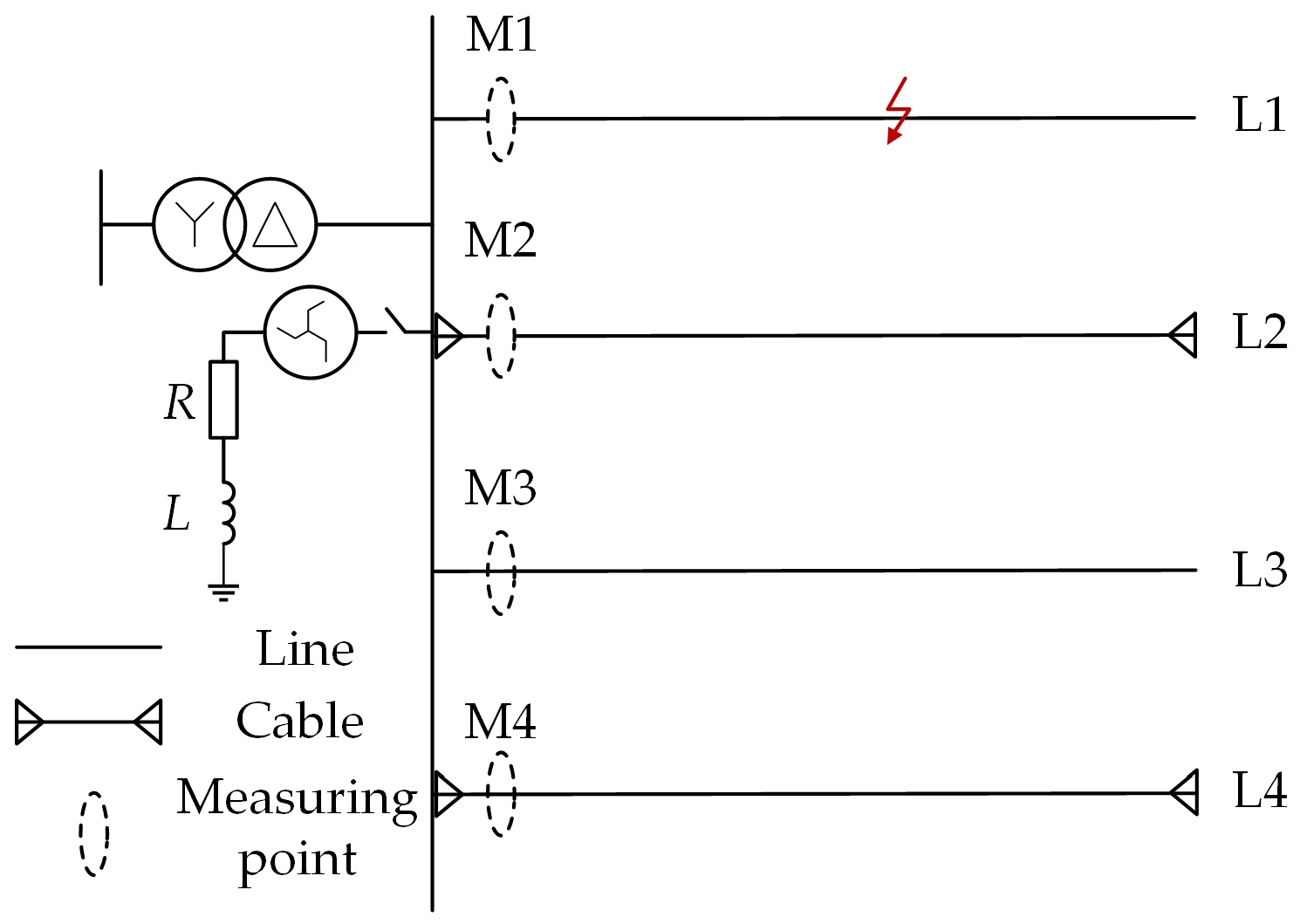
| faulty line | L1, L2, L3, L4 |
| fault location | 10%, 20%, 30%, 40%, 50%, 60%, 70%, 80%, 90% |
| fault ground resistance | 0.1 Ω, 1 Ω, 10 Ω, 100 Ω, 1000 Ω, 3000 Ω, 5000 Ω, Emanuel |
| initial fault phase angle | 0°, 30°, 60°, 90°, 120°, 150°, 180° |
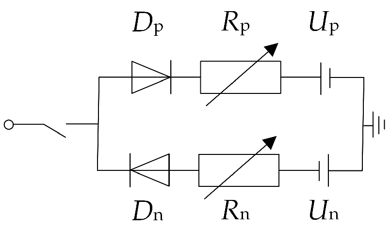
| Model | Up/kV | Un/kV | Rp/Ω | Rn/Ω |
|---|---|---|---|---|
| HIF 1 | 2 | 3 | 350 | 350 |
| HIF 2 | 1.3 | 1.6 | 450 | 450 |
| HIF 3 | 2.4 | 3.4 | 650 | 650 |
| Type | Faulty Line | Fault Location | Fault Ground Resistance | Initial Fault Phase Angle | Test Content |
|---|---|---|---|---|---|
| parameter | L1, L2, L3, L4 | 15%, 35%, 75% | 10 Ω | 0° | Effect of fault location |
| 50% | 2 Ω, 200 Ω, 4000 Ω | 0° | Effect of fault ground resistance | ||
| 50% | 10 Ω | 20°, 45°, 160° | Effect of Initial fault phase angle |
| Model | SNR = 40 dB | SNR = 30 dB | SNR = 20 dB | SNR = 10 dB |
|---|---|---|---|---|
| MCECA-CloFormer | 100% | 100% | 100% | 99.33% |
| MCloFormer-ECA | 100% | 100% | 99.67% | 98.33% |
| MCNN-CloFormer | 99.00% | 99.00% | 99.00% | 98.33% |
| MCECA-MobileNetV2 | 98.00% | 97.67% | 98.00% | 96.33% |
| MCECA-ECANet | 100% | 100% | 100% | 99.01% |
| Model | Time |
|---|---|
| MCECA-CloFormer | 0.0420 s |
| MCloFormer-ECA | 0.1290 s |
| MCNN-CloFormer | 0.0350 s |
| MCECA-MobileNetV2 | 0.0220 s |
| MCECA-ECANet | 0.1800 s |
| Data Missing Rate | Accuracy |
|---|---|
| 5% | 99.67% |
| 10% | 100% |
| 20% | 99.00% |
| 30% | 94.68% |
Disclaimer/Publisher’s Note: The statements, opinions and data contained in all publications are solely those of the individual author(s) and contributor(s) and not of MDPI and/or the editor(s). MDPI and/or the editor(s) disclaim responsibility for any injury to people or property resulting from any ideas, methods, instructions or products referred to in the content. |
© 2024 by the authors. Licensee MDPI, Basel, Switzerland. This article is an open access article distributed under the terms and conditions of the Creative Commons Attribution (CC BY) license (https://creativecommons.org/licenses/by/4.0/).
Share and Cite
Ding, C.; Ma, P.; Jiang, C.; Wang, F. Fast Fault Line Selection Technology of Distribution Network Based on MCECA-CloFormer. Appl. Sci. 2024, 14, 8270. https://doi.org/10.3390/app14188270
Ding C, Ma P, Jiang C, Wang F. Fast Fault Line Selection Technology of Distribution Network Based on MCECA-CloFormer. Applied Sciences. 2024; 14(18):8270. https://doi.org/10.3390/app14188270
Chicago/Turabian StyleDing, Can, Pengcheng Ma, Changhua Jiang, and Fei Wang. 2024. "Fast Fault Line Selection Technology of Distribution Network Based on MCECA-CloFormer" Applied Sciences 14, no. 18: 8270. https://doi.org/10.3390/app14188270