Numerical Simulation of Seismic-Wave Propagation in Specific Layered Geological Structures

Abstract

This study presents a numerical simulation approach used to investigate seismic-wave propagation in specific geological structures. Using the LS-DYNA software, the simulation incorporated a TNT explosion model to simulate seismic energy released during earthquakes. It provides a new method to investigate the propagation characteristics of seismic-waves within geological structures. Firstly, the measurement conditions and geological settings of the seismic event on 18 February 2012 in Northeast China are presented. Subsequently, a numerical simulation model of seismic-wave propagation is developed. The simulation result validates it by comparing it with recorded data from seismic stations, demonstrating a promising correspondence between the simulated and observed data. Additionally, the simulation simulates the seismic-wave propagation within water and layered geological structures, validating the numerical simulation model. The numerical model is an effective tool for simulating the propagation of seismic waves in geological structures. This study is important for evaluating seismic-wave propagation using the simulation method.

1. Introduction

The propagation of seismic waves through geological structures represents a pivotal area of investigation in the comprehension and mitigation of seismic activity [1,2]. Seismic-wave propagation correlates with geophysical structures [3,4]. Analyzing stress-wave propagation is crucial in understanding mechanical properties [5,6]. One of the most prevalent methodologies in the field of seismic-wave studies is the inversion of seismic waves [7,8,9]. This technique functions in a manner analogous to a geophysical X-ray, utilizing data derived from the Earth’s surface to construct a comprehensive image of the underlying geological structures [10,11]. Seismic-wave inversion has become a standard practice in the oil and gas industry for mapping the subterranean terrain, due to its high degree of accuracy [7,12,13].

In the field of seismic-wave inversion, numerical simulations have become an indispensable tool for advancing scientific understanding [14,15,16]. The simulations of seismic-wave propagation within the Earth provide an exemplar of the potential for earthquake-induced seismic activity, quantifying probable surface disruptions [17,18,19]. The incorporation of parameters that accurately reflect the characteristics of the medium of the Earth into seismic-wave simulations has the potential to enhance our theoretical understanding of these phenomena [14,20]. These simulations are not just tools; they provide insight into the propagation of seismic waves, thereby improving the accuracy of seismic-wave inversion techniques [21,22]. Notwithstanding the considerable advances made in the comprehension of seismic-wave behavior through numerical simulations, there has been a paucity of studies that have investigated the propagation of seismic waves from the source.

LS-DYNA is a finite-element analysis software widely used in the engineering sciences [23]. LS-DYNA software has a diverse range of applications in the simulation of explosive shock wave generation and propagation, as well as in the analysis of the dynamic response of materials [24]. The software has been utilized for the assessment of overpressure in steel tunnels subjected to external explosions and the modeling of shock wave effects [25,26]. Furthermore, LS-DYNA has effectively captured the intricate interactions between shock and explosion waves and surrounding structures [27]. This is exemplified in the analysis of gas explosions within confined roadways and challenging geological settings [28]. Nevertheless, there is a paucity of LS-DYNA simulations of seismic-wave generation and propagation.

This study introduces a new numerical simulation method for the study of seismic-wave propagation in geological structures. The energy released during these simulations is considered to be equivalent to that of a TNT explosion. For the first time, the TNT energy release process is used to simulate the generation of seismic waves during earthquakes, which is an innovation in our research approach. Furthermore, the simulated results are compared with actual seismic data from the 2012 Northeast China earthquake, verifying the model’s effectiveness in predicting seismic-wave propagation in geological structures. To verify the model’s applicability in various geological conditions, the simulation model is used to simulate seismic-wave propagation and stress distribution features in different geological settings, including water and layered geological structures. Subsequently, an equivalent blast response numerical simulation methodology is put forth for the examination of stress-wave propagation within a particular geological structure.

The paper is structured as follows: Section 2 presents a seismic event condition located in northeast China. Section 3 presents a numerical simulation model and the simulation result of seismic-wave propagation in a geological structure. Section 4 presents the methodological extensions, with a particular focus on the explosion response in water and layered geological media. Section 5 presents the conclusions of this study.

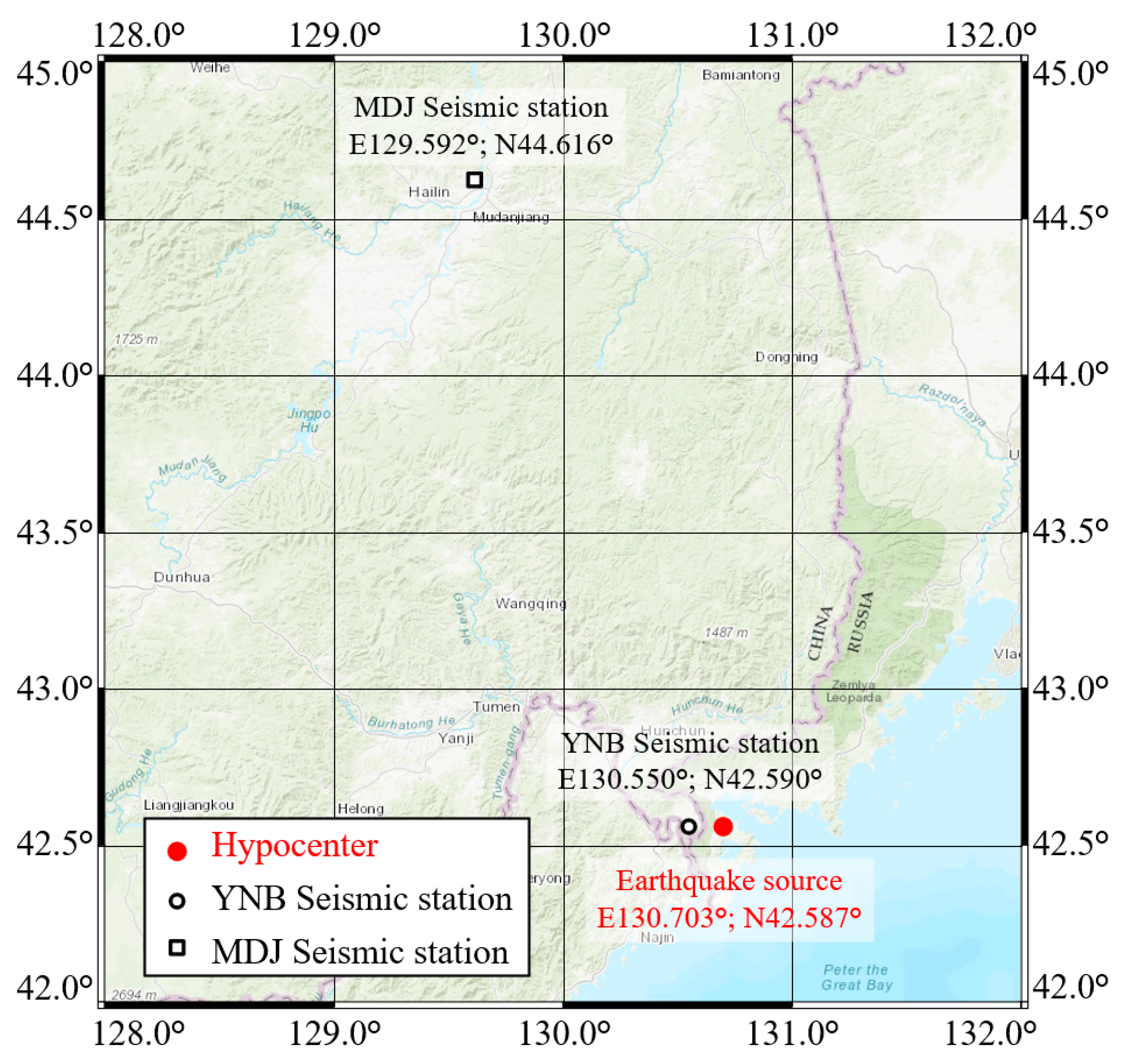
2. Seismic Event Conditions

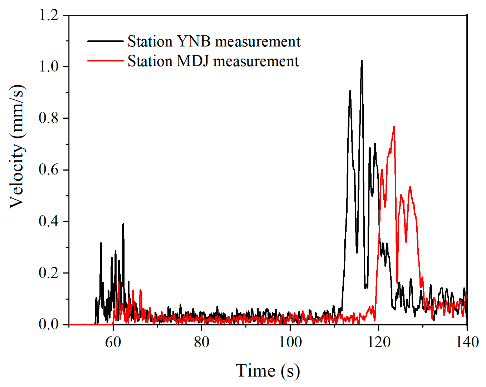
2.1. Measurement Conditions

In this study, a numerical simulation method utilizing the ANSYS LS-DYNA 970 software is employed to analyze a specific seismic event that occurred on 18 February 2012. This event serves as a practical case study, analyzing the dynamics of seismic-wave propagation through geological structures. This analysis confirms the accuracy of the simulation’s methods. The seismic event with the epicenter shown in Figure 1 was recorded at the coordinates 130.703° E longitude and 42.587° N latitude. This seismic event, measured at a focal depth of 578 km and a moment magnitude of 6.9, was recorded using data processed from measurements at the Yanbian (YNB) and Mudanjiang (MDJ) seismic stations. The YNB seismic station, located at 130.550° E longitude and 42.590° N latitude, is approximately 12 km from the epicenter and directly above the hypocenter, which is at a depth of 578 km. The station is constructed on a granite base. The MDJ seismic station is situated at 129.592° E longitude and 44.616° N latitude, approximately 242 km from the hypocenter. The amplitudes of the velocities recorded at the YNB and MDJ seismic stations, representing the combined velocities of seismic waves traveling in three directions, are directly measured and presented as resultant velocities in Figure 2. As depicted in Figure 2, at the YNB seismic station, the velocity reaches a peak of 1.025 mm/s at 116 s after the onset of the seismic event. Meanwhile, at the MDJ seismic station, located farther from the epicenter, the velocity peaks at 0.768 mm/s at 123 s following the onset of the seismic event.

By applying the Gutenberg–Richter formula, a correlation was established between the earthquake magnitude and its energy release, as described by Equation (1) [29].

$$\mathrm{l}\mathrm{g} E=aM+b,$$

(1)

where $E$ denotes the energy in J, and $M$ represents the magnitude, with the unit in Nm. For surface-wave magnitude, $a=1.5$ and $b=4.8$, whereas for moment magnitude, $a=1.5$ and $b=9.1$ [29]. It is assumed that these coefficients are sufficiently representative of the area being analyzed, despite being initially derived from global data [29].

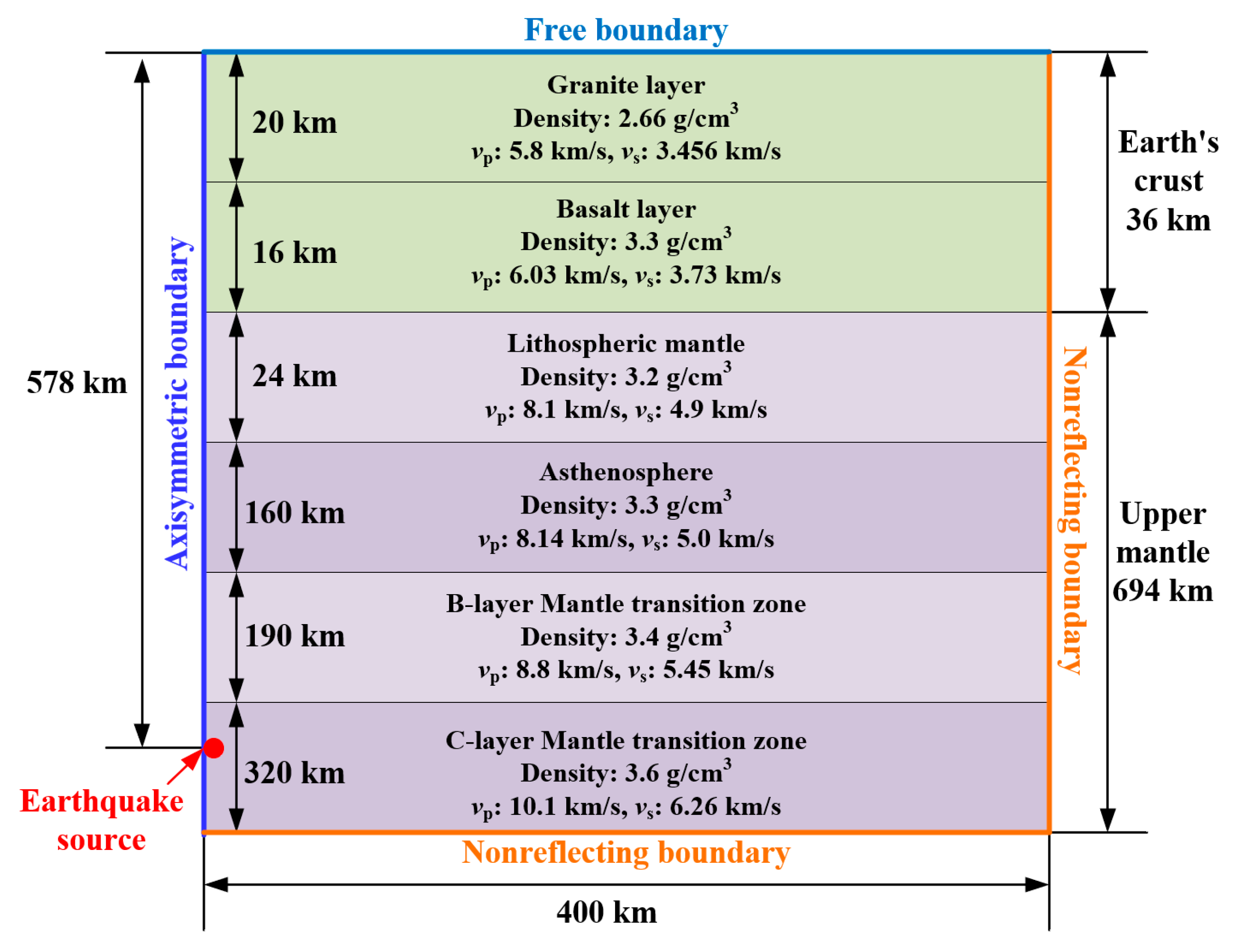
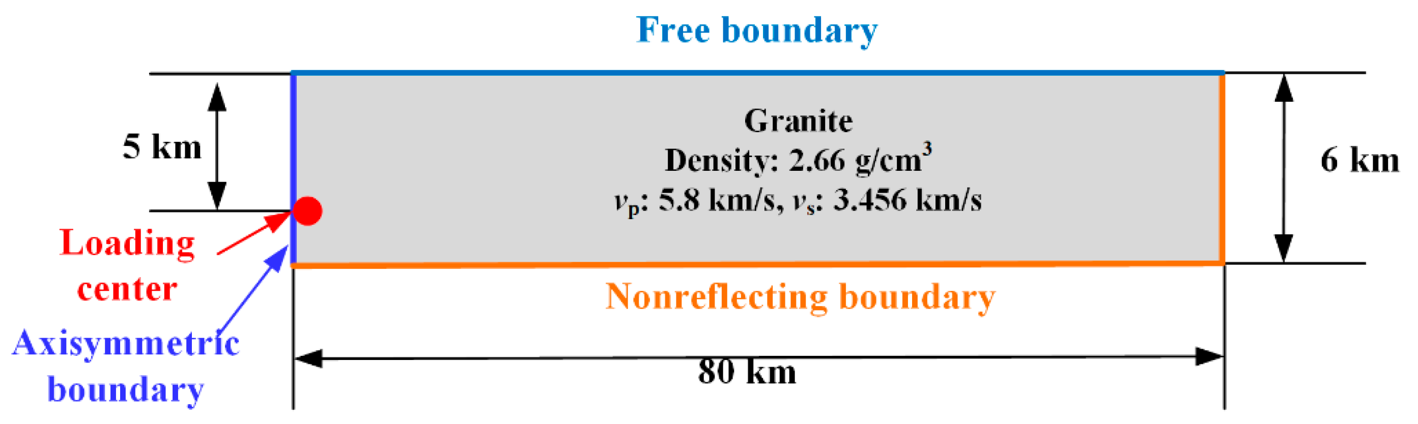
2.2. Analysis of Geological Conditions

The accuracy of a numerical simulation model in earthquake studies is often validated by comparing its results with seismic measurement data [30]. A thorough understanding of the geological parameters within the seismic zone is critical for accurately predicting seismic-wave behavior and assessing potential risk in earthquake-prone areas. This includes geological stratification and the respective density and wave velocities of each layer [31,32]. To simulate an earthquake with a focal depth of 578 km, it is necessary to consider the geological structure parameters of both the crust and the upper mantle.

The crust exhibits considerable variation in thickness, with a tendency for greater thickness in continental regions and lesser thickness in oceanic regions. Significant variations are observed across different oceans. For example, the crust is observed to be thinnest at mid-ocean ridges, such as those in the Pacific and Atlantic Oceans [33]. Discontinuities divide the crust into upper and lower layers [34]. The upper stratum is synonymous with the granite rock layer, whereas the lower stratum corresponds to the basalt rock layer [32,35]. The granite layer, mainly constituted of granite, shows minor variations in its material parameters: density (2.54–2.66 g/cm³), porosity (0.1–4.0%), tensile strength (7.00–25.00 MPa), Young’s modulus (20.0–60.0 GPa), and Poisson’s ratio (0.1–0.3). In contrast, basalt, a rock similar in chemical composition to gabbro or diabase, exhibits a wide range of parameters: density (2.70–3.30 g/cm³), porosity (0.1–1.0%), tensile strength (10.00–30.00 MPa), Young’s modulus (60.0–100.0 GPa), and Poisson’s ratio (0.1–0.35) [36].

The upper mantle encompasses the B layer (Moho surface to ~400 km) and the C layer (440 to ~960 km). Its average density ranges from 3.2 to 3.6 g/cm³. The P-wave velocities span from 8.1 to 10.1 km/s, and the S-wave velocities span from 4.4 to 6.4 km/s [37]. Predominantly formed of peridotite, the mantle has a solid rock layer which, together with the crust, forms the rigid lithosphere [38]. The lithospheric mantle averages a depth of 40 to 70 km and a density of around 3.2 g/cm³. The asthenosphere, located in the upper section of the upper mantle, extends from about 70 km to around 250 km [31]. Given that asthenosphere material is close to its melting point, it is a significant magma source, facilitating local rock melting, with an average density of 3.3 g/cm³ [39,40].

In Northeast China, altitudes vary from 600 to 1400 m in mountainous regions and 50 to 200 m in plains [41]. The average crustal thickness of the area is about 36 km, divided into a 20 km upper crust and a 16 km lower crust [42]. The lithospheric thickness in this region varies from 60 to 70 km, while the asthenosphere ranges from 60 to 220 km [41]. A discontinuity at a depth of 410 km has been highlighted by seismic analysis [17]. For the numerical simulation, the geological structure near the epicenter is defined as follows:

• Crust: Depth of 36 km. The 20 km granite layer has a geological density of 2.66 g/cm³, $V_p$ of 5.8 km/s, and $V_S$ of 3.456 km/s. The 16 km basalt layer has a density of 3.3 g/cm³, $V_p$ of 6.03 km/s, and $V_S$ of 3.73 km/s.
• Lithospheric Upper Mantle: Depth of 24 km with a density of 3.2 g/cm³, $V_p$ of 8.1 km/s, and $V_S$ of 4.9 km/s.
• Asthenosphere: Depth of 160 km, a density of 3.3 g/cm³, $V_p$ of 8.14 km/s, and $V_S$ of 5.0 km/s.
• B layer Transition Zone: Depth of 190 km, a density of 3.4 g/cm³, $V_p$ of 8.8 km/s, and $V_S$ of 5.45 km/s.
• C Transition Zone: Depth of 320 km, a density of 3.6 g/cm³, $V_p$ of 10.1 km/s, and $V_S$ of 6.26 km/s.

2.3. Wave Propagation

The attenuation characteristics of seismic energy are influenced by the differing rates at which various materials absorb and dissipate seismic energy. At interfaces between different geological layers, wave reflection, and refraction occur, affecting the amplitude of the waves and the propagation paths.

When seismic waves propagate below the Earth’s surface, they approximate spherically spreading waves. The wavefronts of seismic waves can be considered concentric spherical surfaces. Due to the spherical symmetry of medium motion in spherical coordinates ($r$, $\theta$, $\phi$), only the radial displacement component $u(r,t)$ is considered.

The radial displacement component $u(r,t)$ is non-zero, and all state parameters are functions of the radial distance $r$ and time $t$, independent of $\theta$ and $\phi$. It can be demonstrated that [43,44]

$${\epsilon }_r(r,t)={\displaystyle \frac{\partial u(r,t)}{\partial r}},v(r,t)={\displaystyle \frac{\partial u(r,t)}{\partial t}},$$

(2)

$${\epsilon }_{\theta }(r,t)={\epsilon }_{\phi }(r,t)={\displaystyle \frac{u(r,t)}{r}},$$

(3)

$${\sigma }_r={\sigma }_r(r,t),{\sigma }_{\theta }(r,t)={\sigma }_{\phi }(r,t).$$

(4)

Here, ${\epsilon }_r,{\epsilon }_{\theta },\mathrm{a}\mathrm{n}\mathrm{d}{\epsilon }_{\phi }$ denote strains along the $r$, $\theta$, and $\phi$ directions, respectively, and ${\sigma }_r$, ${\sigma }_{\theta }$, and ${\sigma }_{\phi }$ represent the corresponding stresses. The function $u(r,t)$ denotes radial displacement related to propagation distance and time, while $v(r,t)$ denotes the radial velocity function. Assuming ${\sigma }_{\theta }={\sigma }_{\phi }$, we derive the following:

$${\displaystyle \frac{\partial {\sigma }_r}{\partial r}}+{\displaystyle \frac{2\left({\sigma }_r-{\sigma }_{\theta }\right)}{r}}={\rho }_0{\displaystyle \frac{\partial v}{\partial t}}.$$

(5)

For elastic waves, as they propagate to an interface, the incident stress ${\sigma }_I$ partially transmits to the next interface as ${\sigma }_T$ and partially reflects bs ${\sigma }_R$. In accordance with the force balance equation [45],

$${\sigma }_I+{\sigma }_R={\sigma }_T$$

(6)

Moreover, the continuity of motion at the aforementioned interface indicates that

$$v_I+v_R=v_T$$

(7)

Considering the relationship between particle velocity and stress, for example, when a seismic wave propagates from basalt to granite [46],

$${\sigma }_I=v_I{\rho }_{\mathrm{b}\mathrm{a}\mathrm{s}\mathrm{a}\mathrm{l}\mathrm{t}}{C}_{\mathrm{b}\mathrm{a}\mathrm{s}\mathrm{a}\mathrm{l}\mathrm{t}},$$

(8)

$${\sigma }_R=v_R{\rho }_{\mathrm{b}\mathrm{a}\mathrm{s}\mathrm{a}\mathrm{l}\mathrm{t}}{C}_{\mathrm{b}\mathrm{a}\mathrm{s}\mathrm{a}\mathrm{l}\mathrm{t}},$$

(9)

$${\sigma }_T=v_I{\rho }_{\mathrm{g}\mathrm{r}\mathrm{a}\mathrm{n}\mathrm{i}\mathrm{t}\mathrm{e}}{C}_{\mathrm{g}\mathrm{r}\mathrm{a}\mathrm{n}\mathrm{i}\mathrm{t}\mathrm{e}},$$

(10)

where ${\rho }_{\mathrm{b}\mathrm{a}\mathrm{s}\mathrm{a}\mathrm{l}\mathrm{t}}$ and ${\rho }_{\mathrm{g}\mathrm{r}\mathrm{a}\mathrm{n}\mathrm{i}\mathrm{t}\mathrm{e}}$ are the densities of basalt and granite, respectively, and $C_{\mathrm{b}\mathrm{a}\mathrm{s}\mathrm{a}\mathrm{l}\mathrm{t}}$ and $C_{\mathrm{g}\mathrm{r}\mathrm{a}\mathrm{n}\mathrm{i}\mathrm{t}\mathrm{e}}$ are the P-wave velocities in these media. From these equations, it can be determined that

$${\displaystyle \frac{{\sigma }_T}{{\sigma }_I}}={\displaystyle \frac{2{\rho }_{\mathrm{g}\mathrm{r}\mathrm{a}\mathrm{n}\mathrm{i}\mathrm{t}\mathrm{e}}{C}_{\mathrm{g}\mathrm{r}\mathrm{a}\mathrm{n}\mathrm{i}\mathrm{t}\mathrm{e}}}{{\rho }_{\mathrm{g}\mathrm{r}\mathrm{a}\mathrm{n}\mathrm{i}\mathrm{t}\mathrm{e}}{C}_{\mathrm{g}\mathrm{r}\mathrm{a}\mathrm{n}\mathrm{i}\mathrm{t}\mathrm{e}}+{\rho }_{\mathrm{b}\mathrm{a}\mathrm{s}\mathrm{a}\mathrm{l}\mathrm{t}}{C}_{\mathrm{b}\mathrm{a}\mathrm{s}\mathrm{a}\mathrm{l}\mathrm{t}}}},$$

(11)

$${\displaystyle \frac{{\sigma }_R}{{\sigma }_I}}={\displaystyle \frac{{\rho }_{\mathrm{g}\mathrm{r}\mathrm{a}\mathrm{n}\mathrm{i}\mathrm{t}\mathrm{e}}{C}_{\mathrm{g}\mathrm{r}\mathrm{a}\mathrm{n}\mathrm{i}\mathrm{t}\mathrm{e}}-{\rho }_{\mathrm{b}\mathrm{a}\mathrm{s}\mathrm{a}\mathrm{l}\mathrm{t}}{C}_{\mathrm{b}\mathrm{a}\mathrm{s}\mathrm{a}\mathrm{l}\mathrm{t}}}{{\rho }_{\mathrm{g}\mathrm{r}\mathrm{a}\mathrm{n}\mathrm{i}\mathrm{t}\mathrm{e}}{C}_{\mathrm{g}\mathrm{r}\mathrm{a}\mathrm{n}\mathrm{i}\mathrm{t}\mathrm{e}}+{\rho }_{\mathrm{b}\mathrm{a}\mathrm{s}\mathrm{a}\mathrm{l}\mathrm{t}}{C}_{\mathrm{b}\mathrm{a}\mathrm{s}\mathrm{a}\mathrm{l}\mathrm{t}}}}.$$

(12)

The combination of Equations (5), (11) and (12) clarifies the propagation pattern of seismic waves. In practice, the intricate structural characteristics of geological conditions necessitate the use of numerical simulation to ascertain the propagation behavior of stress waves within such media.

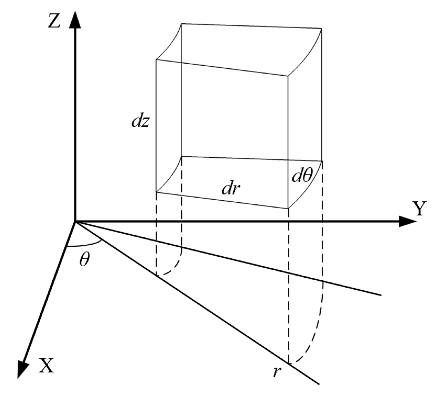
2.4. Boundary Condition Analysis

Assuming that the depths of the various geological stratifications within the Earth are the same, the geometry of the Earth’s interior, the constraints, and the loads acting on it are all symmetrical on a fixed axis pointing towards the center of the Earth from the overshooting source. Axisymmetric cylindrical coordinates $(r,\theta ,z)$ are typically employed in this context, as illustrated in Figure 3. With the axis of symmetry designated as the $z$-axis, all stresses, strains, and displacements are independent of the $\theta$-direction and are solely a function of $r$ and $z$. The displacement at any given point can be expressed as a sum of two directional components: a radial displacement along the $r$-direction and an axial displacement along the $z$-direction.

If the positive stress on the inner cylindrical face of a hexahedron is ${\sigma }_r$, the positive stress on the outer cylindrical face is ${\sigma }_r+(\partial {\sigma }_r/\partial r)dr$. Given the axisymmetry, it can be demonstrated that ${\sigma }_{\theta }$ has no increment in the annular direction. If the positive stress below the hexahedron is designated as ${\sigma }_z$, then the positive stress above should be expressed as ${\sigma }_z+(\partial {\sigma }_z/\partial \mathrm{z})dz$. Similarly, the shear stresses on the inner and outer faces of the hexahedron are ${\tau }_{zr}$ and ${\tau }_{zr}+(\partial {\tau }_{zr}/\partial r)dr$, respectively. The shear stresses on the underside and the top are ${\tau }_{rz}$ and ${\tau }_{rz}+(\partial {\tau }_{rz}/\partial z)dz$, respectively. Furthermore, the radial body force is represented by $F_r$, and the axial body force is represented by $F_z$. If all the forces on the hexahedron are projected onto the radial axis at the center of the hexahedron and are taken to be s $\mathrm{s}\mathrm{i}\mathrm{n}(d\theta /2)\approx d\theta /2$ and cos $\mathrm{c}os(d\theta /2)\approx 1$. The equilibrium equation in the $r$ direction can be obtained:

$$\begin{array}{c}\left({\sigma }_r+{\displaystyle \frac{\partial {\sigma }_r}{\partial r}}dr\right)(r+dr)d\theta dz-{\sigma }_{r}rd\theta dz-{\sigma }_{\theta }drdz{\displaystyle \frac{d\theta }{2}}-{\sigma }_{\theta }drdz{\displaystyle \frac{d\theta }{2}}\\ +\left({\tau }_{rz}+{\displaystyle \frac{\partial {\tau }_{rz}}{\partial z}}dz\right)rd\theta dr-{\tau }_{rz}rd\theta dr+F_{r}rd\theta drdz=0\end{array}$$

(13)

Similarly, the equilibrium equation in the $z$-direction is obtained:

$$\begin{array}{c}\left({\tau }_{rz}+{\displaystyle \frac{\partial {\tau }_{rz}}{\partial r}}dr\right)\left(r+dr\right)d\theta dz-{\tau }_{rz}rd\theta dz\\ +\left({\sigma }_z+{\displaystyle \frac{\partial {\sigma }_z}{\partial z}}dz\right)rd\theta dr-{\sigma }_{z}rd\theta dr+F_{z}rd\theta drdz=0\end{array}.$$

(14)

Ignoring the second-order small quantities, the equilibrium differential equation can be expressed as

$$\left\{\begin{array}{c}{\displaystyle \frac{\partial {\sigma }_r}{\partial r}}+{\displaystyle \frac{\partial {\tau }_{zr}}{\partial z}}+{\displaystyle \frac{{\sigma }_r-{\sigma }_{\theta }}{r}}+F_r=0\\ {\displaystyle \frac{\partial {\sigma }_z}{\partial z}}+{\displaystyle \frac{\partial {\tau }_{zr}}{\partial r}}+{\displaystyle \frac{{\tau }_{zr}}{r}}+F_z=0\end{array}\right.$$

(15)

According to Equations (13)–(15), numerical simulations can be calculated using the axisymmetric model.

3. Numerical Simulation

3.1. Numerical Modeling of Deep Earthquake

The LS-DYNA 970 module of ANSYS-19.0 is employed for numerical simulation [47,48]. For computational efficiency, the geological structure is modeled as an axisymmetric spatial representation. Figure 4 provides a detailed illustration of the model structure and parameters. This model spans a horizontal length of 400 km and descends to a depth of 730 km. These dimensions were specifically selected to effectively observe seismic-wave propagation while optimizing computational resources. Vertically, it is segmented into six layers. The crust has two layers: a granite layer (20 km) followed by a basalt layer (16 km). The upper mantle is divided into four layers, from top to bottom: the lithospheric mantle (24 km), the asthenosphere (160 km), the B-layer transition zone (190 km), and the C-layer transition zone (320 km). The epicenter of the earthquake is located in the C-layer transition zone at a depth of 578 km.

The left boundary of the model represents the axis of symmetry. Axisymmetric boundary conditions are defined by Axisymmetric Solid Element Formulation in the *SECTION_SHELL keyword. Free boundary conditions are set on the top edge, while non-reflecting boundary conditions are applied to the right and bottom edges using the *BOUNDARY_NON_REFLECTING keyword. The energy release source in the model corresponds to a TNT explosion characterized by a pressure density of 1.63 g/cm³ and a total mass of 336,000 tons [49]. In the TNT simulations, the Arbitrary Lagrangian–Eulerian (ALE) algorithm elements are employed to accurately simulate the dynamic response of materials [50,51]. The fluid–structure coupling method is utilized to govern interactions within the C-layer transition zone. Except for the TNT region, Lagrangian elements are employed in other areas. The interaction between layers is managed using common nodes, thereby ensuring continuity in metrics of displacement, velocity, and acceleration. It takes about 30 h on a 20-core computer to run the model in this study.

To characterize the seismic wave generated by the detonation of TNT explosives, the high explosive intrinsic model (keyword *MAT_HIGH_EXPLOSIVE_BURN) and the Jones–Wilkins–Lee equation of state (keyword *EOS_JWL) are employed. The pressure can be expressed as

$$P=A_{jwl}\left(1-{\displaystyle \frac{{\omega }_{jwl}}{R_{1jwl}V}}\right)e^{-R_{1jwl}{V}_{jwl}}+B_{jwl}\left(1-{\displaystyle \frac{{\omega }_{jwl}}{R_{2jwl}{V}_{jwl}}}\right)e^{-R_{2jwl}{V}_{jwl}}+{\displaystyle \frac{{\omega }_{jwl}{E}_{jwl}}{E_{jwl}}}$$

(16)

where P is the pressure, $E_{jwl}$ is the initial internal energy, $V_{jwl}$ is the relative volume, and $A_{jwl}$, $B_{jwl}$, $R_{1jwl}$, $R_{2jwl}$, and ${\omega }_{jwl}$ are the material constants. The relevant parameters of the TNT model are shown in

Table 1. Material parameters of TNT [52].

$\mathit{\rho }$ (kg·m−3)	$\mathit{D}$ (m·s−1)	${\mathit{P}}_{\mathit{J}\mathit{C}}$ (GPa)	${\mathit{A}}_{\mathit{j}\mathit{w}\mathit{l}}$ (GPa)	${\mathit{B}}_{\mathit{j}\mathit{w}\mathit{l}}$ (GPa)	${\mathit{R}}_{1\mathit{j}\mathit{w}\mathit{l}}$	${\mathit{R}}_{2\mathit{j}\mathit{w}\mathit{l}}$	${\mathit{\omega }}_{\mathit{j}\mathit{w}\mathit{l}}$	${\mathit{E}}_0$ (J·m−3)
1630	6930	27	371	0.743	4.15	0.95	0.3	$1\times {10}^9$

[52].

The velocities $V_p$ and $V_s$ are determined using Equation (17),

$$\begin{array}{c}{V}_p=\sqrt{{\displaystyle \frac{K}{\rho }}}\\ V_s=\sqrt{{\displaystyle \frac{G}{\rho }}}\end{array},$$

(17)

where $V_p$ is the longitudinal wave velocity; $V_s$ is the shear wave velocity; $K$ is the elastic modulus; G is the shear modulus; and $\rho$ is the density [53].

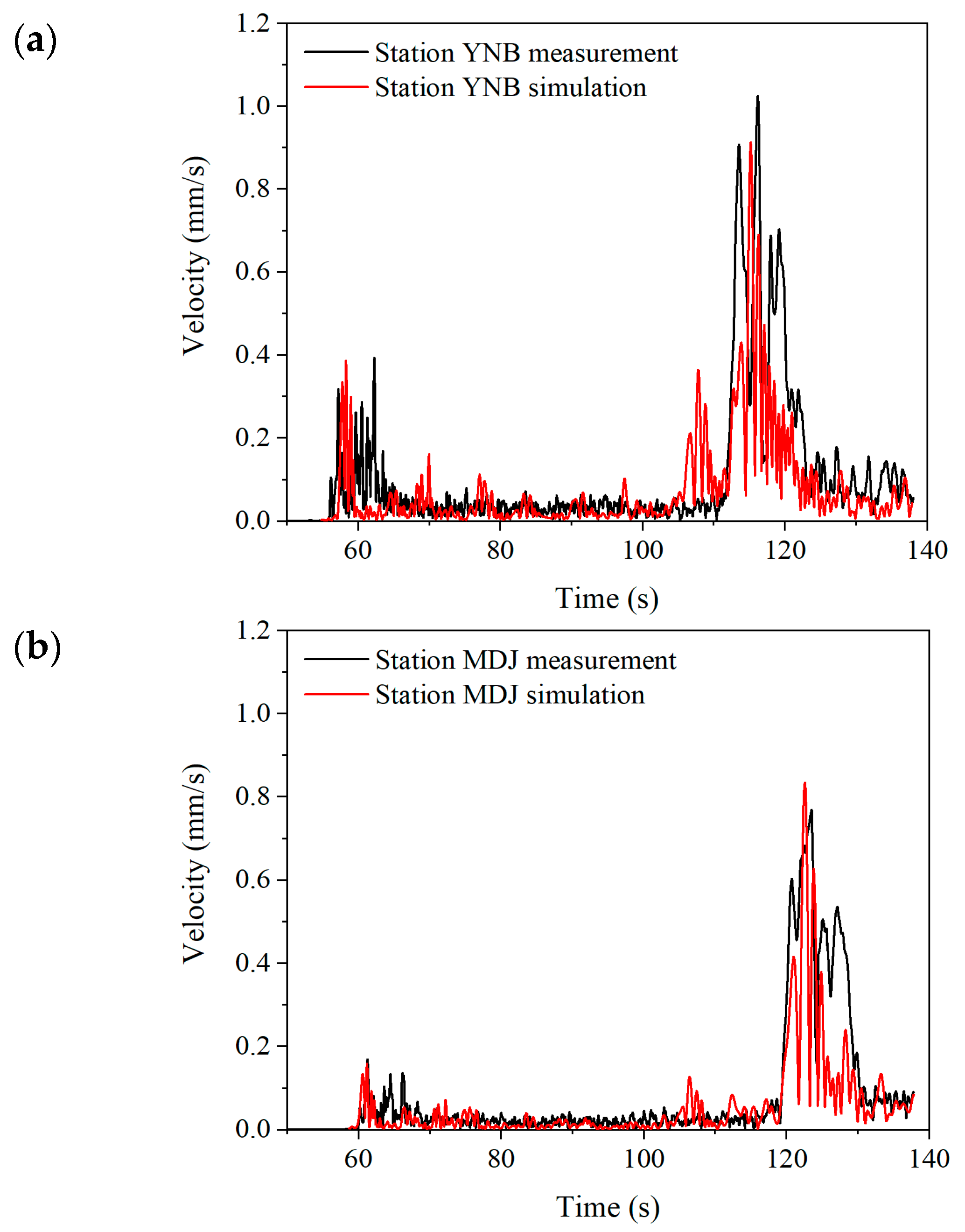
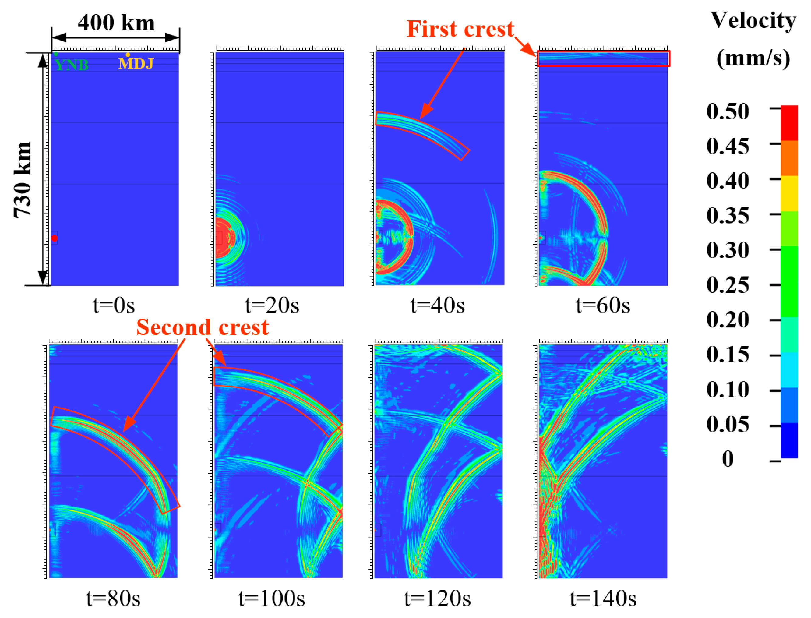
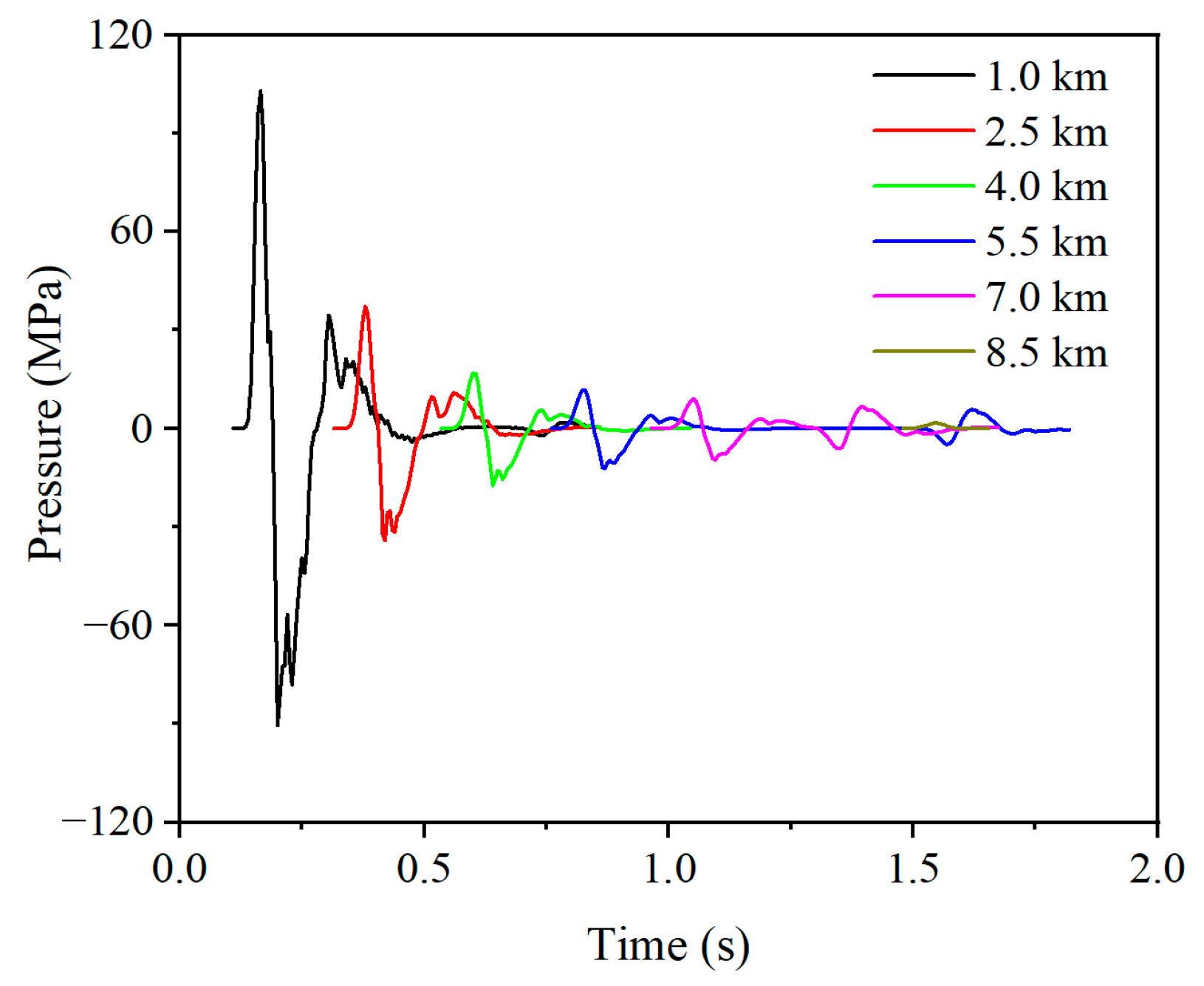
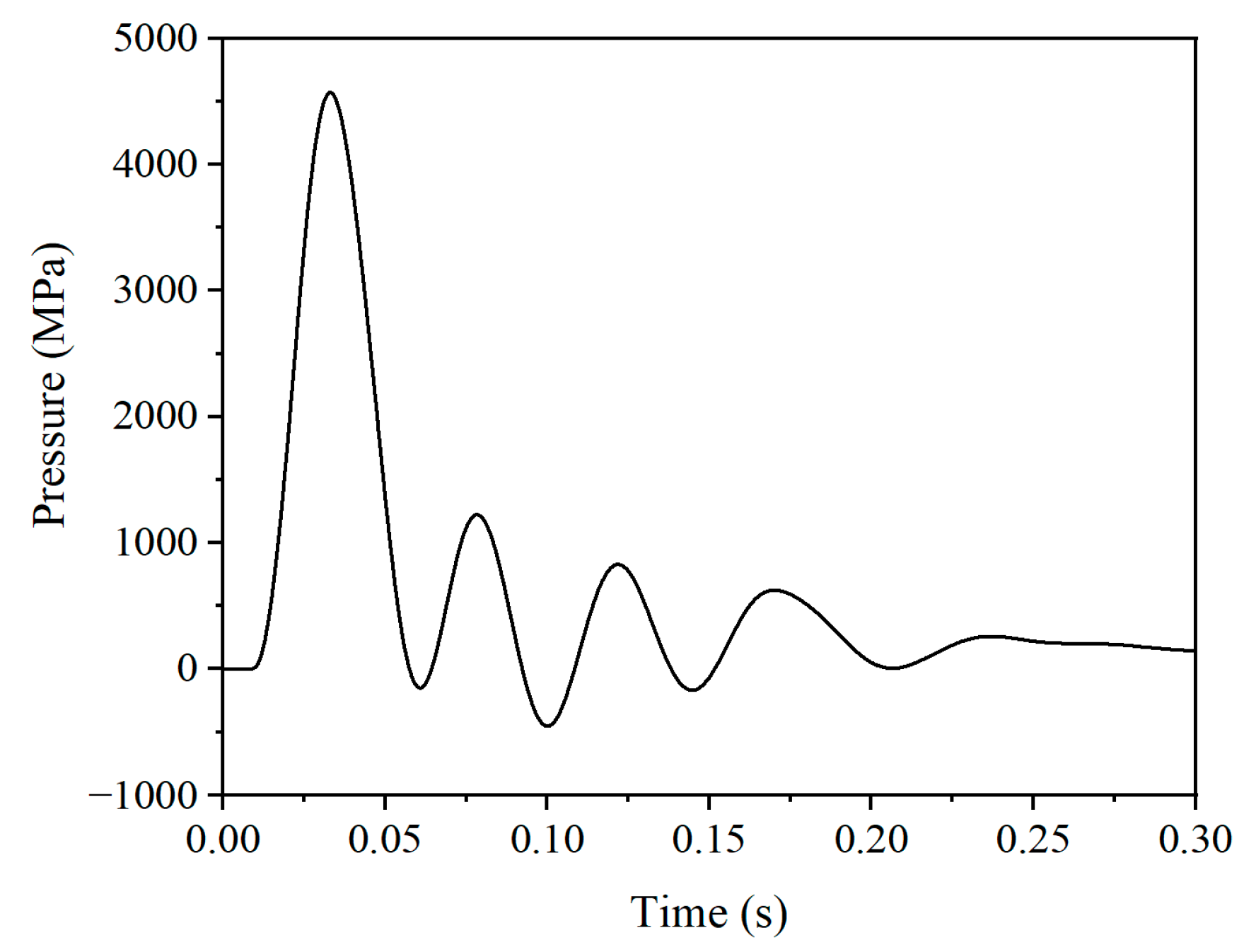
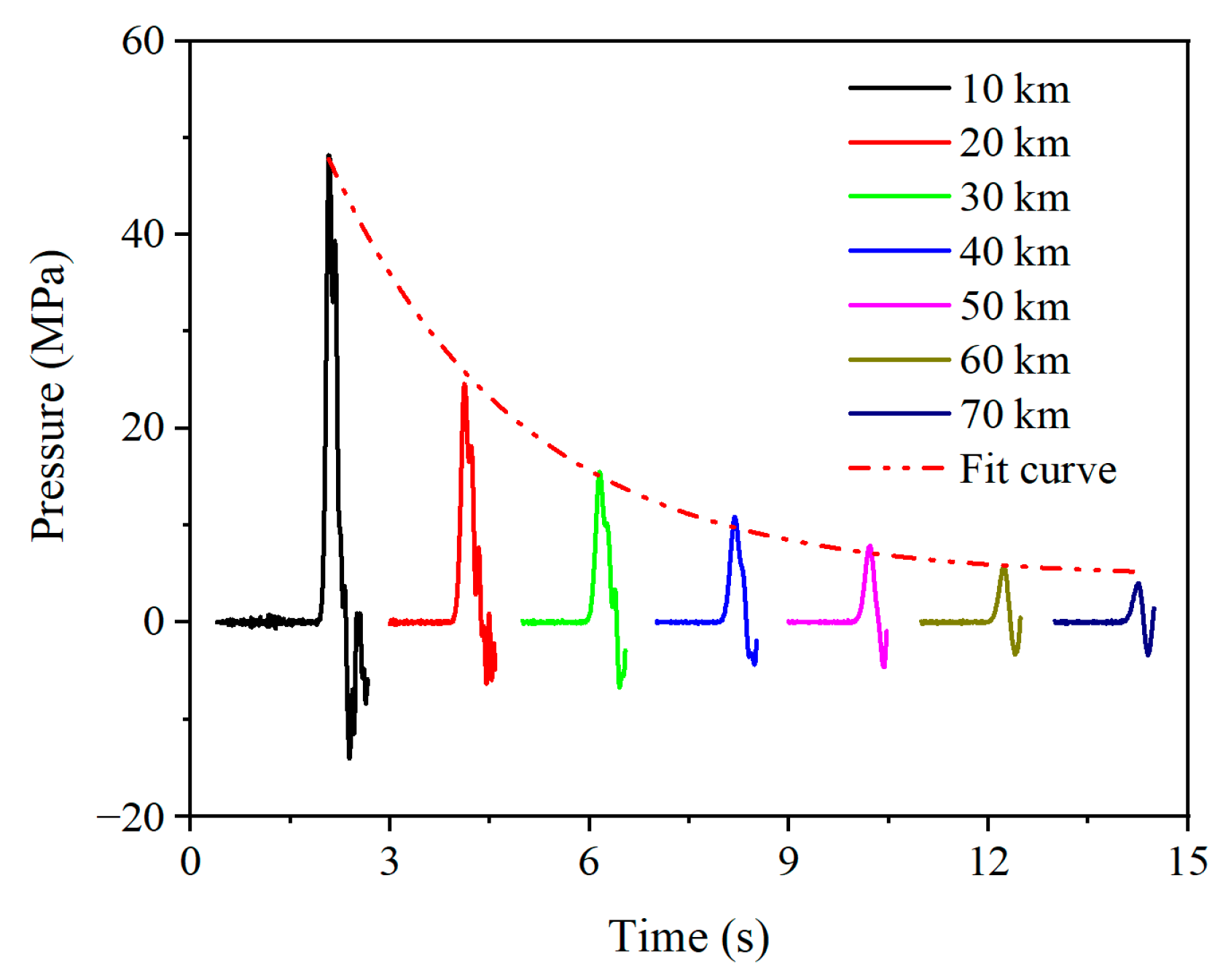
3.2. Numerical Results

The results from the numerical simulation are contrasted against velocities recorded by the YNB and MDJ seismic stations. Figure 5 presents this comparison, and the velocity evolution based on the numerical simulation is portrayed in Figure 6.

As illustrated in Figure 5, the results demonstrate a high degree of alignment between the simulated and observed data, both in terms of wave arrival times and amplitude in velocities. For instance, the discrepancy between the observed and simulated peak amplitude in velocities at the YNB and MDJ seismic stations within specific timeframes remains below 9%. The results indicate that, for the specific earthquake source and area under consideration, a TNT explosion can effectively simulate seismic energy propagation. However, it is important to confirm this applicability whenever the source characteristics or site conditions vary, as both source parameters, such as fracture dynamics, and site characteristics significantly influence peak ground velocity.

Figure 7 showcases the stress distribution at distances extending 45° horizontally from the epicenter, positioned 578 km below the surface. The relationship between distance and stress, derived from numerical simulation results, is shown in Equation (18), highlighting an exponential power decrease in stress amplitude with increasing distance:

$$\mathsf{\sigma }=60.1\times d^{-1.32},$$

(18)

where $\mathsf{\sigma }$ is the effective stress and $d$ is the distance from the hypocenter.

4. Methodological Extension

4.1. Explosion Response of Water and Layered Geological Structures Models

4.1.1. Numerical Modeling of Layered Geological Structures

Figure 8 presents various numerical explosion models developed for certain geologies: water and layered geological structures. These models facilitate a comprehensive understanding of stress-wave propagation and attenuation patterns, as well as stress-state features, as these can be influenced by the specific geological medium. Four equivalent simulated explosions are considered, reflecting earthquake surface-wave magnitudes of 7.5. Based on Equation (1), these magnitudes correspond to the energy release equivalent to the detonation of 2,212,100 tons of TNT [29].

Specifically, the numerical models for the various geologies are as follows:

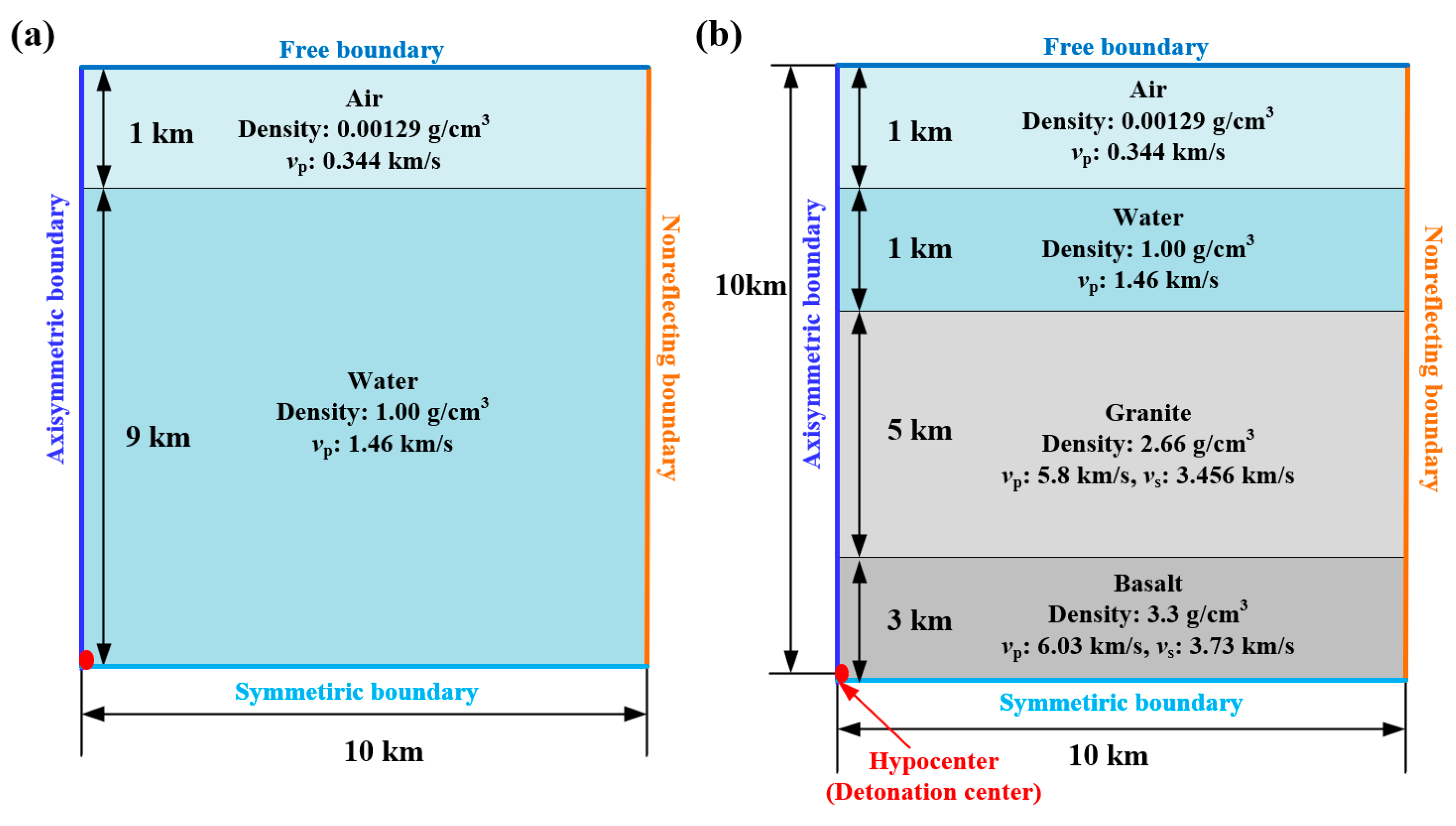
• Water Model (Figure 8a): This spatially axisymmetric model simulates the seismic-wave attenuation behavior of water at a 9 km depth across the given magnitudes. The model incorporates an air layer 1 km high, effectively representing a water body of 9 km depth and a 10 km radius.
• Three-Layered Medium (Figure 8b): This model explores responses in a tri-layered structure: an upper water layer 1 km deep, a middle granite layer 5 km deep, and a lower basalt layer 3 km deep. An air layer of 1 km is added above this structure.

Specifically, the mechanical parameters for the various media are as follows:

• Air: Density of 1.29 kg/m³ and $V_p$ of 0.344 km/s [54].
• Water: Density of 1000 kg/m³ and $V_p$ of 1.46 km/s [54].
• Granite: Density of 2660 kg/m³, $V_p$ of 5.8 km/s, and $V_s$ of 3.456 km/s [35,36].
• Basalt: Density of 3300 kg/m³, $V_p$ of 6.03 km/s, and $V_s$ of 3.73 km/s [35,36].

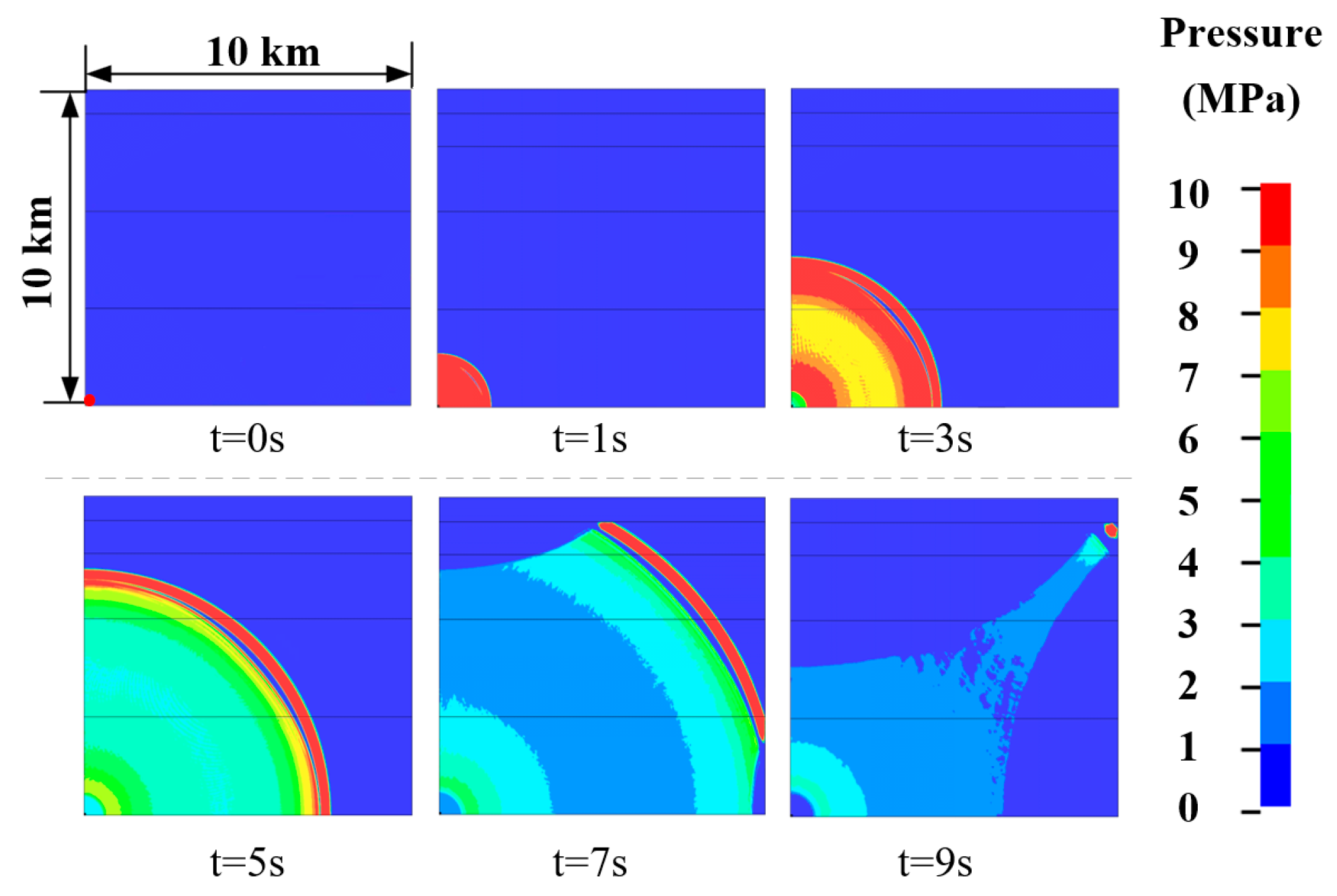
4.1.2. Numerical Results for Water

Figure 9 visualizes the pressure distributions resulting from underwater explosions, showcasing how stress propagates in water. A review of the distributions reveals that, except for compressive stress, all other forms of stress are insignificant during the propagation of the stress wave. This is a characteristic behavior of water, an inviscid fluid, which can only bear compressive stress and is incapable of withstanding tensile or shear stress.

Figure 10a illustrates the temporal stress variations at varying distances from the source in water. The peak compressive stress values recorded at distances of 1, 2.5, 4.0, 5.5, 7.0, and 8.5 km are 68.7, 22.0, 12.2, 8.2, 5.95, and 4.65 MPa, respectively. The corresponding arrival times for these stress values are 0.64 s, 1.68 s, 2.71 s, 3.75 s, 4.76 s, and 5.81 s. Notably, at a distance of 9 km (which represents the upper water surface), stress unloading occurs. This effectively means a zero-stress zone is present due to the free surface conditions. Figure 10b presents a fitted exploration into the attenuation properties of seismic waves across water, based on data points extracted from numerical simulations. As illustrated in Figure 10b, the attenuation pattern of stress waves in water exhibits exponential decay. This also demonstrates that the model is capable of responding to the laws of seismic-wave propagation within geological structures, thereby validating the numerical simulation model.

4.1.3. Numerical Results of Layered Geological Structures Models

Figure 11 provides insights into the stress propagation within the underwater granite and basalt geology. One crucial observation is the impact of the interface between granite and basalt. When the stress wave encounters this boundary, a portion of it reflects, while the rest transmits into the granite medium. The magnitude of reflection here is lesser compared to that at the fluid-solid interface. This can be attributed to the relatively minimal wave impedance difference between granite and basalt. Consequently, the energy of the stress wave transitions more smoothly between these two solid mediums. As the stress wave encounters the boundary between the water and granite, it splits: a portion transmits into the adjacent medium, while the remainder reflects into the original one. Given the juxtaposition of solid basalt and fluidic water, only compressive stress moves into the water as the wave progresses from granite. A significant reflection can be observed at the interface, primarily because of the stark contrast between the wave impedance of water and that of granite.

Figure 12 depicts the interaction between stress and time at varying distances from the epicenter. An intriguing pattern emerges at the 1 km distance, where a minor stress-wave fluctuation is evident around 0.75 s. This phenomenon can be attributed to the reflective action occurring at the granite–basalt interface. However, due to the minimal impedance gap between the two solid media, the reflection remains relatively subdued. It is important to note that the difference in wave impedance between granite and basalt affects the behavior of reflected and refracted energy.

At a greater depth of 7 km, the waveform undergoes a distinct evolution. The initial stress wave peaks at approximately 1.05 s, with a peak value of 8.93 MPa. Subsequently, a reflected wave is observed at 1.35 s, reaching a peak value of 6.19 MPa. This pronounced reflection is a direct consequence of the considerable wave impedance disparity between granite and water, resulting in the majority of the stress wave rebounding at the interface.

4.2. Numerical Analysis of the Equivalent Explosion Response

Earthquake depth and magnitude play critical roles when assessing seismic sources. A significant majority, in fact over 90%, of global seismic activities are categorized as shallow earthquakes, characterized by a focal depth less than 70 km [55,56].

To delve into the nuances of seismic-wave propagation within a gradient geological structure, a two-dimensional planar model is introduced, as seen in Figure 13. With its hypocenter hosting a load equivalent to a predetermined pressure load, the model spreads 80 km horizontally and dives 6 km in depth. This vertical geology is segmented into a single layer. Pressure is then applied at the designated loading point, facilitating an exploration into seismic-wave propagation patterns across various media.

Using granite as a representative medium, its attributes include a density of 2.66 g/cm³, a $V_{\mathrm{p}}$ of 5.8 km/s, and a $V_{\mathrm{s}}$ of 3.456 km/s. Figure 14 portrays the pressure–time curve applied at the load point. This curve’s characteristics are evocative of the pressure generated by ambient material during a TNT detonation [57]. The curve’s inaugural cycle loading boasts a width of 0.05 s, with a zenith of 4560 MPa at the 0.033 s mark. Ensuing wave crests undergo exponential decline, with peaks recorded at 1220 MPa, 830 MPa, and 620 MPa, with their timestamps being 0.079 s, 0.122 s, and 0.170 s, respectively. After this, the pressure gradually stabilizes and starts a slow decline.

Figure 15 presents the pressure states and their respective fitting curves at various distances from the load point. These distances encompass points 10, 20, 30, 40, 50, 60, and 70 km to the right in the horizontal trajectory. Meanwhile, Figure 16 shows the pressure variances across the seismic-wave propagation process. For these distances, pressure values at 48.21, 24.58, 15.49, 10.80, 7.88, 5.73, and 4.02 MPa, in sequence. The coinciding arrival times span 2.08, 4.12, 6.15, 8.19, 10.22, 12.24, and 14.26 s, with pulse widths distributed across 0.44, 0.41, 0.42, 0.40, 0.37, 0.33, and 0.27 s. Notably, with an increment in distance, stress amplitude displays a brisk decay between 10 to 40 km, but this rate of decay tapers off within the 40 to 70 km range.

5. Conclusions

This research introduces a new numerical simulation method for simulating the seismic-wave propagation in geological structures during earthquakes by using the TNT energy release process. This new approach allows for the modeling of energy discharge in seismic sources in a manner analogous to TNT explosions, providing new insights into the dynamics of seismic waves in geological settings. The feasibility and accuracy of this model have been demonstrated by comparing simulated results with actual seismic data from the 2012 Northeast China earthquake.

The capability of the simulation to reproduce the seismic-wave propagation process within varied geological structures, including water and layered geological configurations, has been validated. This facilitates a deeper comprehension of wave propagation and attenuation laws in these settings. The results presented in Section 3.2 substantiate the suitability of the geological parameters employed and their efficacy in accurately simulating seismic-wave propagation.

Furthermore, an equivalent blast load model was established through numerical simulations, thereby facilitating an exhaustive examination of seismic-wave propagation in singular media within shallow geologies. Uncovering the propagation characteristics and attenuation laws of these seismic waves has strengthened the foundation for future exploration of seismic-wave propagation in shallow, complex geological structures.

However, it should be noted that the simulation model in this study is based on the assumption that the geological structure of the medium is homogeneous, which is limited to simulating the wave propagation within a homogeneous geological structure or obtaining the approximate results for the complex geological structure. To face more complex geological conditions, many influencing factors, such as the inhomogeneity of the geological structure and complex boundary conditions, need to be considered in the simulation model in future work.

References

1. Karato, S.-I.; Jung, H.; Katayama, I.; Skemer, P. Geodynamic significance of seismic anisotropy of the upper mantle: New insights from laboratory studies. Annu. Rev. Earth Planet. Sci. 2008, 36, 59–95. [Google Scholar] [CrossRef]
2. Russo, R.M.; Silver, P.G. Trench-parallel flow beneath the nazca plate from seismic anisotropy. Science 1994, 263, 1105–1111. [Google Scholar] [CrossRef] [PubMed]
3. Virieux, J.; Operto, S. An overview of full-waveform inversion in exploration geophysics. Geophysics 2009, 74, WCC1–WCC26. [Google Scholar] [CrossRef]
4. Zhu, H.; Stern, R.J.; Yang, J. Seismic evidence for subduction-induced mantle flows underneath Middle America. Nat. Commun. 2020, 11, 2075. [Google Scholar] [CrossRef]
5. Brossier, R.; Operto, S.; Virieux, J. Seismic imaging of complex onshore structures by 2D elastic frequency-domain full-waveform inversion. Geophysics 2009, 74, WCC105–WCC118. [Google Scholar] [CrossRef]
6. Tromp, J. Seismic wavefield imaging of Earth’s interior across scales. Nat. Rev. Earth Environ. 2020, 1, 40–53. [Google Scholar] [CrossRef]
7. Harris, C.W.; Miller, M.S.; Porritt, R.W. Tomographic Imaging of Slab Segmentation and Deformation in the Greater Antilles. Geochem. Geophys. Geosyst. 2018, 19, 2292–2307. [Google Scholar] [CrossRef]
8. Pageot, D.; Operto, S.; Vallée, M.; Brossier, R.; Virieux, J. A parametric analysis of two-dimensional elastic full waveform inversion of teleseismic data for lithospheric imaging. Geophys. J. Int. 2013, 193, 1479–1505. [Google Scholar] [CrossRef]
9. Gélis, C.; Virieux, J.; Grandjean, G. Two-dimensional elastic full waveform inversion using Born and Rytov formulations in the frequency domain. Geophys. J. Int. 2007, 168, 605–633. [Google Scholar] [CrossRef]
10. Chi, B.; Dong, L.; Liu, Y. Full waveform inversion method using envelope objective function without low frequency data. J. Appl. Geophys. 2014, 109, 36–46. [Google Scholar] [CrossRef]
11. Zhu, H.; Yang, J.; Li, X. Azimuthal Anisotropy of the North American Upper Mantle Based on Full Waveform Inversion. J. Geophys. Res. Solid Earth 2020, 125, 18432. [Google Scholar] [CrossRef]
12. Zhang, J.; Toksöz, M.N. Nonlinear refraction traveltime tomography. Geophysics 1998, 63, 1726–1737. [Google Scholar] [CrossRef]
13. Taillandier, C.; Noble, M.; Chauris, H.; Calandra, H. First-arrival traveltime tomography based on the adjoint-state method. Geophysics 2009, 74, WCB1–WCB10. [Google Scholar] [CrossRef]
14. Almuhaidib, A.M.; Toksoez, M.N. Finite difference elastic wave modeling with an irregular free surface using ADER scheme. J. Geophys. Eng. 2015, 12, 435–447. [Google Scholar] [CrossRef]
15. Kristeková, M.; Kristek, J.; Moczo, P. Time-frequency misfit and goodness-of-fit criteria for quantitative comparison of time signals. Geophys. J. Int. 2009, 178, 813–825. [Google Scholar] [CrossRef]
16. Shragge, J.; Konuk, T. Tensorial elastodynamics for isotropic media. Geophysics 2020, 85, T359–T373. [Google Scholar] [CrossRef]
17. Wang, Y.; Zhang, J. Joint refraction traveltime tomography and migration for multilayer near-surface imaging. Geophysics 2019, 84, U31–U43. [Google Scholar] [CrossRef]
18. Manakou, M.; Raptakis, D.; Chávez-García, F.; Apostolidis, P.; Pitilakis, K. 3D soil structure of the Mygdonian basin for site response analysis. Soil Dyn. Earthq. Eng. 2010, 30, 1198–1211. [Google Scholar] [CrossRef]
19. Huang, H.; Zhang, Z.; Chen, X. Investigation of topographical effects on rupture dynamics and resultant ground motions. Geophys. J. Int. 2018, 212, 311–323. [Google Scholar] [CrossRef]
20. Zang, N.; Zhang, W.; Chen, X. An overset-grid finite-difference algorithm for simulating elastic wave propagation in media with complex free-surface topography. Geophysics 2021, 86, T277–T292. [Google Scholar] [CrossRef]
21. Komatitsch, D.; Tromp, J. Introduction to the spectral element method for three-dimensional seismic wave propagation. Geophys. J. Int. 1999, 139, 806–822. [Google Scholar] [CrossRef]
22. Etienne, V.; Chaljub, E.; Virieux, J.; Glinsky, N. An hp-adaptive discontinuous Galerkin finite-element method for 3-D elastic wave modelling. Geophys. J. Int. 2010, 183, 941–962. [Google Scholar] [CrossRef]
23. Wang, D.; Qin, X.; Chen, W.; Wang, S. Simulation of the Deformation and Failure Characteristics of a Cylinder Shell under Internal Explosion. Appl. Sci. 2022, 12, 1217. [Google Scholar] [CrossRef]
24. Kim, S.; Jang, T.; Oli, T.; Park, C. Behavior of Barrier Wall under Hydrogen Storage Tank Explosion with Simulation and TNT Equivalent Weight Method. Appl. Sci. 2023, 13, 3744. [Google Scholar] [CrossRef]
25. Hung, C.-W.; Lai, H.-H.; Shen, B.-C.; Wu, P.-W.; Chen, T.-A. Development and Validation of Overpressure Response Model in Steel Tunnels Subjected to External Explosion. Appl. Sci. 2020, 10, 6166. [Google Scholar] [CrossRef]
26. Gong, C.; Qiu, Y.-Y.; Long, Z.-L.; Liu, L.; Xu, G.-G.; Yang, L.-M. Study on the Earth-Covered Magazine Models under the Internal Explosion. Shock. Vib. 2024, 2024, 1–20. [Google Scholar] [CrossRef]
27. Zhang, H.; Jia, Z.; Ye, Q.; Cheng, Y.; Li, S. Numerical simulation on influence of initial pressures on gas explosion propagation characteristics in roadway. Front. Energy Res. 2022, 10, 913045. [Google Scholar] [CrossRef]
28. Hu, Y.; Lu, W.; Wu, X.; Liu, M.; Li, P. Numerical and experimental investigation of blasting damage control of a high rock slope in a deep valley. Eng. Geol. 2018, 237, 12–20. [Google Scholar] [CrossRef]
29. Choy, G.L.; Boatwright, J.L. Global patterns of radiated seismic energy and apparent stress. J. Geophys. Res.-Solid Earth 1995, 100, 18205–18228. [Google Scholar] [CrossRef]
30. Chen, J.; Jiang, L.; Li, J.; Shi, X. Numerical simulation of shaking table test on utility tunnel under non-uniform earthquake excitation. Tunn. Undergr. Space Technol. 2012, 30, 205–216. [Google Scholar] [CrossRef]
31. Wolfe, C.J.; Silver, P.G. Seismic anisotropy of oceanic upper mantle: Shear wave splitting methodologies and observations. J. Geophys. Res.-Solid Earth 1998, 103, 749–771. [Google Scholar] [CrossRef]
32. Salah, M.K.; Alqudah, M.; El-Aal, A.K.A.; Barnes, C. Effects of porosity and composition on seismic wave velocities and elastic moduli of lower cretaceous rocks, central Lebanon. Acta Geophys. 2018, 66, 867–894. [Google Scholar] [CrossRef]
33. Olson, P.; Reynolds, E.; Hinnov, L.; Goswami, A. Variation of ocean sediment thickness with crustal age. Geochem. Geophys. Geosystems 2016, 17, 1349–1369. [Google Scholar] [CrossRef]
34. Li, F.; Sun, Z.; Zhang, J. Influence of mid-crustal rheology on the deformation behavior of continental crust in the continental subduction zone. J. Geodyn. 2018, 117, 88–99. [Google Scholar] [CrossRef]
35. Liu, M.; Cui, X.J.; Liu, F.T. Cenozoic rifting and volcanism in eastern China: A mantle dynamic link to the Indo-Asian collision? Tectonophysics 2004, 393, 29–42. [Google Scholar] [CrossRef]
36. Song, B.; Nutman, A.P.; Liu, D.; Wu, J. 3800 to 2500 Ma crustal evolution in the Anshan area of Liaoning Province, northeastern China. Precambrian Res. 1996, 78, 79–94. [Google Scholar] [CrossRef]
37. Chen, Y.-W.; Colli, L.; Bird, D.E.; Wu, J.; Zhu, H. Caribbean plate tilted and actively dragged eastwards by low-viscosity asthenospheric flow. Nat. Commun. 2021, 12, 1603. [Google Scholar] [CrossRef]
38. Wolf, J.; Long, M.D.; Leng, K.; Nissen-Meyer, T. Constraining deep mantle anisotropy with shear wave splitting measurements: Challenges and new measurement strategies. Geophys. J. Int. 2022, 230, 507–527. [Google Scholar] [CrossRef]
39. Levin, V.; Elkington, S.; Bourke, J.; Arroyo, I.; Linkimer, L. Seismic anisotropy in southern Costa Rica confirms upper mantle flow from the Pacific to the Caribbean. Geology 2021, 49, 8–12. [Google Scholar] [CrossRef]
40. Schellart, W.P. Kinematics of subduction and subduction-induced flow in the upper mantle. J. Geophys. Res.-Solid Earth 2004, 109, B07401. [Google Scholar] [CrossRef]
41. Feng, Z.-Q.; Jia, C.-Z.; Xie, X.-N.; Zhang, S.; Feng, Z.-H.; Cross, T.A. Tectonostratigraphic units and stratigraphic sequences of the nonmarine Songliao basin, northeast China. Basin Res. 2010, 22, 79–95. [Google Scholar]
42. Feng, M.; An, M.; Hou, H.; Fan, T.; Zang, H. Channelised magma ascent and lithospheric zonation beneath the Songliao Basin, Northeast China, based on surface-wave tomography. Tectonophysics 2023, 862, 229969. [Google Scholar] [CrossRef]
43. Lu, Q.; Wang, Z.-J. Studies of the propagation of viscoelastic spherical divergent stress waves based on the generalized Maxwell model. J. Sound Vib. 2016, 371, 183–195. [Google Scholar] [CrossRef]
44. Towfighi, S.; Kundu, T. Elastic wave propagation in anisotropic spherical curved plates. Int. J. Solids Struct. 2003, 40, 5495–5510. [Google Scholar] [CrossRef]
45. Sun, C.; Li, C.; Wei, X. Research on Seismic Wave Quality Factor of Marble Jointed Rock Mass under SHPB Impact. Appl. Sci. 2022, 12, 10875. [Google Scholar] [CrossRef]
46. Gu, Z.; Wei, C.; Wu, X.; Huang, C. Laser-induced shock response of shear thickening fluid. Acta Mech. Sin. 2023, 39, 123118. [Google Scholar]
47. Gu, Z.; Wu, X.; Li, Q.; Yin, Q.; Huang, C. Dynamic compressive behaviour of sandwich panels with lattice truss core filled by shear thickening fluid. Int. J. Impact Eng. 2020, 143, 103616. [Google Scholar] [CrossRef]
48. Gu, Z.; Cheng, Y.; Xiao, K.; Li, K.; Wu, X.; Li, Q.; Huang, C. Geometrical scaling law for laser-induced micro-projectile impact testing. Int. J. Mech. Sci. 2022, 223, 107289. [Google Scholar] [CrossRef]
49. Goswami, A.; Ganesh, T.; Adhikary, S.D. RC structures subjected to combined blast and fragment impact loading: A state-of-the-art review on the present and the future outlook. Int. J. Impact Eng. 2022, 170, 104355. [Google Scholar] [CrossRef]
50. Barlow, A.J.; Maire, P.-H.; Rider, W.J.; Rieben, R.N.; Shashkov, M.J. Arbitrary Lagrangian-Eulerian methods for modeling high-speed compressible multimaterial flows. J. Comput. Phys. 2016, 322, 603–665. [Google Scholar] [CrossRef]
51. Richter, T.; Wick, T. Finite elements for fluid-structure interaction in ALE and fully Eulerian coordinates. Comput. Methods Appl. Mech. Eng. 2010, 199, 2633–2642. [Google Scholar] [CrossRef]
52. Liu, D.; Dai, C.; Yu, C.; Ma, Y. Numerical Simulation and Experimental Study on Single Point Blasting of Ice Jam of Heilongjiang River Based on ANSYS/LSDYNA. Water 2022, 14, 2808. [Google Scholar] [CrossRef]
53. Phani, K.K. Estimation of elastic properties of porous ceramic using ultrasonic longitudinal wave velocity only. J. Am. Ceram. Soc. 2007, 90, 2165–2171. [Google Scholar] [CrossRef]
54. Wang, Z.-L.; Li, Y.-C.; Shen, R. Numerical simulation of tensile damage and blast crater in brittle rock due to underground explosion. Int. J. Rock Mech. Min. Sci. 2007, 44, 730–738. [Google Scholar] [CrossRef]
55. Ma, Y.; Hale, D. Wave-equation reflection traveltime inversion with dynamic warping and full-waveform inversion. Geophysics 2013, 78, R223–R233. [Google Scholar] [CrossRef]
56. Scholz, C.H. Earthquakes and friction laws. Nature 1998, 391, 37–42. [Google Scholar] [CrossRef]
57. Wang, C.-H.; Wang, S.-S.; Zhang, J.-X. Pressure Load Characteristics of Nonideal Explosives in a Simulation Cabin. Shock. Vib. 2019, 2019, 6862134. [Google Scholar] [CrossRef]
Figure 1. Geographic positions of the hypocenter (130.703° E, 42.587° N) and the nearby YNB and MDJ seismic stations for the 18 February 2012, seismic event.
Applsci 14 08278 g001
Figure 2. The seismic-wave amplitude in velocities (combined velocities of seismic waves traveling in three directions). Time = 0 s corresponds to the onset of the seismic event.
Applsci 14 08278 g002
Figure 3. Analyzing microelements for spatial axisymmetric problems.
Applsci 14 08278 g003
Figure 4. Schematic diagram of the numerical model.
Applsci 14 08278 g004
Figure 5. Comparison of measured and simulated amplitude in velocities at (a) YNB and (b) MDJ seismic stations.
Applsci 14 08278 g005
Figure 6. Seismic-wave amplitudes in the velocity distribution from the numerical simulation.
Applsci 14 08278 g006
Figure 7. Stress distribution at various distances extending 45° horizontally from the epicenter located 578 km below the surface.
Applsci 14 08278 g007
Figure 8. Schematic representations of numerical explosion models for (a) water and (b) combined underwater granite and basalt.
Applsci 14 08278 g008
Figure 9. Pressure distributions in water from underwater explosions.
Applsci 14 08278 g009
Figure 10. (a) Pressure-time relationship in water at various distances. (b) Variation of peak pressure at different distances from the hypocenter in the water.
Applsci 14 08278 g010
Figure 11. Pressure distributions in underwater granite and basalt.
Applsci 14 08278 g011
Figure 12. Pressure–time relationship of the 7.5 earthquake in underwater basalt at different distances.
Applsci 14 08278 g012
Figure 13. Schematic diagram of the two-dimensional plane model.
Applsci 14 08278 g013
Figure 14. Loading pressure–time relationship.
Applsci 14 08278 g014
Figure 15. Pressure variation at different distances from the loading pressure.
Applsci 14 08278 g015
Figure 16. Pressure distributions of granite at different times.
Applsci 14 08278 g016