Article

Coordinated Planning of Soft Open Points and Energy Storage Systems to Enhance Flexibility of Distribution Networks

1
School of Electric Power, Inner Mongolia University of Technology, Hohhot 010080, China
2
Inner Mongolia Power (Group) Co., Ltd., Inner Mongolia Power Research Institute Branch, Hohhot 010080, China
3
School of Electrical Engineering, Shanghai University of Electric Power, Shanghai 200090, China
*
Authors to whom correspondence should be addressed.
Appl. Sci. 2024, 14(18), 8309; https://doi.org/10.3390/app14188309
Submission received: 8 August 2024 / Revised: 11 September 2024 / Accepted: 12 September 2024 / Published: 14 September 2024
(This article belongs to the Special Issue New Insights into Power Systems)

Abstract

:
With the large-scale penetration of distributed generation (DG), the volatility problems of active distribution networks (ADNs) have become more prominent, which can no longer be met by traditional regulation means and need to be regulated by introducing flexible resources. Soft open points (SOP) and energy storage systems (ESS) can regulate the tidal currents on spatial and temporal scales, respectively, to improve the flexibility of ADN. To this end, in-depth consideration of DG admission is given to establish flexibility assessment indicators from the power side of ADN. The conditional deep convolution generative adversarial network (C-DCGAN) is used to generate the output scenario of DG. On this basis, the SOP and ESS two-layer planning models, which take account of the potential for improvement in the flexibility of ADN, are constructed. Among them, the upper layer is the site selection and volume determination layer, which considers the economy of the system with the optimization objective of minimizing the annual integrated cost; the lower layer is the operation optimization layer, which considers the flexibility of the system and takes the highest average daily flexibility level as the optimization objective. The planning model is solved using genetic algorithm-particle swarm optimization (GA-PSO) and second-order cone programming (SOCP). The case analysis verifies the rationality and effectiveness of the planning model.

1. Introduction

According to the International Energy Agency (IEA), global grid-connected distributed PV capacity will reach 420 GW by the end of 2023, of which China’s grid-connected capacity will reach 254 GW, the European Union 53 GW, and the United States 32 GW. In Denmark, Germany, and other European countries that focus on distributed wind power development, access to the distribution grid of wind power installed capacity accounted for approximately 86.7% of the country’s total installed wind power; in China, the United States, and other countries that focus on centralized wind power development, the cumulative installed capacity of distributed wind power has reached 15.7 GW and 1.1 GW, respectively, and is increasing year by year. With the increasing penetration of DG, their inherent uncertainties and fluctuations will lead to issues such as excessive node voltage, increased network losses, and flexibility constraints on ADN, which cannot be effectively addressed by traditional network regulation methods [1]. SOP [2] and ESS [3] are effective solutions to mitigate these challenges. SOP can provide spatially flexible flow control, while ESS can address the temporal flexibility challenges associated with high penetration of DG [4]. Therefore, the key to resolving these issues lies in how to integrate SOP with ESS, design and coordinate planning strategies effectively, and achieve mutual supplementation of flexible resources, all while balancing the flexibility and economy of ADN.
In recent years, because the large-scale grid integration of DG with uncertainty affects the stable operation of power systems, scholars have conducted research on ADN flexibility. Reference [5] clarifies the definition of operational flexibility and provides a detailed explanation of flexibility supply and flexibility enhancement. Reference [6] analyzes the flexibility resources and introduces the principle of flexibility in supply-demand balance. Reference [7] constructs a flexibility indicator system with flexible resource analysis theory. Reference [8] meets the flexibility demand of the system to cope with uncertainty perturbation by reasonably scheduling flexibility of resource output and eliminates the security risks caused by insufficient flexibility. By reasonably scheduling the flexibility resources, it meets the flexibility demand of the system under the uncertainty disturbance and eliminating the safety hidden danger caused by the lack of flexibility. However, all of the above references are conducted from the perspective of flexibility resource operation optimization under the premise of flexibility resource allocation, without considering the rational planning of flexibility resources. Therefore, with the rapid development of distributed smart grids, it is necessary to study the reasonable and optimal allocation of flexible resources.
SOP, as a network-based flexibility resource, can replace the traditional contact switch to achieve dynamic trend optimization and real-time power regulation in ADN. Reference [9] considered the application of network-type flexibility resource SOP at ADN level and constructed an optimal dispatch model with economy and flexibility as objectives. Reference [10] analyzed the network model and control mode of SOP in ADN and established a two-layer model in which the DG planning at the source side and the SOP operation at the network side are jointly optimized with alternating iterations. Reference [11] proposes an approach that considers the complementary nature of SOP and traditional regulation, which significantly improves the stable operation level and energy transfer capability of ADN. Reference [12] analyzes the multidimensional characteristics of the flexibility of ADN, and proposes a flexibility assessment model to quantify the flexibility resources based on SOP.
ESS, as a kind of nodal flexibility resource, can realize ADN frequency regulation and peak shaving as well as reduce the output fluctuation of DG. Reference [13] comprehensively considered the uncertainty of DG, and established an optimization model by analyzing the flexibility of ADN. Reference [14] proposed an optimal allocation method of storage-assisted peak shaving with consideration of economy and flexibility, and established a two-layer optimization allocation model in response to the problem of insufficient flexibility of the system due to the strong stochastic fluctuation of wind power. Reference [15] studied the coordinated operation optimization of ESS and DG, and proposed a control method based on Model Predictive Control (MPC). Reference [16] proposed a two-stage joint method of SOP and ESS based on inter-area optimization to improve the economy of ADN. Reference [17] considers the synergistic planning of ESS and SOP for demand response and maintaining voltage stability, with the objective of improving the efficiency of the distribution network. Reference [18] considers ADN with source-load imbalance characteristics and proposes a synergistic planning model for SOP and ESS, with the objective of minimizing the annual integrated cost. All of the above references are studied from the perspective of individual or coordinated operation optimization of SOP and ESS, without extending the synergy of SOP and ESS to the study of optimization strategies for flexibility enhancement of AND. Therefore, there is a need to study the coordinated planning of SOP and ESS considering the flexibility enhancement of ADN.
In summary, the objective of this paper is to consider the economics and flexibility of ADN, with a view to developing a two-tier coordinated planning model for SOP and ESS. Firstly, the ADN power-side flexibility assessment metrics are established on the basis of the temporal and spatial regulation characteristics of SOP and ESS. The DG scenario generation method based on C-DCGAN is used, and a planning model with SOP and ESS is constructed to satisfy simultaneously the economy and flexibility of the system. Among them, the upper layer considers economy, with integrated cost, as the objective; the lower layer considers flexibility, with the highest level of flexibility as the objective. Finally, GA-PSO and SOCP are used to tackle the model.

2. Distribution Network Flexibility Resources and Flexibility Evaluation Indicators

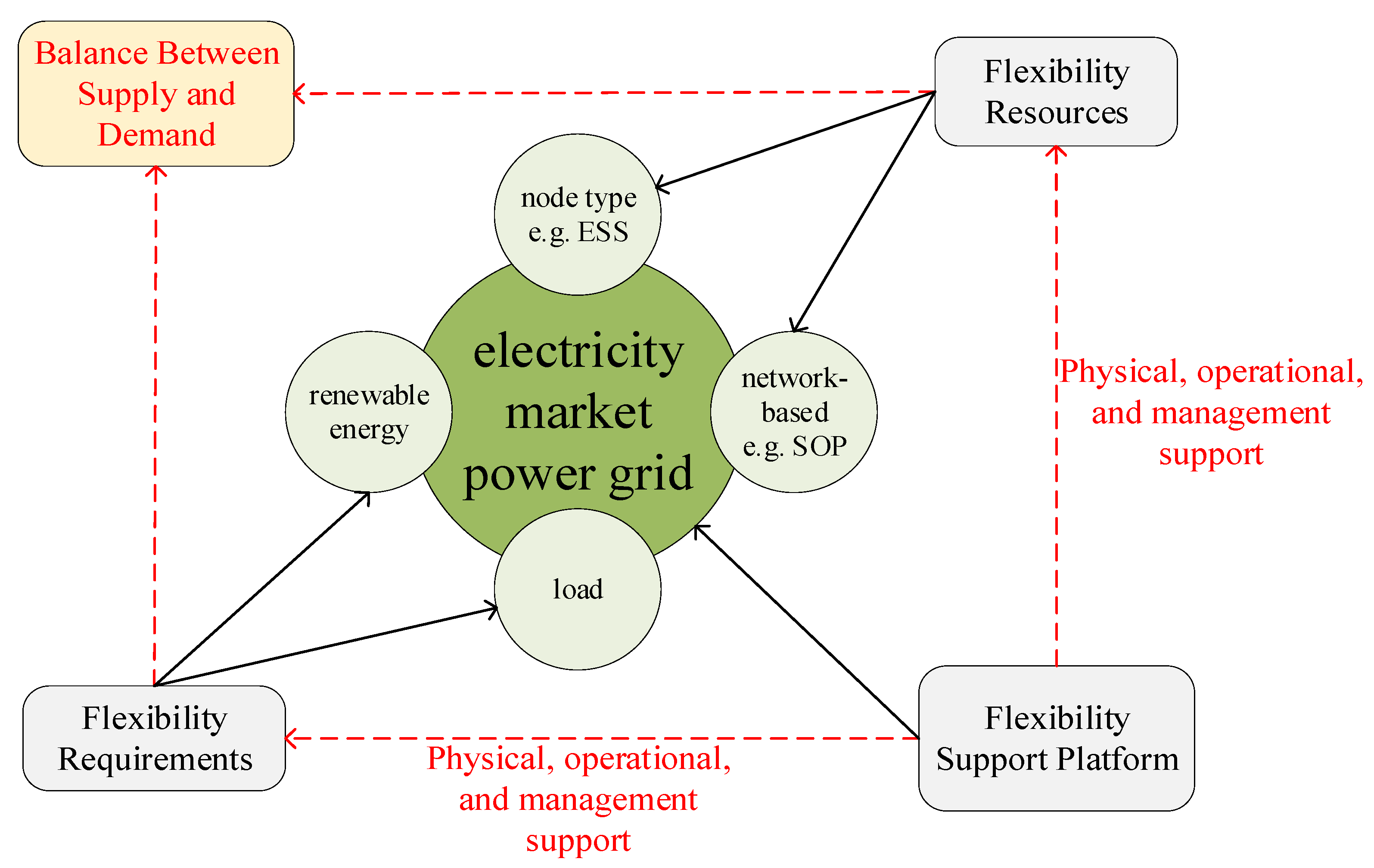
2.1. Distribution Network Flexibility Supply and Demand

The flexibility of ADN is contingent upon the ability to make adjustments within a specified timeframe. This necessitates the effective regulation of both nodal and networked flexibility resources, which must be deployed in a manner that mitigates the inherent volatility and uncertainty of DG. This approach enables balancing of power and supply and demand, thereby facilitating the optimal operating state of the system, which is characterized by both flexibility and economic efficiency. The supply-demand relationship of flexibility is shown in Figure 1.

2.2. Distribution Network Flexibility Resources

Flexibility resources are mainly divided into two categories: networked and nodal. In this paper, networked flexibility resources mainly introduce power electronic devices represented by multiterminal SOP, which realize flexible monitoring and response to the power system through flexible interconnection; nodal flexibility resources mainly introduce ESS, which can independently store and release power.

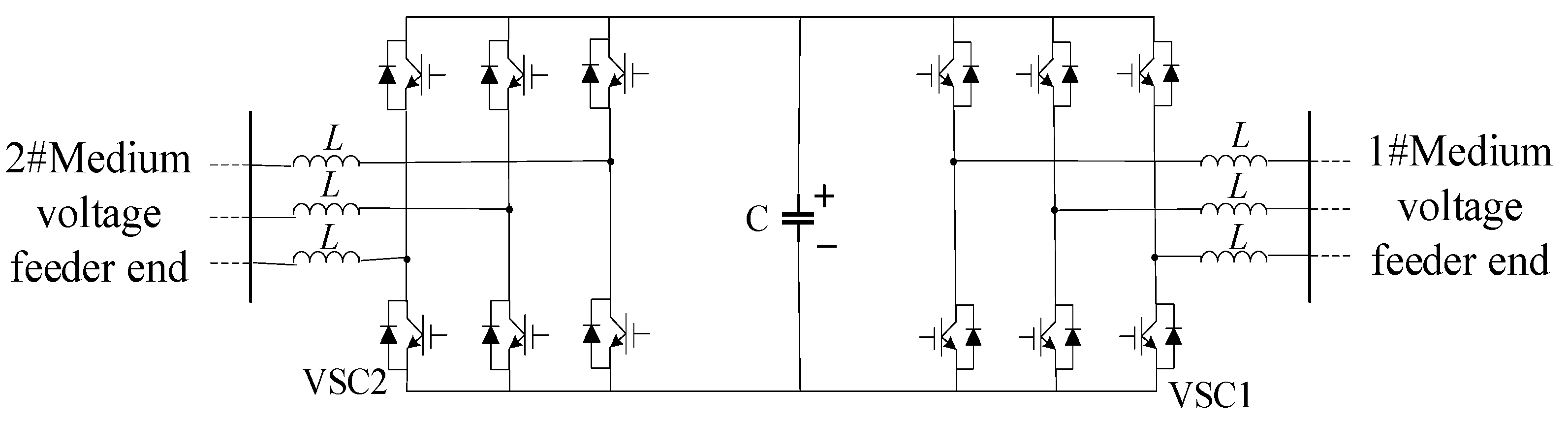
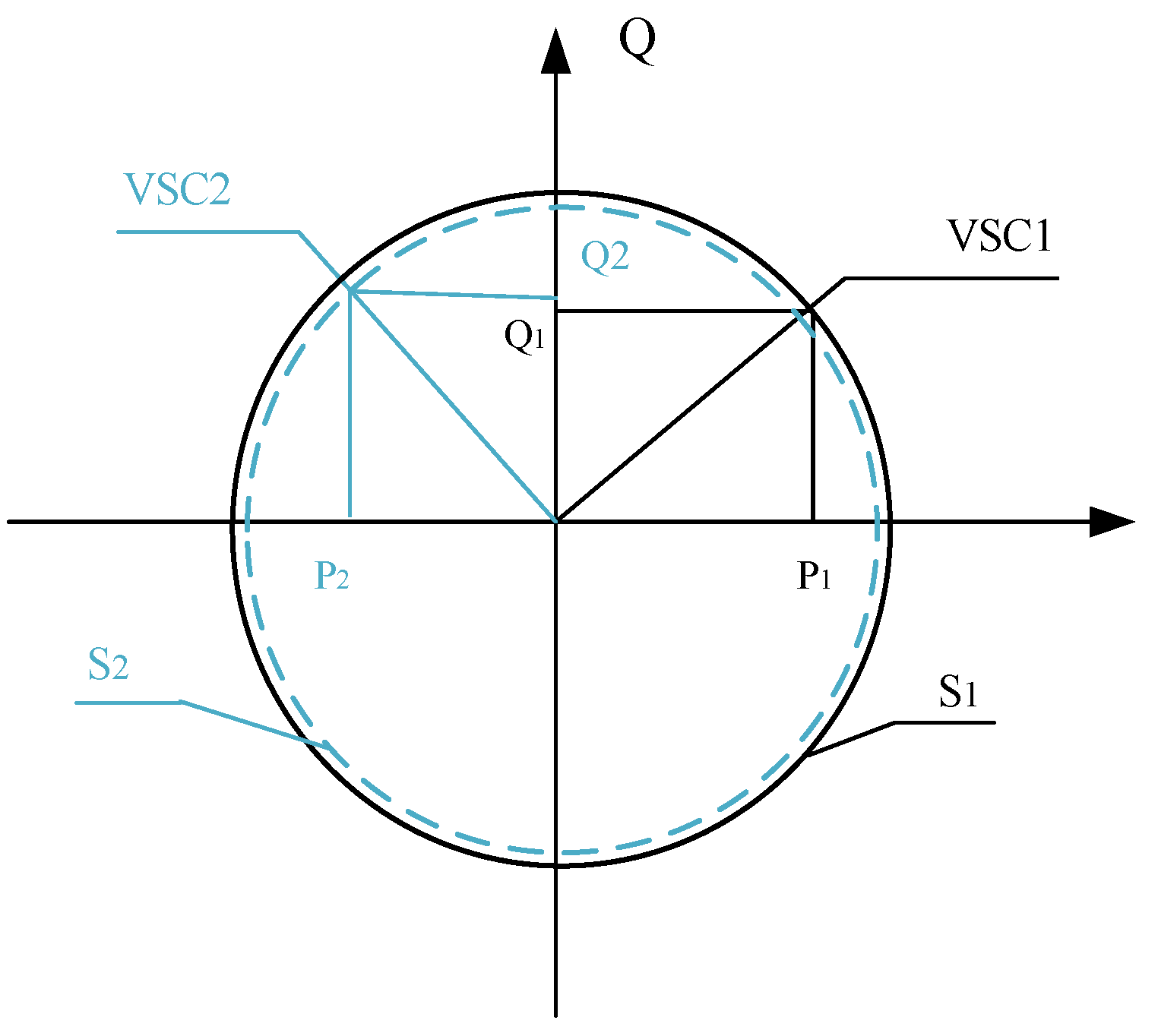
2.2.1. Networked Flexibility Resource

SOP can achieve dynamic active and reactive current control between feeders, balancing load currents and optimizing system voltage distribution, improving the controllability of distribution network currents. At the same time, SOP can be used as a transmission bridge for flexibility, coordinate and deploy flexibility resources, and improve the management efficiency and responsiveness of node-type flexibility resources. This paper presents an illustration of the fundamental configuration of SOP, exemplified by a back-to-back voltage source type converter, as depicted in Figure 2.
When performing active distribution network operation optimization, the variables of SOP are generally selected for their output active and reactive power, and their operating boundaries are shown in Figure 3.
The two ends of the SOP are connected to ADN at nodes i and j. The constraints that should be satisfied for its operation are as follows:
P t , i S O P + P t , j S O P + P t , i j S O P = 0
P t , i j S O P = A i , S O P | P t , i S O P | + A j , S O P | P t , j S O P |
( P t , i S O P ) 2 + ( Q t , i S O P ) 2 S i S O P
( P t , j S O P ) 2 + ( Q t , j S O P ) 2 S j S O P
where i and j are nodes of ADN; t is time period; P t , i S O P and Q t , i S O P are active and reactive power injected by SOP; P t , i j S O P is the active loss of converter at both ends of SOP; Ai,SOP and Aj,SOP are the corresponding loss coefficients; S i S O P and S j S O P are the installed capacities of SOP.

2.2.2. Nodal Flexibility Resource

ESS, as a typical nodal flexibility resource, can realize fast two-way conversion of flexibility through charging and discharging strategies with certain time-scale regulation capabilities. The objective is to achieve a better matching of source and load in ADN, as well as to improve the tidal flow, by low charging and high discharging [19]. The constraints of ESS are as follows:
δ d i s , t + δ c h , t 1
0 P t , i , c E S S δ c h , t P i , max E S S
0 P t , i , d E S S δ d i s , t P i , max E S S
E t + 1 , i E S S = E t , i E S S η c P t , i , c E S S Δ t P t , i , d E S S Δ t η d
E i , 0 E S S = E i , T E S S
E i , min E S S E t , i E S S E i , max E S S
where i represents the node number of the ESS installed in ADN; T and Δt are the number of time periods and the duration of each time period of the operation scenario, respectively, and T = 24 and Δt = 1 h are chosen in this paper; δch,t and δdis,t are state variables in binary numbers, respectively; δch,t/δdis,t = 1 is the charging state, and δch,t/δdis,t = 0 is the discharging state; P t , i , c E S S , P t , i , d E S S , and P i , max E S S are charging and discharging power and the maximum value; E t , i E S S is the charge capacity of ESS; ηc and ηd are charging and discharging efficiencies; E t , 0 E S S and E t , T E S S are the storage capacities of the ESS before and after optimization; E i , max E S S and E i , min E S S are the upper and lower charge limits.

2.3. Distribution Network Flexibility Indicators

Nodal flexibility resources and network flexibility resources cooperate with each other, using the transmission channel provided by the grid structure to complete the different topological combinations of nodal flexibility resources. Under the influence of DG and other random factors, the grid can quickly respond to consume or meet the power in the system.

2.3.1. Traditional Flexibility Indicators

(1)
Net Load Adaptation Ratio
Net Load Adaptation Ratio (NLAR) is the ratio of the dispatchable margin of the nodal flexibility resources to the net load change, which reflects the time attribute characteristic of flexibility. The larger value of the net load adaptation rate indicates that the flexibility resources can satisfy the flexibility demand, and the overall flexibility of ADN is better.
H n e t = 1 T t = 1 T s t + P t , + F S + s t P t , F S | P t + 1 D L P t D L | × 100 %
where Hnet is the net load adaptation rate; s t + and s t denote positive and negative net load changes; P t , + F S and P t , F S are the upward and downward adjustable margins of nodal flexible resources; P t D L is the net load;
(2)
Line Capacity Margin
The line capacity margin indicator, which considers both the structural and the actual state of the line, is defined as the difference between the maximum and actual value of line transmission capacity, expressed as a percentage of the upper maximum value. This indicator reflects the spatial attribute that characterizes flexibility. A greater line capacity margin value indicates that the distribution branch is more resilient to uncertain changes in flexibility demand.
H i j = 1 T × 1 N E t = 1 T i j Ω E ( I i j , max I i j t I i j , max ) × 100 %
where Hij is the line capacity margin; ΩE is the set of branch circuits of ADN; NE is the number of branch circuits of ADN; I i j t is the branch transmission current; Iij,max is the maximum value of transmission current.
The above traditional flexibility indicators are established from the spatiotemporal attributes of flexibility resources, but these two indicators cannot adequately reflect the effect of access to DG on the flexibility of ADN. Consequently, this paper builds indicators from the power side of ADN, whose flexibility is mainly indicated by the admission of DG.

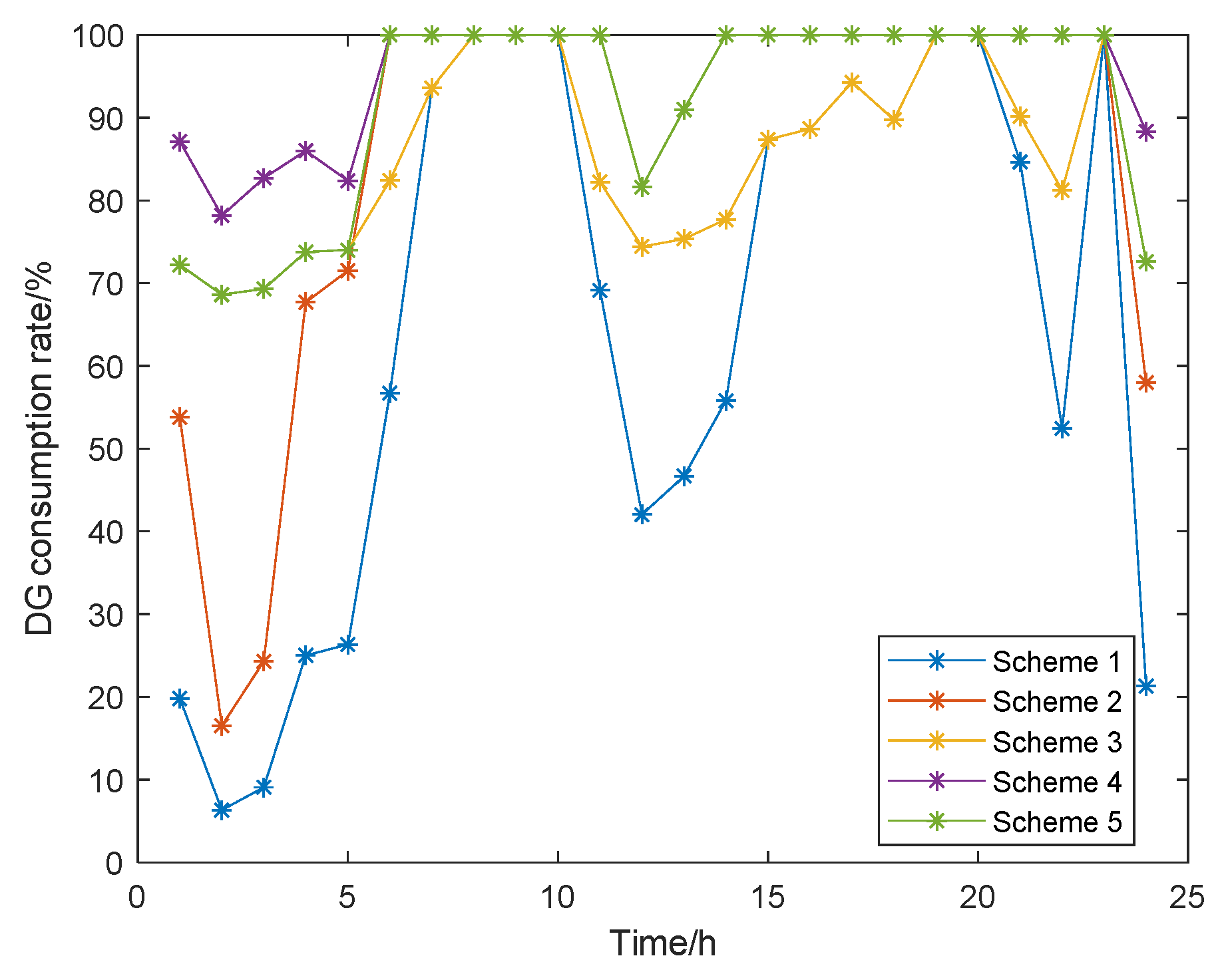
2.3.2. Distributed Generation Consumption Rate

DG consumption rate refers to the proportion of DG systems (e.g., solar, wind, etc.) that are actually consumed or utilized after being connected to the grid. This rate reflects the actual efficiency of the use of DG and is usually expressed as a percentage. Affected by natural conditions and geographical characteristics, China’s new energy distribution is extremely uneven, there is a serious phenomenon of abandonment of wind and solar energy in places where wind and solar energy are abundant, the energy utilization rate is low, and how the grid can consume the output of these new energy sources is an urgent problem to be solved. In this paper, the DG consumption rate is used to measure the ability of ADN to absorb the power from DG.
H x n = 0 T | P G L , t | d t 0 T | P G L , t p r e | d t × 100 %
0 T | P G L , t | d t = 0 T min { | P D G , t p r e | , | P L , t | } d t
where H x n is the rate of renewable energy consumption; PGL,t is the actual power consumption of ADN; P is the output power of DG; PL,t is the load power.
When the load demand is low, to avoid backward transmission, the amount of DG consumed by ADN will be lower than the amount of DG that can be generated, and the consumption rate will be lower than 100%. As the consumption rate approaches 100%, the amount of DG consumed increases, thereby demonstrating the effectiveness of ADN in consuming DG.

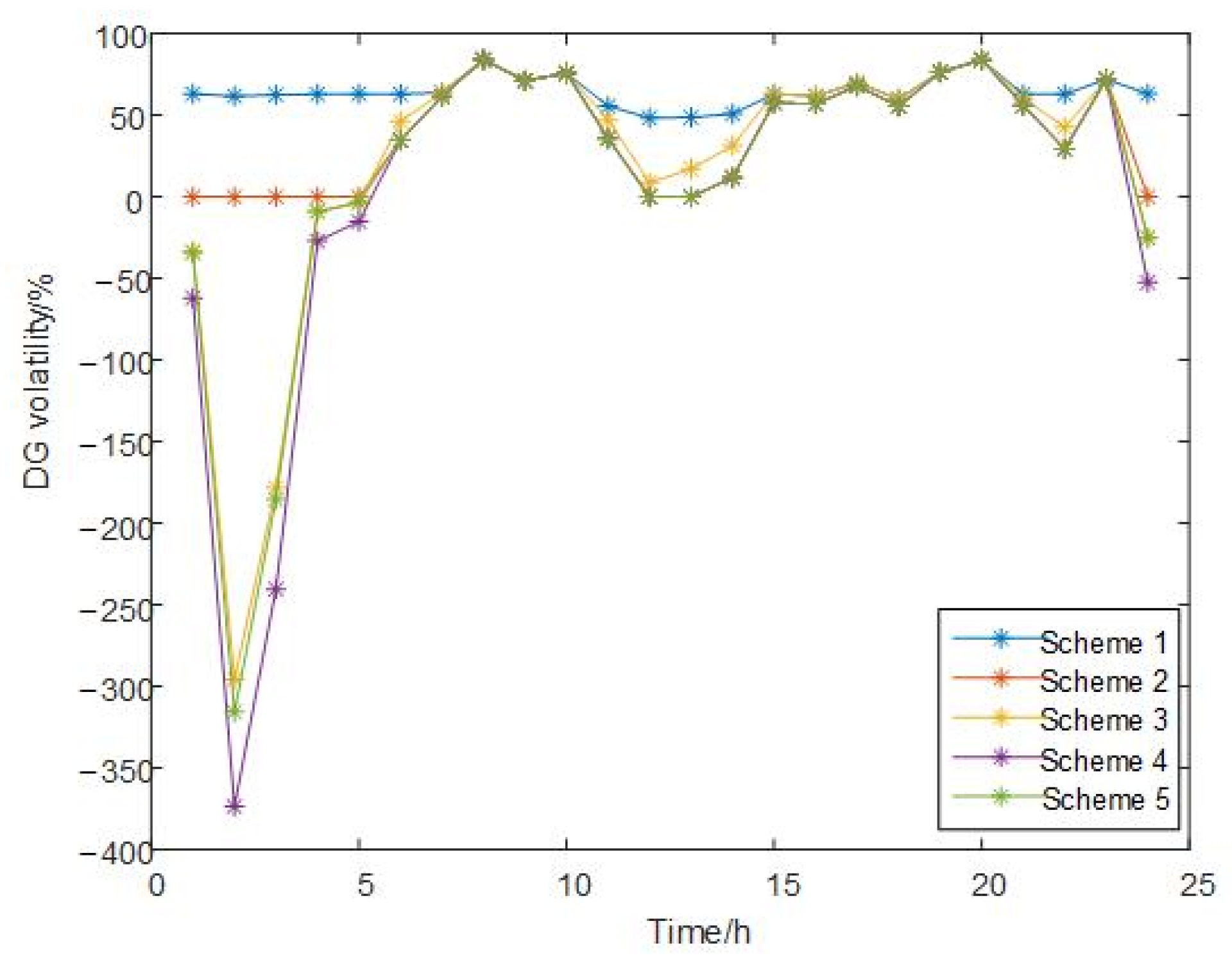
2.3.3. Distributed Generation Volatility

DG volatility refers to the degree of volatility in its power output over a period of time. Since the output of DG is impacted by a variety of factors, including weather conditions, equipment failures, equipment life, and so on. The level of volatility has an important impact on the stable operation and planning of ADN [20].
To reduce the DG volatility, effective planning and management can be implemented to enhance the reliability and quality of the equipment so as to optimize the operation of ADN. Meanwhile, the use of energy storage devices can help balance the volatility and improve the flexibility of the grid. The DG volatility formula is as follows:
H b d = 1 T × 1 n 1 t = 1 T i = 1 n H b d , i t × 100 %
H b d , i t = ( P i t P a v ) 2
where Hbd is DG volatility; n is the number of data spots; H b d t is the volatility of new energy per unit of time; P i t is the practical generating power of DG in the current period; Pav is the average power generation of DG in a period of time.
A higher volatility indicates that the output of DG is more variable and the power quality may be more unstable; conversely, it indicates a more stable generation. DG volatility is usually considered in power system planning or grid connection requirements to facilitate power system scheduling and management.

3. Two-Tier Coordinated Planning of SOP and ESS Considering Flexibility Enhancement of Active Distribution Networks

Considering the impact of strong stochasticity and volatility of WT and PV on coordinated planning, it is necessary to generate a scenario of WT and PV based on C-DCGAN, and then use GA-PSO and cone planning algorithms to carry out two-layer coordinated planning based on the flexibility and economy of ADN using SOP and ESS on the basis of this scenario.

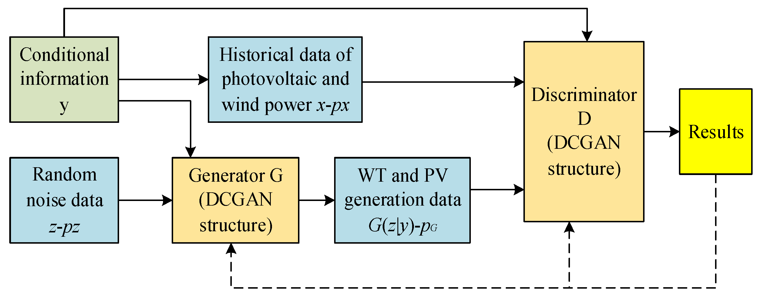
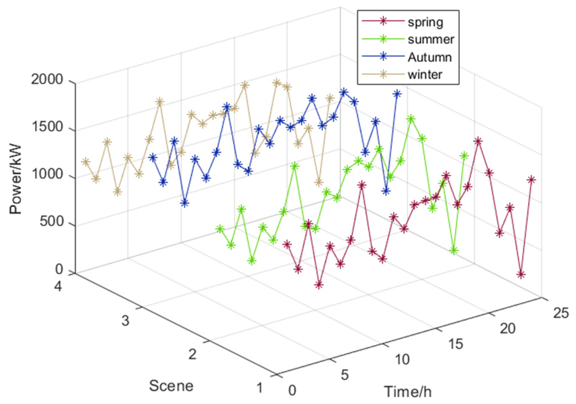
3.1. Scenario Modeling Considering the Uncertainty of Wind Power and Photovoltaic Generation

The ADN mainly consists of photovoltaic generation systems, wind power generation systems, and loads. Among them, the distributed power output is characterized by instability and power volatility [21]. This section presents an analysis of the uncertainty associated with wind and PV output. To address this uncertainty, a scenario generation model for DG output is established using a C-DCGAN based on the Wasserstein distance as the loss function of discriminator D [22].
The conventional methods employed do not adequately take into account the inherent unpredictability of renewable energy sources and the complex inter-relationship between the output characteristics of these sources and the network structure. In comparison with the conventional approach, this methodology assesses the output characteristics of renewable energy sources in terms of their variability and uncertainty. It then designs a network structure that is suitable for the generation of wind scenarios, with the objective of accurately generating wind scenarios that are as close as possible to real-world scenarios.

3.1.1. Using Wasserstein Distance as the Loss Function of Discriminators

The loss function of D in Generative Adversarial Networks (GAN) is equivalent to the JS dispersion, which can result in training difficulties and pattern collapse problems. At the outset of the training process, there is no overlap between the generated and real data samples. Consequently, the loss function is unable to accurately assess the JS distance between the sample distributions. This can result in gradient disappearance during back-propagation, which in turn affects the precision of the scene data generation.
For this reason, the Wasserstein distance is used to replace JS dispersion. The definition is as follows:
W ( p ( x ) , p ( x ) ) = inf Π ( x , x ) d ( x , x ) Π ( d x , d x )
where Π(x, x′) is the joint probability density distribution fulfilling the marginal distributions of p(x) and p(x′); d(x, x′) is the distance measure between scenes.
The Wasserstein distance is a challenging quantity to calculate in a direct manner. Consequently, its Kantorovich–Rubinstein pairwise representation is typically employed for the purpose of describing the discrepancy between the generated sample and the true data:
W ( D ( x ) , D ( G ( z ) ) ) = sup f D L 1 E x P x [ D ( x ) ] E z P z { [ D ( G ( z ) ) ] }
where E(·) is the expected value; D(G(z)) and D(x) are the probabilities that the data G(z) and x is discriminated as true in D; Pz and Px are the distributions of the noisy data z and the scenic data x; ||fD||L ≤ 1 is the 1-Lipschitz continuum that should be satisfied by the discriminator’s loss function, and the upper bound on the absolute value of its derivative is 1.

3.1.2. Conditional Deep Convolutional Generative Adversarial Networks

Deep Convolutional Generative Adversarial Networks (DCGAN) use two convolutional networks to improve the structure of traditional GAN, which improves the stability of the network and accelerates the speed of convergence.
In contrast to GAN, Conditional Generative Adversarial Networks (CGAN) integrate inputs characterized by conditional values within the generator and discriminator. This facilitates the generalization of data samples of the specified type.
This paper presents a novel approach to scene generation that combines the strengths of the previously described methods. The proposed model employs a C-DCGAN to generate realistic images of wind power and PV. Its structure is illustrated in Figure 4.
Specified labels y (e.g., time, weather, etc.) are added to both the generator and the discriminator to DG output scenarios under specific conditions. The objective function of C-DCGAN model is:
min G   max D   V ( D , G ) = E x ~ P x [ D ( x | y ) ] E z ~ P z [ D ( G ( z | y ) ) ] λ E [ D ( ~ ) 1 ] 2
where λE[||▽D(~)|| − 1]2 is the penalty function representing the gradient of the loss function in D; λ represents the penalty coefficient.

3.1.3. Generation of Results for Wind Power and PV Scenarios under Specified Labels

The output data from 288 points of wind power and PV generation for one day are combined and reshaped into a matrix of 24 × 24, which is normalized and used as the input of discriminator D in C-DCGAN. Given the considerable variability in wind power and PV generation across seasons, four seasons were selected as the common labels for wind and solar power generation. This was performed to provide guidance for the generation of combined wind power and PV scenarios. After model training, the generator G generated the scenario of combined wind power and PV, as shown in Figure 5.

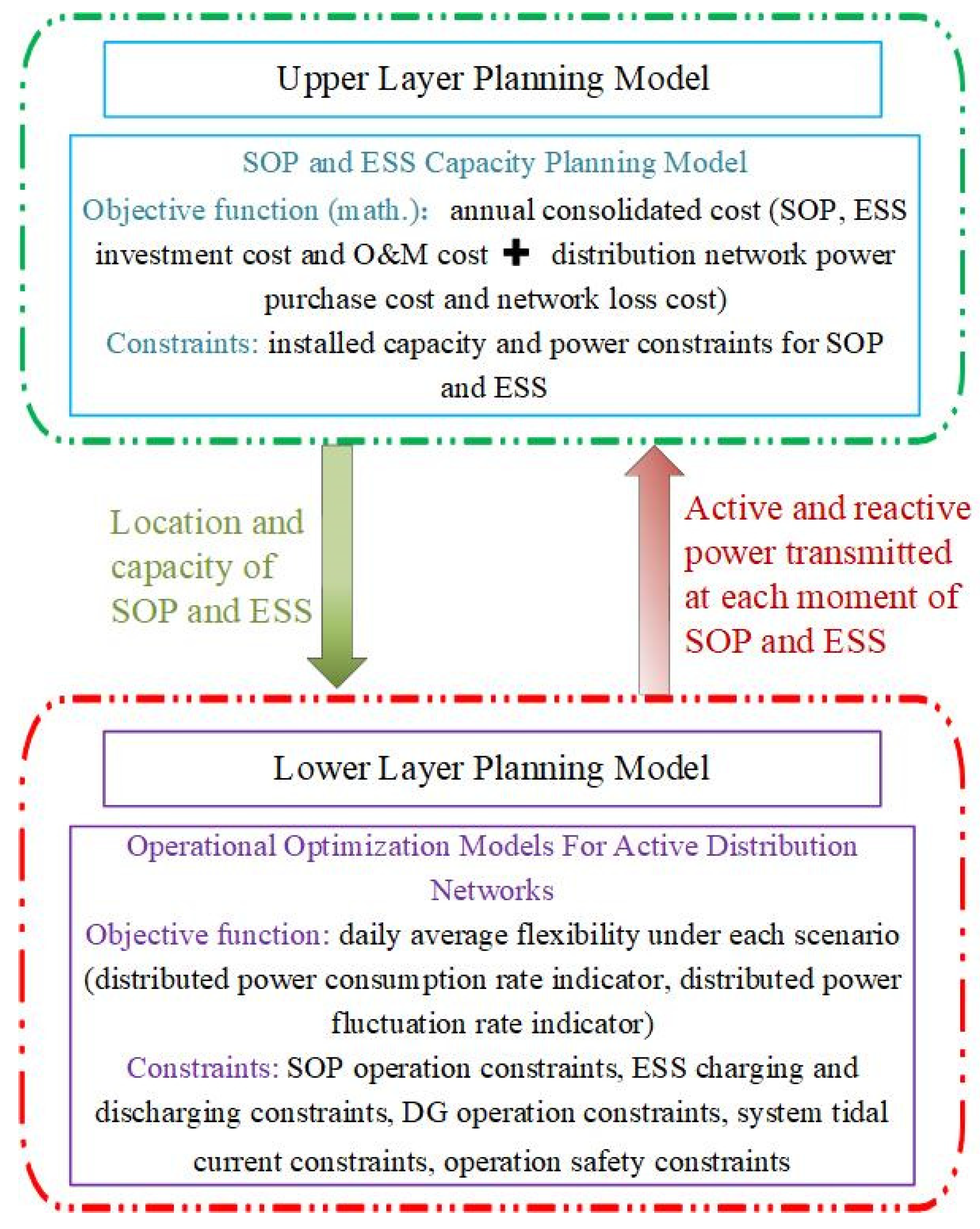
3.2. Two-Layer Planning Model of SOP and ESS

The rapid development of ESS technology and the derivation of SOP has led to the realization that the two can be effectively controlled in a synergistic manner to inhibit the power spatial and temporal fluctuations brought about by DG access to ADN. This paper therefore enhances the DG admittance capacity of ADN through the planning of the two. Since this paper considers both the rational allocation of flexibility resources and the optimal operation of ADN flexibility enhancement, it needs to be decoupled based on the idea of decomposition and coordination. In conclusion, this paper coordinates SOP networked flexibility resources and ESS nodal flexibility resources. It also proposes a two-layer coordinated planning model, as illustrated in Figure 6.
In the planning process, the flexibility of nodes and branches is coordinated in such a way that the ESS and SOP with the optimal capacity are placed in the best position through optimal configuration. This maximizes system flexibility and ensures that there are both sufficient flexibility resources and sufficient flexibility channels in ADN. The upper layer determines the location and capacity of SOP and ESS and transmits this information to the lower layer. The lower layer model is an operational optimization layer that considers the enhancement of ADN flexibility and is used to obtain the optimal operational strategy of ADN under the scenario. The objective of the lower model is to achieve the highest daily average flexibility level, which is comprised of the DG consumption rate index and the DG volatility index. The model transmits power transmitted by SOPs and ESSs at each moment back to the upper layer. Ultimately, the upper and lower layers iteratively optimize each other in order to identify the optimal scheme that simultaneously satisfies both planning and operational requirements.

3.2.1. Upper-Layer Planning Model

The upper layer model is employed to identify the optimal location and capacity of SOP and ESS, with the objective of economic optimization, as reflected by the minimization of the annual integrated cost. The objective function Fup comprises the investment and maintenance cost of SOP and ESS to be planned, with equal annual values, as well as the annual purchase cost and loss cost of ADN.
min F u p = C I S O P + C O M S O P + C I E S S + C O M E S S + C P C + C L
C 1 S O P = λ ( 1 + λ ) y s o p ( 1 + λ ) y s o p 1 i , j Ω b C S O P S i j S O P
C O M S O P = η S O P i , j Ω b S i j S O P
C I E S S = λ ( 1 + λ ) y E S S ( 1 + λ ) y E S S 1 i Ω E S S ( C e E S S E i E S S + C p E S S P i E S S )
C O M E S S = t = 1 T s = 1 S i Ω E S S η E S S | P t , i , s E S S |
C P C = 365 t = 1 T s = 1 S c g P t , s M G
C L = 0 8760 ρ P t L Δ t d t
P t L = s = 1 S ( i j Ω b r i j I s , t , i j 2 + i = 1 N N P s , t , i S O P , L ) × p ( s )
where C I S O P , C O M S O P , C I E S S , and C O M E S S are the investment and maintenance costs of SOP and ESS; CPG is the cost of purchasing power from a higher main network; CL is the annual loss cost of ADN; λ is the discount rate; ySOP is the service life of SOP; CSOP is the SOP unit capacity investment cost; ηSOP is the maintenance cost per unit capacity of SOP; yESS is the economic service life of ESS; C e E S S and C p E S S are the investment cost per unit capacity and power of ESS; ηESS is the maintenance cost per unit capacity of ESS; S is the number of scenarios; cg is the unit price of power purchased from the higher network; P t , s M G is the active power injected into ADN from the superior main network. ρ is the cost of network loss per unit power; P t L is the active power loss of ADN; NN is the number of system nodes; P s , t , i S O P , L is the SOP device loss; Ωb is the set of system branch circuits; p(s) denotes the probability of scenario s.

3.2.2. Lower Layer Planning Model

The lower-layer model is employed to identify the optimal operational strategy for ADN under the specified scenario. The objective is to achieve the highest daily average flexibility level, with the objective function Fdown set as the optimal sum of the daily average flexibility of the distribution system after the assignment, where the flexibility is reflected by the DG volatility and DG consumption rate. The assignment is based on the coefficient of variation, which ensures objectivity.
In accordance with two ADN flexibility evaluation indices introduced in Section 2.3, it can be posited that a higher value of DG consumption rate is indicative of a stronger regulation ability of flexibility resources, a stronger ability to cope with uncertain changes in flexibility demand, and a superior overall flexibility of ADN. Conversely, a lower value of DG volatility is indicative of a superior ability to adapt to uncertainty in flexibility demand. The two indicators are mutually influential, mutually coupled, and mutually acting, and thus the system’s flexibility is determined jointly by the two indicators.
F d o w n = w x n H x n w b d H b d
where wxn and wbd are the weights of DG consumption rate and DG volatility.
In addition, the lower layer needs to satisfy the DG operation constraints, the system trend constraints, and the operation safety constraints besides the operation constraints of SOP and ESS.
(1)
DG operating constraints
0 P s , t , i N D G P s , t , i N D G , p r e
Q i N D G , min Q s , t , i N D G Q i N D G , max
( P s , t , i N D G ) 2 + ( Q s , t , i N D G ) 2 S i N D G
where P s , t , i N D G , P s , t , i N D G , p r e , and Q s , t , i N D G , Q i N D G , max , and Q i N D G , min are the active power and its predicted value and the reactive power and its maximum and minimum value of DG; S i N D G is the capacity of DG.
(2)
System tidal current constraints
i k Ω b P s , t , i k = j i Ω b ( P s , t , j i r j i I s , t , j i 2 ) + P s , t , i
i k Ω b Q s , t , i k = j i Ω b ( Q s , t , j i x j i I s , t , j i 2 ) + Q s , t , i
P s , t , i = P s , t , i N D G + P s , t , i S O P + P s , t , i E S S P s , t , i L O A D
Q s , t , i = Q s , t , i N D G + Q s , t , i S O P + Q s , t , i E S S Q s , t , i L O A D
U s , t , j 2 = U s , t , i 2 2 ( r i j P s , t , i j + x i j Q s , t , i j ) + ( r i j 2 + x i j 2 ) I s , t , i j 2
P s , t , i j 2 + Q s , t , i j 2 = U s , t , i 2 I s , t , i j 2
where Ps,t,ji and Qs,t,ji are the active and reactive power transmitted by branch ij; Ps,t,I and Qs,t,i are the active and reactive power of node; P s , t , i L O A D and Q s , t , i L O A D are the active and reactive power consumed by the load; Us,t,i is the voltage of node i; Is,t,ji is the current flowing in branch ij.
(3)
Operational safety constraints
P s , t , i j 2 + Q s , t , i j 2 = U s , t , i 2 I s , t , i j 2
where U i min and U i max are the lower and upper limits values of node voltage; I i j max is the maximum value of line current.

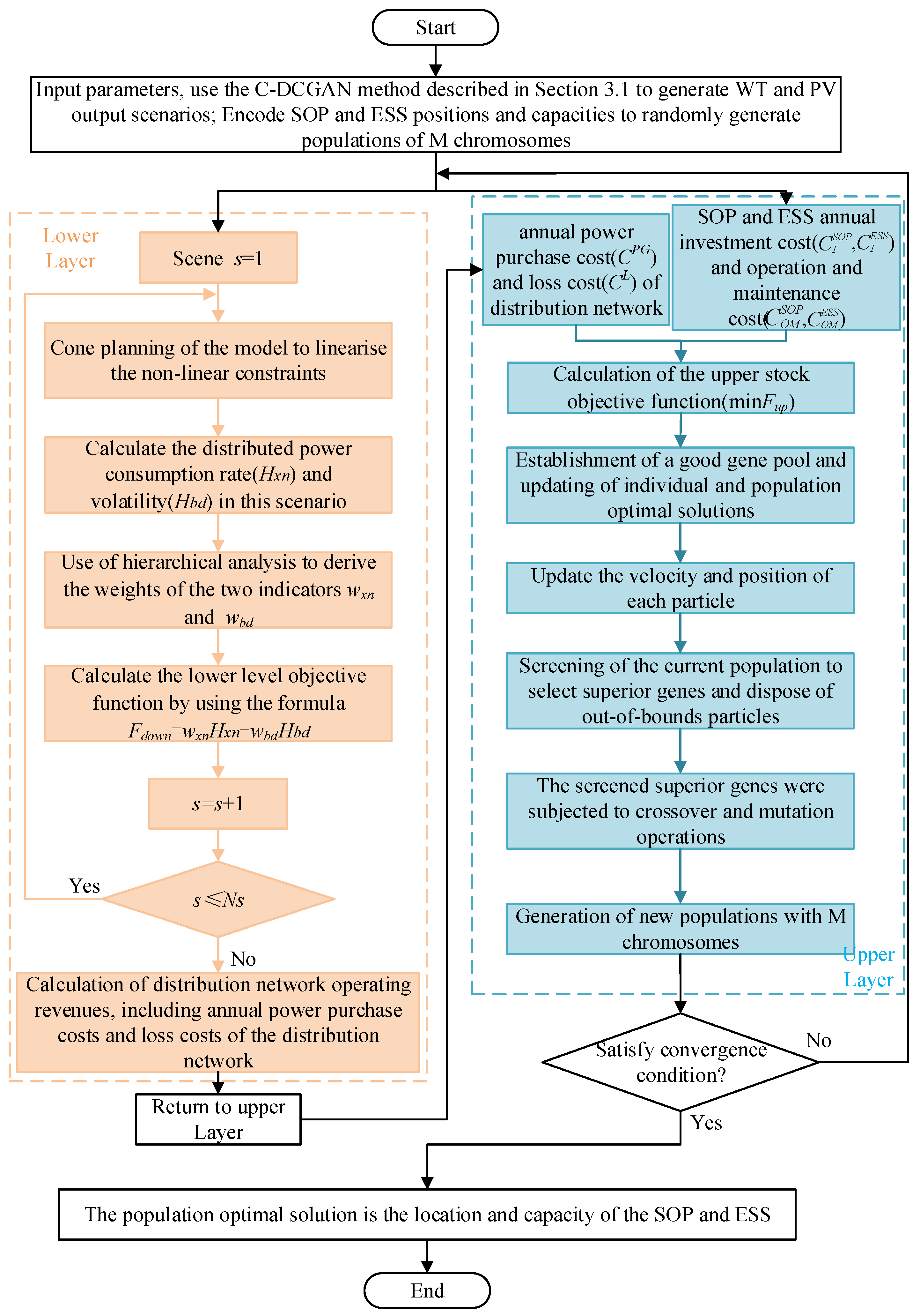
3.3. Model Solving Methods

The two-layer planning models proposed in this paper, namely the SOP and ESS models, belong to the category of large-scale mixed-integer nonlinear planning problems. These problems cannot be solved directly by solvers. Particle Swarm Optimization (PSO) is a simple, fast-converging, local-searching algorithm that has the potential to be easily overfitted. Genetic algorithm (GA) has the advantage of diverse populations and suitability for global search. However, the lack of memory in individuals, the blind and directionless nature of genetic operations, and the long convergence times required present significant challenges. In light of the relative merits and demerits of the two algorithms, an enhanced algorithm, GA-PSO, is put forth for consideration [23]. It has the advantages of PSO and GA at the same time and solves the problems of PSO that easily fall into the local optimum and GA convergence time is long.
Therefore, to decouple the integer variables in the upper layer from the continuous variables in the lower layer, this paper employs GA-PSO and SOCP. The GA-PSO is employed to derive the upper layer SOP and ESS siting and capacity setting scheme. The SCOP is utilized to address the operation optimization problem of the distribution system in the scenario during each iteration of the GA-PSO [24]. The solution flow is depicted in Figure 7.
The particular solution process is as follows:
(1)
The parameters of ADN, PV, wind, and load data are inputted, and typical scenarios are generated according to the C-DCGAN method.
(2)
The SOP and ESS locations and capacities are encoded, and a population of M chromosomes is initially randomly generated.
(3)
The average flexibility of ADN containing SOPs and ESSs is calculated using cone planning.
(4)
The fitness values for each chromosome are calculated.
(5)
The establishment of a robust gene pool, the updating of the historical optimal values of the chromosomes, and the updating of the optimal values of the population are conducted.
(6)
The current population is subjected to selection, gene crossover, and mutation operations, resulting in the generation of a new population of M chromosomes.
(7)
The convergence condition is evaluated. If it is satisfied, the optimal value of the population is output. Otherwise, the process is repeated at step 3.
This paper proposes a two-layer planning model for SOP and ESS, which considers the spatiotemporal regulation characteristics of both. The model aims to reflect the flexibility of the power side of ADN by DG consumption. It is based on the premise that the penetration of distributed power sources is significant.

4. Simulation Analysis

This paper presents an enhanced IEEE 33 power distribution system for the purpose of conducting arithmetic example analysis. The hybrid optimization method proposed in this paper is realized in MATLAB (2023b) by calling the CPLEX algorithm package. Three photovoltaic power supplies and two wind turbines are connected to ADN. The installation locations of PV are nodes 16, 22, and 24, corresponding to an installed capacity of 400, 400, and 400 kW; and the installation locations of the WT are nodes 13 and 20, corresponding to an installed capacity of 1000 and 500 kW. As indicated in the reference [4], the selected nodes for the SOP access points are 6, 16, 22, 24, and 33. These nodes exhibit significant voltage fluctuations. Node 6 is situated in the heavy load branch area, while nodes 16, 22, and 24 are DG access points and are situated near the end of the feeder. Node 33 is situated at the end of the feeder. The specific structure of enhanced IEEE 33 is illustrated in Figure 8. The parameters pertinent to the algorithm are presented in Table 1. In order to validate the joint planning of SOP and ESS that considers the flexibility and economy of ADN, this paper sets up five planning schemes, as shown in Table 2.

4.1. Analysis of the Flexibility of Different Planning Schemes

The simulation of the aforementioned five schemes indicates that the flexibility indicators and the lower objective function of each scheme are calculated by the lower model. The weights wxn and wbd of the two indicators are 0.6 and 0.4, according to the coefficient of variation method. Table 3 presents a comparison of the flexibility indicators of different schemes. A comparison of DG consumption rate indicators is presented in Figure 9. Figure 10 presents a comparison of DG volatility indicators.
As illustrated in Table 3, the DG fluctuation indexes of Schemes 3, 4, and 5 are less pronounced than those of Schemes 1 and 2. This is due to the fact that Schemes 3, 4, and 5 are configured with a nodal flexibility resource, namely an ESS, which transfers active power from time to time through charging and discharging strategies. This enables the reduction of the peak-to-valley difference of the load and the satisfaction of the flexibility demand of the net load. In instances where the power generated by DG exceeds the load, the ESS is capable of storing the surplus energy. Consequently, Figure 10 illustrates that DG volatility may be negative in schemes that incorporate ESS.
The values of the DG consumption rate index and the DG volatility index for Schemes 4 and 5 are greater than those for Schemes 1, 2, and 3. This is due to the fact that Schemes 4 and 5 are configured with network-type flexibility resources. In addition to node-type flexibility resources ESS, SOP can realize fine power control at the feeder level, coordinate various flexible resources, optimally adjust ADN’s current distribution, improve the system’s ability to adapt to the uncertainty of demand, and significantly enhance the ability of DG consumption.

4.2. Economic Analysis of Different Planning Schemes

The preceding five schemes are employed to conduct the simulation, during which the lower model determines the operating cost of ADN in pursuit of optimal daily flexibility. This encompasses the cost of power purchase and network losses from ADN. In contrast, the upper model calculates the annual investment and operating cost of the SOP and the ESS in pursuit of economic optimality. A comparison of the economic indicators of different schemes is presented in Table 4.
A comparison of Scheme 1 with the other four schemes demonstrates that the joint installation of SOP and ESS in ADN can effectively enhance the economic benefits of ADN, thereby corroborating the advantages of the coordinated planning of SOP and ESS. Table 4 illustrates that the economic benefits of Schemes 2–5 are 4.54, 6.6, 10.5, and 11.91. Among these schemes, Scheme 4 is observed to have the greatest impact on economic benefits. Although the installation of SOP and ESS does result in a certain amount of investment costs, the network loss is reduced after the installation of SOP and the peak shaving and valley filling reduces the cost of power purchasing after the installation of ESS. This, in turn, reduces the operation and maintenance cost of ADN and improves ADN benefits accordingly. The revenue of ADN is also improved accordingly.

4.3. Planning Results

From the above results, calculated with the objective of optimal flexibility and economy, the results of the five optimal planning schemes from the simulation are shown in Table 5.
From the aforementioned table, it can be observed that the capacity of Scheme 2 to access SOP is greater than that of Schemes 4 and 5, and the capacity of Scheme 3 to access ESS is greater than that of Schemes 4 and 5. This indicates that the capacity required to access SOP or ESS individually is greater than that required for the synergistic planning of the two. This is due to the fact that both are optimized from a temporal and spatial view of ADN and can be complementary to each other. The capacity of Scheme 4 to access SOP is smaller than that of Scheme 5, but the capacity of Scheme 4 to access ESS is larger than that of Scheme 5. This is due to the fact that Scheme 5 ESS is installed on the DC side of SOP, and the active power will flow through the side of SOP, thereby increasing the access capacity of SOP. However, the ESS is also subjected to the constraints of SOP, and thus the access capacity of ESS becomes smaller.

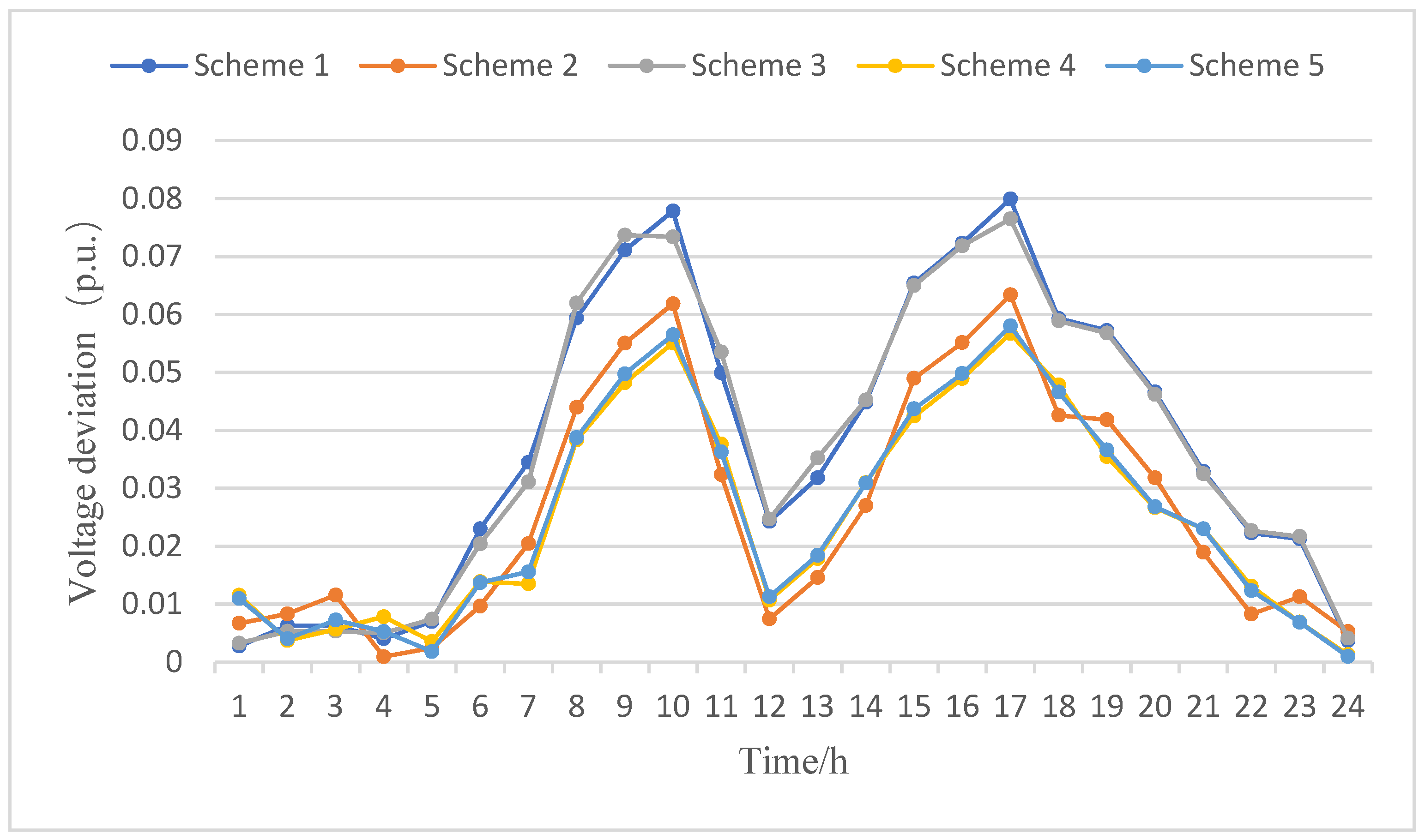
4.4. Analysis of Voltage Quality under Different Planning Schemes

The objective of this analysis is to determine the impact of the planning results derived from the simulation on the improvement of ADN operation, with a focus on voltage quality. To this end, the voltage deviation corresponding to the five planning schemes is presented in Figure 11, which illustrates the deviation in voltage levels. The combined voltage deviation results are presented in Table 6.
As illustrated in the table, despite the objective of optimal flexibility and economy being planned for, Schemes 2–5 all demonstrate varying degrees of improvement in voltage quality in comparison to Scheme 1. Scheme 4 shows the greatest improvement in voltage quality, with 33.7%, 4.6%, 33.5%, and 0.8% improvement over Schemes 1 and 3–5.

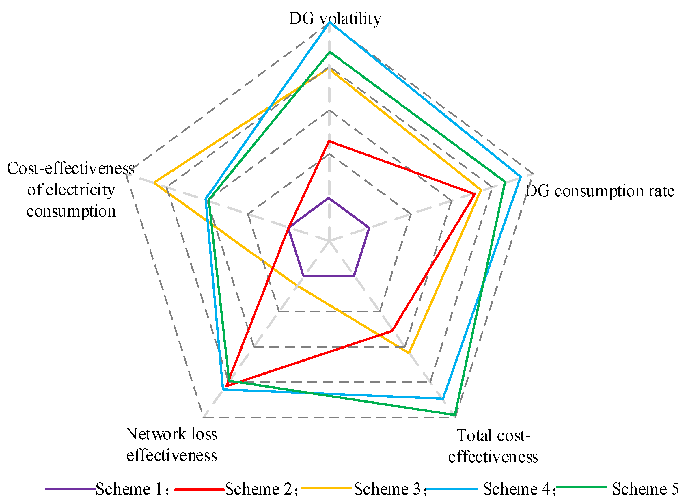
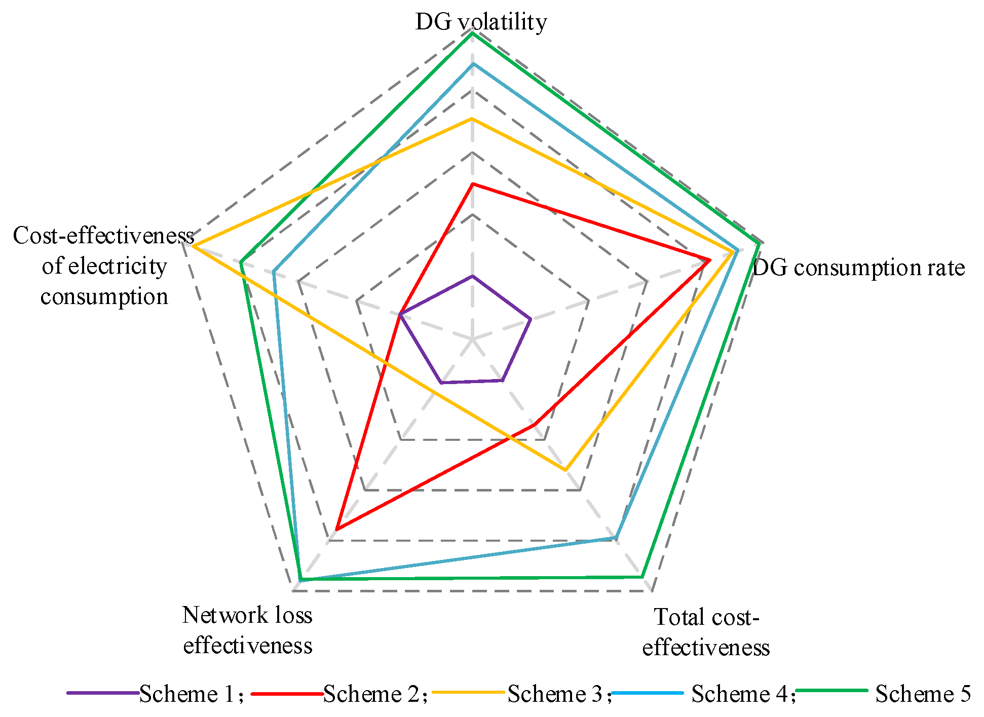
4.5. Comprehensive Benefits Analysis

The preceding economic comparisons and flexibility indicator comparisons have identified the power purchase cost benefit, network loss benefit, and total cost benefit as the most appropriate economic indicators for this analysis. These have been selected in conjunction with two major flexibility indicators. A radar chart of the five major indicators under the five schemes is constructed, as illustrated in Figure 12.
The figure indicates that Schemes 4 and 5 are more economically and flexibly advantageous than Schemes 1 and 2 and 3. This is evidenced by the fact that coordinated planning and operation of the SOP and ESS is more beneficial than accessing the SOP or ESS alone. A comparison of Scheme 4 and Scheme 5 reveals that the total cost of Scheme 5 is 0.36% less than that of Scheme 4. However, the flexibility index is 9.48% lower for Scheme 5. This is due to the fact that the ESS installation location and capacity in E-SOP are constrained by SOP, whereas the ESS in Scheme 4 has the option of selecting a location in close proximity to the distributed power supply, and the capacity can be chosen without being limited by SOP. This can significantly enhance the capability of distributed power consumption. In conclusion, the advantages of coinstallation of SOP and ESS are more evident. Among the five schemes presented in Figure 12, Scheme 4 occupies the largest area of the graph and is therefore the most reasonable.

4.6. Validation of Model Generalizability

In order to verify the universality of the proposed model, a real 10-kV distribution network in a region of China is used as an example. The structure of this distribution network is illustrated in Figure 13, which demonstrates its complex network topology, distributed power access locations, and SOP access points. The PV access capacities are 300 kW and 400 kW, while the WT access capacity is 500 kW. The remaining system parameters are listed in Table 7, including branch impedance and node load. The results of the planning process, as derived from the simulation, are presented in Table 8. The benefits radar chart is illustrated in Figure 14.
The data analysis presented in the above table indicates that the coordinated planning scheme of SOP and ESS reaches the minimum value of the objective function at the upper level and the maximum value at the lower level. This suggests that Scheme 4 has the most superior performance in terms of economy and flexibility. Concurrently, the scheme offers robust backing for practical applications.
As illustrated in the figure, the area of the constituent graphics of the five schemes exhibits variability, with Scheme 4 exhibiting the largest area. This result indicates that Scheme 4 is the most superior in terms of overall performance and reflects its optimal balance in all aspects.
It is noteworthy that the results are in accordance with the simulation outcomes of the IEEE 33-node, which serves to corroborate the universality of the proposed model. This phenomenon indicates that the model is capable of providing effective guidance and support in a variety of network structures and operating conditions. It can be concluded that Scenario 4 is not only applicable to the actual distribution network in the region under consideration, but also provides a valuable reference for the optimization of distribution networks in other regions.

5. Conclusions

This paper presents a novel proposal for the construction of a two-tier planning model, with the objective of achieving both economic efficiency and flexibility in ADN. The model integrates the temporal and spatial trend regulation characteristics of the ESS and SOP, and is verified by an improved IEEE 33 system through arithmetic simulation. The results are as follows:
  • The coordinated planning of SOP and ESS offers superior benefits in terms of enhancing the flexibility and economy of ADN, as well as improving the voltage level of ADN, in comparison to separate individual planning. In comparison to the original plan, the degree of flexibility has been enhanced by 36.92%, the economy of ADN has been improved by 2.58%, and the voltage level has been increased by 33.5%.
  • From the perspective of large-scale penetration of DG, the proposed indicators of DG consumption rate and DG volatility can be employed to comprehensively assess the flexibility of the power side of ADN. Furthermore, they can be utilized as an optimization target to formulate a more reasonable SOP and ESS configuration scheme.
In a subsequent study, social and environmental factors will be taken into account to establish a multiobjective optimization model that simultaneously satisfies the economics and flexibility of the distribution network, as well as the social and environmental benefits, in order to achieve a more comprehensive and reasonable guidance for the siting and sizing of SOP and ESS.

Author Contributions

Conceptualization, J.L. and Y.Z.; methodology, J.L. and C.L.; software, Y.Z. and Z.R.; validation, J.L. and Y.Z.; formal analysis, Y.Z. and Z.R.; investigation, F.Z.; resources, Z.R.; data curation, J.L.; writing—original draft preparation, Y.Z.; writing—review and editing, G.L., J.L., and C.L.; visualization, J.L. and G.L.; supervision, J.L., Z.R., and C.L.; project administration, J.L. and Y.Z.; funding acquisition, J.L. All authors have read and agreed to the published version of the manuscript.

Funding

This research was funded by the National Key Research and Development Program of China and Inner Mongolia Science & Technology Plan under Grant, grant number 2022YFB2403100 and 2022JBGS0043.

Institutional Review Board Statement

Not applicable.

Informed Consent Statement

Not applicable.

Data Availability Statement

The raw data is the IEEE33 node system parameters as shown in Appendix A.

Conflicts of Interest
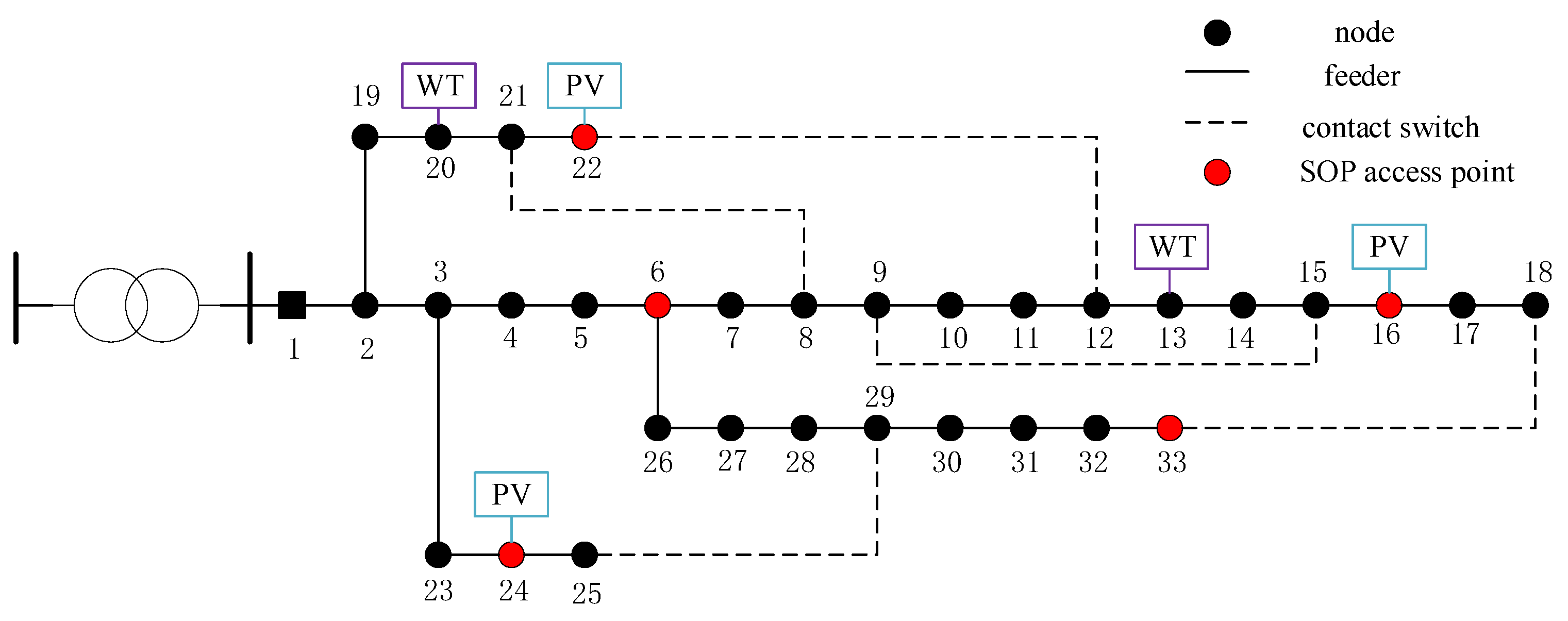
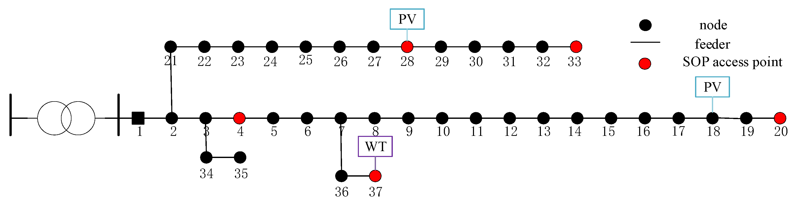
Author Chao Lv was employed by the company Inner Mongolia Power (Group) Co., Ltd., Inner Mongolia Power Research Institute Branch. The remaining authors declare that the re-search was conducted in the absence of any commercial or financial relationships that could be construed as a potential conflict of interest.

Appendix A

Node iNode jBranch ImpedanceNode j LoadNode iNode jBranch ImpedanceNode j Load
120.0922 + j0.0470100 + j6017180.3720 + j0.574090 + j40
230.4930 + j0.251190 + j402190.1640 + j0.156590 + j40
340.3660 + j0.1864120 + j8019201.5042 + j1.355490 + j40
450.3811 + j0.194160 + j3020210.4095 + j0.478490 + j40
560.8190 + j0.707060 + j2021220.7089 + j0.937390 + j40
670.1872 + j0.6188200 + j1003230.4512 + j0.308390 + j50
780.7144 + j0.2351200 + j10023240.8980 + j0.7091420 + j200
891.0300 + j0.740060 + j2024250.8960 + j0.7011420 + j200
9101.0440 + j0.740060 + j206260.2030 + j0.103460 + j25
10110.1966 + j0.065045 + j3026270.2842 + j0.144760 + j25
11120.3744 + j0.123860 + j3527281.0590 + j0.933760 + j20
12131.4680 + j1.155060 + j3528290.8042 + j0.7006120 + j70
13140.5416 + j0.7129120 + j8029300.5075 + j0.2585200 + j600
14150.5910 + j0.526060 + j1030310.9744 + j0.9030150 + j70
15160.7463 + j0.545060 + j2031320.3105 + j0.3619210 + j100
16171.2890 + j1.721060 + j2032330.3410 + j0.536260 + j40
8212 + j2contact switchThe network comprises 32 branch circuits, 5 contact switching branch circuits, and 1 power supply network. The first base voltage is 12.66 kV, the three-phase power quasi-value is 10MVA, and the total load of the network is 5084.26 + 52547.32 kVA.
9152 + j2
12222 + j2
18330.5 + j0.5
25290.5 + j0.5

References

  1. Yang, X.D.; Xu, C.B.; He, H.B.; Yao, W.; Wen, J.; Zhang, Y. Flexibility provisions in active distribution networks with uncertainties. IEEE Trans. Sustain. Energy 2021, 12, 553–567. [Google Scholar] [CrossRef]
  2. Cao, W.; Wu, J.; Jenkins, N.; Wang, C.; Green, T. Benefits analysis of soft open points for electrical distribution network operation. Appl. Energy 2016, 16, 36–47. [Google Scholar] [CrossRef]
  3. Tsai, Y.S.; Chen, C.W.; Kuo, C.C.; Chen, H.C. Design of an Enhanced Dynamic Regulation Controller Considering the State of Charge of Battery Energy Storage Systems. Appl. Sci. 2024, 14, 2155. [Google Scholar] [CrossRef]
  4. Huang, C.; Chen, Y.W.; Mao, Z.P.; Sun, J.; Zha, X. Joint Access Planning for Flexible Multi-state Switching and Distributed Energy Storage System. Power Syst. Autom. 2022, 46, 29–37. [Google Scholar]
  5. Laaksonen, H.; Khajeh, H.; Parthasarathy, C.; Shafie-Khah, M.; Hatziargyriou, N. Towards flexible distribution systems: Future adaptive management schemes. Appl. Sci. 2021, 11, 3709. [Google Scholar] [CrossRef]
  6. Liu, L.; Huang, W.; Chen, Z.; Jiang, Y.; Huang, J.; Chen, F. Novel joint planning of long and short-term energy storage for power systems considering flexibility supply-demand balance. Power Grid Technol. 2024, 1–13. [Google Scholar] [CrossRef]
  7. Cheng, S.; Fu, T.; Li, F.; Gao, X.; Wang, C. Flexible supply-demand co-planning for distribution networks with high penetration of renewable energy. Power Syst. Prot. Control 2023, 51, 1–12. [Google Scholar]
  8. Xiangwu, Y.; Ruojin, L. Flexible Coordination Optimization Scheduling of Active Distribution Network with Smart Load. IEEE Access 2020, 8, 59145–59157. [Google Scholar]
  9. Ma, W.; Gao, H.; Li, H.; Liu, Y.; Liu, J. Flexibility assessment and optimal scheduling model of distribution network considering Soft Open Point. Power Grid Technol. 2019, 43, 3935–3943. [Google Scholar]
  10. Xue, F.; Ma, L.; Zhu, H.; Shi, J.; Qiao, W. Bi-level programming of distributed generations in flexible distribution network with sop optimization. Power Syst. Technol. 2020, 32, 109–115. [Google Scholar]
  11. Zheng, H.; Shi, T. Bilayer optimization of distribution network based on Soft Open Point and reactive power compensation device. Power Syst. Autom. 2019, 43, 117–126. [Google Scholar]
  12. Ji, H.; Wang, C.; Li, P.; Zhao, J.; Song, G.; Wu, J. Quantified flexibility evaluation of soft open points to improve distributed generator penetration in active distribution networks based on difference-of-convex programming. Appl. Energy 2018, 218, 338–348. [Google Scholar] [CrossRef]
  13. Zhu, X.; Lu, G.; Xie, W. Robust planning of distribution network energy storage considering source-network-load flexibility resources. Power Autom. Equip. 2021, 41, 8–16. [Google Scholar]
  14. Sun, W.; Song, H.; Qin, Y.; Heng, L. Optimal allocation of energy storage considering the uncertainty of flexibility supply and demand. Power Grid Technol. 2020, 44, 4486–4497. [Google Scholar]
  15. Guo, Y.; Wu, Q.; Gao, H.; Chen, X.; Østergaard, J.; Xin, H. MPC-based coordinated voltage regulation for distribution networks with distributed generation and energy storage system. IEEE Trans. Sustain. Energy 2019, 10, 1731–1739. [Google Scholar] [CrossRef]
  16. Chongbo, S.; Jingru, L.; Kai, Y. A Joint Optimization Method of Intelligent Soft Open Point and Energy Storage System in Distribution Grid Based on Interval Optimization. High Volt. Eng. 2021, 47, 45–54. [Google Scholar]
  17. Pamshetti, V.B.; Singh, S.P. Coordinated allocation of BESS and SOP in high PV penetrated distribution network incorporating DR and CVR schemes. IEEE Syst. J. 2022, 16, 420–430. [Google Scholar] [CrossRef]
  18. Wang, P.; Li, H.; Zhang, P. Joint Planning of Soft Open Point and Energy Storage in Distribution Networks with Source-Load Imbalance Characteristics. Power Syst. Autom. 2024, 1–15. [Google Scholar]
  19. Kemeng, C.H.; Xi, X.; Peigen, T.I. A comprehensive optimization method for planning and operation of building-integrated photovoltaic storage systems. Chin. J. Electr. Eng. 2023, 43, 5001–5012. [Google Scholar]
  20. He, Y.; Yang, X.; Wu, H.B. Coordinated Planning of Soft Open Point and Energy Storage System for Flexibility Enhancement of New Distribution System. Power Syst. Autom. 2023, 47, 142–150. [Google Scholar]
  21. Mohammedi, R.D.; Kouzou, A.; Mosbah, M.; Souli, A.; Rodriguez, J.; Abdelrahem, M. Allocation and Sizing of DSTATCOM with Renewable Energy Systems and Load Uncertainty Using Enhanced Gray Wolf Optimization. Appl. Sci. 2024, 14, 556. [Google Scholar] [CrossRef]
  22. Zhang, C.; Shao, Z.; Chen, F.; Jiang, C.; Feng, J. A data migration method for new energy generation scenarios based on conditional deep convolutional generative adversarial network. Power Grid Technol. 2022, 46, 2182–2190. [Google Scholar]
  23. Ha, M.P.; Nazari-Heris, M.; Mohammadi-Ivatloo, B.; Seyedi, H. A hybrid genetic particle swarm optimization for distributed generation allocation in power distribution networks. Energy 2020, 209, 118218. [Google Scholar]
  24. Xu, Y.; Han, J.; Yin, Z.; Liu, Q.; Dai, C.; Ji, Z. Voltage and Reactive Power-Optimization Model for Active Distribution Networks Based on Second-Order Cone Algorithm. Computers 2024, 13, 59. [Google Scholar] [CrossRef]
Figure 1. Distribution network flexibility supply and demand.
Applsci 14 08309 g001
Figure 2. Basic structure of SOP.
Applsci 14 08309 g002
Figure 3. Schematic diagram of SOP operation boundary.
Applsci 14 08309 g003
Figure 4. C-DCGAN structure for DG scenario generation.
Applsci 14 08309 g004
Figure 5. Typical scenario of PV and WT combination.
Applsci 14 08309 g005
Figure 6. SOP and ESS two-tier planning modeling framework.
Applsci 14 08309 g006
Figure 7. Flowchart for solving the bilayered regularization model.
Applsci 14 08309 g007
Figure 8. Improved IEEE 33 node structure diagram.
Applsci 14 08309 g008
Figure 9. Comparison of DG consumption rate indicator.
Applsci 14 08309 g009
Figure 10. Comparison of DG volatility indicator.
Applsci 14 08309 g010
Figure 11. Voltage deviation.
Applsci 14 08309 g011
Figure 12. Radar charts for 5 major indicators for 5 schemes.
Applsci 14 08309 g012
Figure 13. Grid structure of the actual distribution network.
Applsci 14 08309 g013
Figure 14. Radar chart for 5 major indicators.
Applsci 14 08309 g014
Table 1. Parameters related to the algorithm.
ParameterValue
Discount rate λ0.08
Useful life of SOP/years20
SOP Investment cost per unit capacity/(dollars/(kV∙A))1500
SOP unit optimized capacity/(kV∙A)10
SOP loss factor0.02
SOP maintenance cost factor0.01
Useful life of ESS/years10
ESS unit capacity cost/(dollars/(kW∙h))400
ESS unit optimized capacity/(kW∙h)100
ESS Charge State Upper and Lower Limits0.9, 0.1
ESS Running Costs/(dollars/(kW·h))0.05
ESS Charge and Discharge Efficiency0.9
ESS Rated Capacity Range/(kW·h)[500, 2000]
Unit network loss cost/(dollars/(kW·h))0.5
Table 2. Planning scheme.
SchemePlanning Content
1No installation of SOP and ESS
2Installation of SOP without ESS
3Installation of ESS without SOP
4Co-installation of SOP and ESS
5Installation of E-SOP
Table 3. Comparison of flexibility of different schemes.
SchemeFlexibility IndicatorsFdown
DG Consumption Rate Hxn/%DG Volatility Hbd/%
165.3754.6817.35
286.0138.8236.08
387.3219.3244.66
494.886.7154.24
591.7914.9449.10
Table 4. Comparison of economies of different schemes.
Scheme C I S O P /Ten Thousand Dollars C O M S O P /Ten Thousand Dollars C I E S S /Ten Thousand Dollars C O M E S S /Ten Thousand DollarsCPC/Ten Thousand DollarsCL/Ten Thousand DollarsFup/Ten Thousand Dollars
10000381.9525.01406.96
24.280.4200381.9515.77402.42
30059.610.30316.2524.20400.36
43.820.3835.770.18341.0215.29396.46
54.130.4129.810.16342.5316.01395.05
Table 5. Planning results of different schemes.
SchemeSOP Planning ResultsESS Planning Results
1----
26-16-33 (840 kVA)--
3--16 (300 kW, 2000 kW∙h)
46-16-33 (750 kVA)16 (200 kW, 1200 kW∙h)
56-16-33 (810 kVA)6-16-33 (150 kW, 1000 kW∙h)
Table 6. Combined voltage deviation results for different planning schemes.
SchemeCombined Voltage Deviation p.u./×10−2
13.77
22.62
33.76
42.50
52.52
Table 7. Parameters of the distribution system.
Node iNode jBranch ImpedanceNode j LoadNode iNode jBranch ImpedanceNode j Load
120.34 + j0.310 + j019200.22 + j0.200 + j0
230.23 + j0.200 + j02210.58 + j0.528.8 + j8.8
340.12 + j0.118.8 + j8.821220.52 + j0.478.8 + j8.8
450.23 + j0.218.8 + j8.822230.41 + j0.378.8 + j8.8
560.27 + j0.2453.25 + j9.7523240.22 + j0.200 + j0
670.22 + j0.190 + j024250.21 + j0.178.8 + j8.8
780.26 + j0.210 + j025260.19 + j0.170 + j0
890.57 + j0.558.8 + j8.826270.21 + j0.190 + j0
9100.46 + j0.4213 + j0.37527280.21 + j0.198.8 + j8.8
10110.45 + j0.420 + j028290.22 + j0.200 + j0
11120.50 + j0.4340.375 + j6.2929300.56 + j0.510 + j0
12130.43 + j0.398.8 + j8.830310.21 + j0.298.8 + j8.8
13140.42 + j0.388.8 + j8.831320.32 + j0.3214.5 + j1
14150.21 + j0.1917.58 + j17.5832330.47 + j0.430 + j0
15160.24 + j0.228.8 + j8.83340.99 + j0.898.8 + j8.8
16170.19 + j0.178.8 + j8.834350.68 + j0.628.8 + j8.8
17180.26 + j0.2313 + j2.257360.19 + j0.178.8 + j8.8
18190.22 + j0.208.92 + j1.37536370.55 + j0.508.8 + j8.8
Table 8. Simulation results.
SchemeSOP Planning ResultsESS Planning ResultsFup /Ten Thousand DollarsFdown
1----295.7314.83
24-20-33 (660 kVA)--292.5633.24
3--16 (330 kW, 1800 kW∙h)289.3242.55
44-20-33 (420 kVA)16 (200 kW, 1300 kW∙h)281.7152.63
54-20-33 (510 kVA)4-20-33 (160 kW, 900 kW∙h)286.4249.47
Disclaimer/Publisher’s Note: The statements, opinions and data contained in all publications are solely those of the individual author(s) and contributor(s) and not of MDPI and/or the editor(s). MDPI and/or the editor(s) disclaim responsibility for any injury to people or property resulting from any ideas, methods, instructions or products referred to in the content.

