Multi-Graph Assessment of Temporal and Extratemporal Lobe Epilepsy in Resting-State fMRI

Abstract

Epilepsy is a common neurological disorder that affects millions of people worldwide, disrupting brain networks and causing recurrent seizures. In this regard, investigating the distinctive characteristics of brain connectivity is crucial to understanding the underlying neural processes of epilepsy. However, the various graph-theory frameworks and different estimation measures may yield significant variability among the results of different studies. On this premise, this study investigates the brain network topological variations between patients with temporal lobe epilepsy (TLE) and extratemporal lobe epilepsy (ETLE) using both directed and undirected network connectivity methods as well as different graph-theory metrics. Our results reveal distinct topological differences in connectivity graphs between the two epilepsy groups, with TLE patients displaying more disassortative graphs at lower density levels compared to ETLE patients. Moreover, we highlight the variations in the hub regions across different network metrics, underscoring the importance of considering various centrality measures for a comprehensive understanding of brain network dynamics in epilepsy. Our findings suggest that the differences in brain network organization between TLE and ETLE patients could be attributed to the unique characteristics of each epilepsy type, offering insights into potential biomarkers for type-specific epilepsy diagnosis and treatment.

1. Introduction

Epilepsy is one of the most common neurological disorders, affecting around 50 million people worldwide [1] and characterized by recurrent, unprovoked seizures (elicited by sudden, abnormal bursts of neural activity in the brain) that can result in alterations in behavior, motor functions, sensory perceptions, or levels of consciousness [2]. Despite multiple antiepileptic drugs, over 30% of epilepsy patients continue to experience seizures and report lower quality of life (QoL) [3,4,5]. In children, epilepsy surgery has shown a higher rate of seizure freedom compared to pharmacological treatment [6]. On the other hand, although surgical resection can improve seizure freedom, it carries cognitive impairment risks [6,7]. In this regard, the identification of brain areas involved in epilepsy is particularly important due to their unique characteristics and challenges in each individual patient [8]. Accurate non-invasive localization can improve surgical outcomes while preserving cognitive functions, allowing more patients to successfully undergo epilepsy surgery [9,10].

Although several modalities have been implemented in epilepsy research and clinical management, functional magnetic resonance imaging (fMRI) can optimize spatial resolution, providing insights into brain activity and seizure propagation in the brain [11]. As such, by utilizing the blood oxygenation level-dependent (BOLD) signal, fMRI can track how the brain reorganizes itself in response to seizures or treatments.

The recent review by Feng et al. [12] presents a comprehensive overview of biomarkers related to pediatric epilepsy, including 62 studies that exclusively utilized fMRI data. According to the review, integrating fMRI analysis with graph theory provides a robust framework for enhancing predictions related to cognitive performance, assessing surgical outcomes, and evaluating symptom severity in focal epilepsy. In fact, neural plasticity can elucidate the brain’s ability to adapt and reorganize itself, both functionally and structurally [13]. Furthermore, chronic seizures can lead to changes in functional neural networks, making certain regions more prone to generating and spreading seizures.

On this premise, functional connectivity (FC) analysis allows the brain to be represented as a graph, where edges can represent the temporal dependencies of signals from the nodes, which can be the anatomical brain regions [14]. In this network, different brain regions have specialized functions and work together to perform higher cognitive functions [15]. Epilepsy has been characterized as a brain network disorder since the seizures not only affect the epileptogenic regions but can also spread to anatomically distant brain regions [16]. From this standpoint, multiple studies underline the importance of the resting-state fMRI (rs-fMRI) FC analysis in decision-making about epilepsy surgery [17,18]. Foit et al. [18] suggested that connectivity-based biomarkers could enhance preoperative evaluation, emphasizing the role of FC in predicting cognitive outcomes post-epilepsy surgery and in localizing the epileptogenic zone. Boerwinkle et al. [17] demonstrated that incorporating rs-fMRI connectivity into the presurgical evaluation resulted in a 50% increase in positive decisions for surgery. In this regard, the incorporation of graph-theory metrics can increase our comprehension of how distant brain regions contribute to information processing, introducing new biomarkers associated with brain network disorders such as epilepsy [19].

This aspect has sprung an increase in research attention towards the topological features that distinguish the epileptic brain network from the healthy one. Specifically, since epilepsy often involves abnormal connectivity patterns in the brain, network metrics, such as global efficiency, clustering coefficients, and path lengths, can highlight changes in brain connectivity over time, providing insights into the neural disruptions, aiding in diagnosis, treatment or surgical planning, and understanding the underlying mechanisms of epilepsy [19,20]. The use of graph-theory fMRI biomarkers is especially important in clinical applications [21]. For instance, the study of Doucet et al. [22] displays the value of graph theoretical features in the prediction of neurocognitive outcomes through the presurgical evaluation of TLE patients, proposing a model of three topological features (distance, local efficiency, and participation) capable of explaining more than 68% of the variance observed in the neurocognitive functions. Moreover, longer path lengths (indicating a lower global efficiency) in the graphs of patients with temporal lobe epilepsy (TLE) compared to controls are frequently observed [23,24,25,26,27,28].

Most notably, graph-theory metrics help in characterizing the overall architecture of brain networks, identifying hubs (the regions that have a key role in the information flow since they facilitate communication between other regions), and understanding how different regions interact. In fact, hub-related analysis can reflect adaptive changes in network connectivity, demonstrating distinct functional or structural characteristics in individuals with neurological disorders [29]. In this context, numerous studies emphasize the significance of hub reorganization in epilepsy, highlighting its role as a critical biomarker associated with patients’ cognitive impairments. A meta-analysis of Crossley et al. [30] concludes that the hub regions are prone to turning into lesions in a variety of brain disorders, and their increased biological cost is combined with higher vulnerability compared to the non-hub regions. Interestingly, they report significantly increased values of degree centrality in the lesion voxels compared to the non-lesion voxels in 9 of the 26 disorders analyzed, where 3 of them include different types of epilepsy (right and left TLE, juvenile myoclonic epilepsy). Regarding TLE patients, the study of Bernhardt et al. [23] reports different hub organization in patients compared to controls, with most of the TLE hubs localized in the paralimbic and the temporal lobe. Another relevant study also presented a shift in the hub localization of TLE patients, with the 98% of the hub regions of the right TLE group located in the contralateral hemisphere to the epilepsy onset [31]. Moreover, the study by Royer et al. [32] summarizes the utility of hub-mapping analysis in the diagnosis, the formation of a treatment plan, and the presurgical evaluation of patients with epilepsy, as well as highlighting the necessity for further investigation of the hub-mapping techniques.

There is a need for extensive validation and refinement of our understanding of brain reorganization in epilepsy, and for accurately identifying hub nodes and predicting the spread of epileptic discharge in the individual patient’s brain. However, most studies employ only degree centrality to identify hub nodes, neglecting other measures that consider the distance between regions or their ability to facilitate connections. Furthermore, most relevant research analyzes average graphs constructed from mean connectivity values within each group, thus disregarding individual-specific brain networks.

In this study, we aim to address these constraints by evaluating the importance of the regions of interest (ROIs), employing four centrality measures for the hub definition in three different connectivity techniques. Moreover, instead of analyzing the mean brain network, we analyze the hubs of each subject separately and then create the hub probability based on their presence within each group, minimizing the averaging bias. Specifically, we introduce a methodological framework to do the following:

• Explore the brain reorganization characteristics and their differences between epileptic patients and healthy controls.
• Reveal the hub regions, utilizing different brain connectivity methods and assessing the centrality measures to quantify the importance of a node.
• Uncover the regional alterations in hub probability, identifying the ROIs that play a critical role in both healthy individuals and TLE and/or ETLE patients.

For this purpose, we employ three different connectivity techniques (Pearson correlation, mutual information (MI), and Granger causality) to construct graphs for each subject among TLE and ETLE patients as well as healthy controls. Subsequently, we compare the global centralization features between all subjects and groups at different density level thresholds. Further, we calculate the hub probability of each ROI for each group and assess their differences to offer a comprehensive understanding of the areas controlling the information flow in each type of epilepsy and give prominence to the hub reorganization as a possible biomarker to predict network restructuring in epilepsy.

2. Materials and Methods

2.1. Subjects

Data were gathered retrospectively and include resting-state fMRI recordings from 65 individuals, 44 of which were epilepsy patients (21 females), and 21 healthy controls (12 females). Subsequently, the patient group dataset was divided into temporal lobe epilepsy (TLE—28 subjects, 12 females, mean age 28.4 ± 8.9) and extratemporal lobe epilepsy (ETLE—16 subjects, 9 females, mean age 21.3 ± 6.4) (

Table 1. Demographic and clinical characteristics of healthy controls.

Characteristics
Number of Individuals	21
Female, N (%)	12 (57.1)
Age, mean in years (std, range)	31.6 (7.4, 18–44)
Handedness: left, N (%)	0 (0)
Handedness: right, N (%)	20 (100)
Language Lateralization: left, N (%)	19 (95)
Language Lateralization: right, N (%)	1 (5)

and

Table 2. Demographic and clinical characteristics of patient groups.

Characteristics	TLE	ETLE
Number of Individuals	28	16
Age, mean in years (range)	28.4 ± 8.9 (14–41) *, **	21.3 ± 6.4 (13–40) **
Age of seizure onset,	17.1 ± 12.1 (0.2–39) **	2.5–39
Affected Hemisphere
Left, N (%)	19 (67.9)	11 (68.75)
Right, N (%)	7 (25)	5 (31.25)
Bilateral, N (%)	2 (7.1)	0 (0)
Pathology
Grade I astrocytoma	3 (10.7)	2 (12.5)
Ganglioglioma	2 (7.1)	0 (0)
Gliosis	0 (0)	1 (6.25)
MTS	5 (17.9)	0 (0)
Meningioma	0 (0)	1 (6.25)
DNET	3 (10.7)	1 (6.25)
FCD	3 (10.7)	3 (18.75)
unknown	12 (42.9)	5 (31.25)

Note: Asterisk (*) denotes a statistical difference with the control group (p < 0.05); Double asterisk (**) denotes a statistical difference between the patient groups (p < 0.05); MTS: Medial Temporal Sclerosis; DNET: Dysembryoblastic Neuroepithelial Tumor; FCD: Focal Cortical Dysplasia.

). The control group (mean age 31.6 years (±7.4)) was screened prior to data acquisition to ensure no history of neurological diseases or drug abuse, and each reported normal or corrected-to-normal vision and right hand as dominant [33]. Patient group inclusion criteria were as follows: (1) epilepsy patient, either temporal epilepsy or extratemporal epilepsy, (2) ability to complete all necessary recordings, (3) MRI negative or small lesion that does not interfere with the brain architecture/structures, and (4) no anesthesia during the fMRI acquisition. Assignment to either the temporal (TLE) or the extratemporal (ETLE) group was determined following a comprehensive presurgical evaluation protocol in the “St. Luke’s” Epilepsy Center on the basis of localizing information obtained through prolonged Video-EEG monitoring, structural MRI, and in selected cases, additional studies such as EEG-FMRI and PET. Data recording was performed in accordance with the Declaration of Helsinki, while the study was approved by the Institution’s Review Board (3 April 2024). Prior to all processing and analysis procedures, data anonymization was performed.

2.2. Data Acquisition

All fMRI recordings were performed at “St. Luke’s” Hospital, Thessaloniki, Greece. Since bias can be introduced if different instrumentation is used [34], all data acquisition utilized the same scanner, i.e., a 1.5T AVANTO FIT MRI scanner with a standard Siemens 20-channel head coil. The MRI protocol included(a) resting-state fMRI, 2 × 2 × 2 mm³ voxel size, TR 1700 ms, TE 50 ms, 530 volumes, 15 min, (b) gradient field map, 2 × 2 × 2 mm³ voxel size, 228 × 228 × 170 mm³ field of view, 4.76 ms and 9.52 ms the two echo times, (c) T1 MPRAGE, 1 × 1 × 1 mm³ voxel size, 250 × 250 × 192 mm³ field of view, (d) T2 FLAIR, 1 × 1 × 1 mm³ voxel size, 260 × 252 × 176 mm³ field of view. All resting-state fMRI were acquired at the beginning of each session. Subjects were instructed to keep their eyes closed throughout the acquisition while trying not to fall asleep. Pneumatic headphones were used to insulate from the scanner noises, but no music or other audio was playing during fMRI acquisition. More details of the data acquisition procedures can be found in [33].

2.3. Preprocessing

The FMRIB’s Software Library (FSL; v 6.0.1; https://www.fMRIb.ox.ac.uk/fsl; accessed on 15 January 2024) was utilized for the preprocessing pipeline of fMRI data [35]. Gradient field maps were utilized to estimate the scanner inhomogeneities for data correction and better registration procedures. The effective echo spacing of the fMRI data was at 0.78 ms. The preprocessing pipeline included brain extraction, motion correction via linear registration with 6 DOF to the middle fMRI volume of the acquisition, spatial smoothing with a kernel of 4 mm FWHM, grand mean intensity normalization, and a high pass filter at 100 s. Registration was performed from the fMRI template image to the T1 image with the BBR algorithm and inverted to apply the transformation to the label image and capture the time series of each region in the fMRI space to avoid unnecessary interpolations [36,37]. Afterwards, independent component analysis was performed for each session and the components related to any artifact were manually recognized and regressed out of the signal for the subsequent analysis [38,39]. Registration to a template was not performed, as the time series were extracted to the fMRI space for each subject.

2.4. Segmentation and Time Series Extraction

The atlas utilized in the current study is the Destrieux atlas [40], as they were parcellated from FreeSurfer [41]. For the segmentation, both T1 isotropic and T2 FLAIR images were utilized, with a total of 160 regions being parcellated into cortical and subcortical regions (the names and abbreviations of the brain regions can be found in Appendix A). The mean value of each region in each timepoint was calculated to create the time series of the regions for each subject from the preprocessed signal.

2.5. Brain Connectivity Estimation

For each subject, the temporal dependencies between the BOLD time series extracted from the ROIs of the Destrieux atlas were estimated using three connectivity methods: the Pearson correlation, the mutual information (MI), and the Granger causality. The mathematical formulas for each method can be found in Appendix B. Each method output was a connectivity matrix with size 160 × 160. The corresponding graphs were constructed at a subject level with 160 nodes denoting the ROIs used for the analysis, and the edges between those ROIs represented the strength of their dependence, expressed by the values of the connectivity matrices. The correlation matrices corresponding to the Pearson correlation [42] and the mutual information (MI) [43] are undirected (symmetric), while the causation matrix corresponding to the Granger causality [44] is directed (asymmetric).

To ensure stability of the graph-theory metrics, the same number of edges were taken into account, applying a proportional threshold on the edges of the graph to preserve a specific density level [45]. Specifically, we define as density level the percentage of the edges/connections preserved in the final graph, while all other edges were set to 0. In this study, ten (10) density levels were utilized, from 5% to 50% with a step of 5%, resulting in the construction of 30 graphs in total for each subject (10 of each density level × 3 connectivity metrics × 65 subjects = 1950 graphs). A schematic of the applied framework is presented in Figure 1.

2.6. Global Network Analysis

Accordingly, each graph was investigated for its topological characteristic via the graph metrics of (i) global assortativity, (ii) global efficiency, (iii) global (mean) clustering coefficient, and (iv) number of components. The definitions of the aforementioned global topological features are included in

Table 3. Definitions of the global topological features.

Features	Description
Global assortativity	Assesses the similarity of the nodes connected in the graph, concerning their degree centrality. High positive values of assortativity indicate that the nodes tend to connect with nodes with similar centrality degrees. Negative values indicate that the hubs of the network tend to connect with low-degree nodes [46].
Global efficiency	Measures how easily information can travel between any pair of nodes. High values indicate a more integrated and well-connected network. Lower global efficiency suggests a network where information transfer is less efficient, indicating potential disruptions or fragmentation in network connectivity [47]. Mathematically, it can be formed as follows: $${\mathrm{E}}_{\mathrm{G}\mathrm{l}\mathrm{o}\mathrm{b}\mathrm{a}\mathrm{l}}={\displaystyle \frac{1}{\mathrm{N}(\mathrm{N}-1)}}\sum _{\mathrm{i}\ne \mathrm{j}\in \mathrm{G}}{\displaystyle \frac{1}{{\mathrm{d}}_{\mathrm{i}\mathrm{j}}}}$$ $\mathrm{where} {\mathrm{d}}_{\mathrm{i}\mathrm{j}}$ is the shortest path length that connects the nodes i and j in the graph.
Mean clustering coefficient	Quantifies the degree to which nodes tend to cluster together. High mean clustering coefficient values suggest that there are many localized clusters of interconnected brain regions, which might be indicative of specialized functional modules within the brain [48]. Low values of the mean clustering coefficient indicate that the graph cannot be divided into clusters, and most of its nodes participate in closed triangles [49]. The mean clustering coefficient can be calculated as the average of the nodal clustering coefficient from all the nodes in the graph: $${\mathrm{C}\mathrm{C}}_{\mathrm{G}\mathrm{l}\mathrm{o}\mathrm{b}\mathrm{a}\mathrm{l}}={\displaystyle \frac{1}{\mathrm{N}}}\sum _{\mathrm{i}\in \mathrm{G}}{\mathrm{c}}_{\mathrm{i}}$$ ${\mathrm{c}}_{\mathrm{i}}$ is the clustering coefficient of the node i, which is calculated according to the following formula: $${\mathrm{c}}_{\mathrm{i}}={\displaystyle \frac{2{\mathrm{T}}_{\mathrm{i}}}{{\mathrm{d}}_{\mathrm{i}}({\mathrm{d}}_{\mathrm{i}}-1)}}$$ ${\mathrm{T}}_{\mathrm{i}}$ denotes the number of triangles that include the node i, and ${\mathrm{d}}_{\mathrm{i}}$ is the degree of this node.
Number of components	Evaluates the maximal connected subgraphs within the entire network. A graph with only one component is fully connected, while a graph with multiple components is disconnected or has distinct clusters.

. Those global features are calculated for each of the 3 × 10 = 30 graphs corresponding to each subject (3 types of graphs—Pearson, MI and Granger, and 10 density levels) resulting in 120 total features (30 graphs and four global topological metrics) for each subject. For each of the global topological features, an ANOVA test among the groups was implemented (p < 0.05 FDR corrected). Tukey–Kramer post hoc test was implemented to infer the statistically significant changes between each pair of groups (p < 0.05).

2.7. Hub-Related Analysis

2.7.1. Probability Distribution in Regions of Interest

Following the global topological characteristics, we aimed to identify the important brain areas (hubs) associated with TLE and ETLE. To do so, we focused on various centrality measures which quantify the importance of each node in the graph (

Table 4. Definitions of the nodal topological features.

Measures	Description
Degree centrality	Measures the number of edges starting from the region. For the directed graph of Granger causality, we used the sum of the in-degree (number of incoming edges) and out-degree (number of outgoing edges) of each node. Nodes with higher degree centrality have a higher number of connections within the network and are considered to be more influential [50].
Betweenness centrality	Quantifies the ability of a node to act as a bridge along the shortest paths between pairs of other nodes. Nodes with high betweenness centrality act as intermediaries that facilitate the flow of information or resources between other nodes [51].
Local efficiency	Evaluates the network’s ability to maintain communication despite potential node failures. Nodes with high local efficiency have neighbors that can communicate with each other via multiple paths, ensuring robust communication pathways within local clusters or neighborhoods. [47].
Eigenvector centrality	Assesses the significance of a node within a network based on its connections to other highly central nodes. Nodes with high eigenvector centrality are deemed influential due to their direct connections with high centrality score nodes [52].

). We calculated the (i) degree centrality, (ii) betweenness centrality, (iii) local efficiency, and iv) eigenvector centrality for every ROI of all three graph methods, with the exception being the eigenvector centrality, which is defined only for undirected graphs (i.e., Pearson correlation and MI). If the centrality value of the ROI differs from the mean centrality values (i.e., the average value of the 160 nodes included in the graph) for more than one standard deviation, then this ROI was considered a hub region for the graph. This was implemented for all ROIs for each subject, for each group (TLE, ETLE, and control), and for each centrality measure. To ensure reliable node identification and to preserve all the ROIs as possible hubs of the graphs, centrality measures were handled at the density level of 50%. The hub probability within each group was defined as the number of subjects within the group that have this ROI as a hub divided by the total number of subjects in this group, as shown in Equation (1).

$${\mathrm{p}}_{\mathrm{R},\mathrm{G}}={\displaystyle \frac{\#{\mathrm{S}}_{\mathrm{G}} \mathrm{w}\mathrm{i}\mathrm{t}\mathrm{h} \mathrm{R} \mathrm{a}\mathrm{s} \mathrm{a} \mathrm{h}\mathrm{u}\mathrm{b}}{\#{\mathrm{S}}_{\mathrm{G}}}}$$

(1)

where ${\mathrm{p}}_{\mathrm{R},\mathrm{G}}$ denotes the hub probability of the ROI R ∈ {1, …, 160} in the specified group G ∈ {TLE, ETLE, Controls}, and $\#{\mathrm{S}}_{\mathrm{G}}$ denotes the number of subjects within group G.

The result is a map of 3 × 160 hub probabilities for each of the three groups and each ROI. This procedure was also implemented separately for each of the four centrality measures, resulting in 5 hub probabilities corresponding to a ROI within a group: hub probability (regardless of the centrality used), degree hub probability, betweenness hub probability, local efficiency hub probability, and eigenvector hub probability. Finally, we defined the hubs of the group as the ROIs with the relative higher values of hub probability. Since we have different sample sizes between the groups, we do not apply a common threshold for the hub probabilities. Instead, the important hub regions are defined as the ROIs which have a hub probability higher than the mean hub probability within the specified group by more than one standard deviation:

$${\mathrm{p}}_{\mathrm{R},\mathrm{G}}>{\mathrm{m}\mathrm{e}\mathrm{a}\mathrm{n}}_{\mathrm{G}}\left({\mathrm{p}}_{\mathrm{i},\mathrm{G}}\right)+{\mathrm{s}\mathrm{t}\mathrm{d}}_{\mathrm{G}}\left({\mathrm{p}}_{\mathrm{i},\mathrm{G}}\right)$$

(2)

where ${\mathrm{p}}_{\mathrm{R},\mathrm{G}}$ denotes the hub probability of the ROI R ∈ {1, …, 160} in the specified group G ∈ {TLE, ETLE, Controls}, ${\mathrm{m}\mathrm{e}\mathrm{a}\mathrm{n}}_{\mathrm{G}}\left({\mathrm{p}}_{\mathrm{i},\mathrm{G}}\right)$ denotes the mean hub probability across the ROIs within group G, and ${\mathrm{s}\mathrm{t}\mathrm{d}}_{\mathrm{G}}\left({\mathrm{p}}_{\mathrm{i},\mathrm{G}}\right)$ is the standard deviation of the hub probability values of the ROIs within group G.

2.7.2. Probability Distribution in Brain Sectors

To further elucidate the centrality-specific hub probabilities of the different graphs, we employed the same analysis on distinct anatomical subdivisions within the brain, encompassing various regions or structures that share functional and/or structural characteristics (Brain Sectors). The exact categorization can be found in Appendix A. As such, the 160 ROIs were divided into eight brain sectors to properly assess the results. The brain sectors include the following: CNG (cingulate cortex), FR (frontal lobe), INS (insula), MOT (motor area), OCC (occipital lobe), PAR (parietal lobe), SUB (subcortical area), and TMP (temporal lobe). For every brain sector, we compute the mean degree hub probability, the mean betweenness hub probability, the mean local efficiency hub probability, and the mean eigenvector hub probability of the ROIs of this brain sector. Similar to global network analysis, we compare those probabilities within every brain sector between the three groups using the ANOVA test, followed by the Tukey–Kramer post hoc test.

3. Results

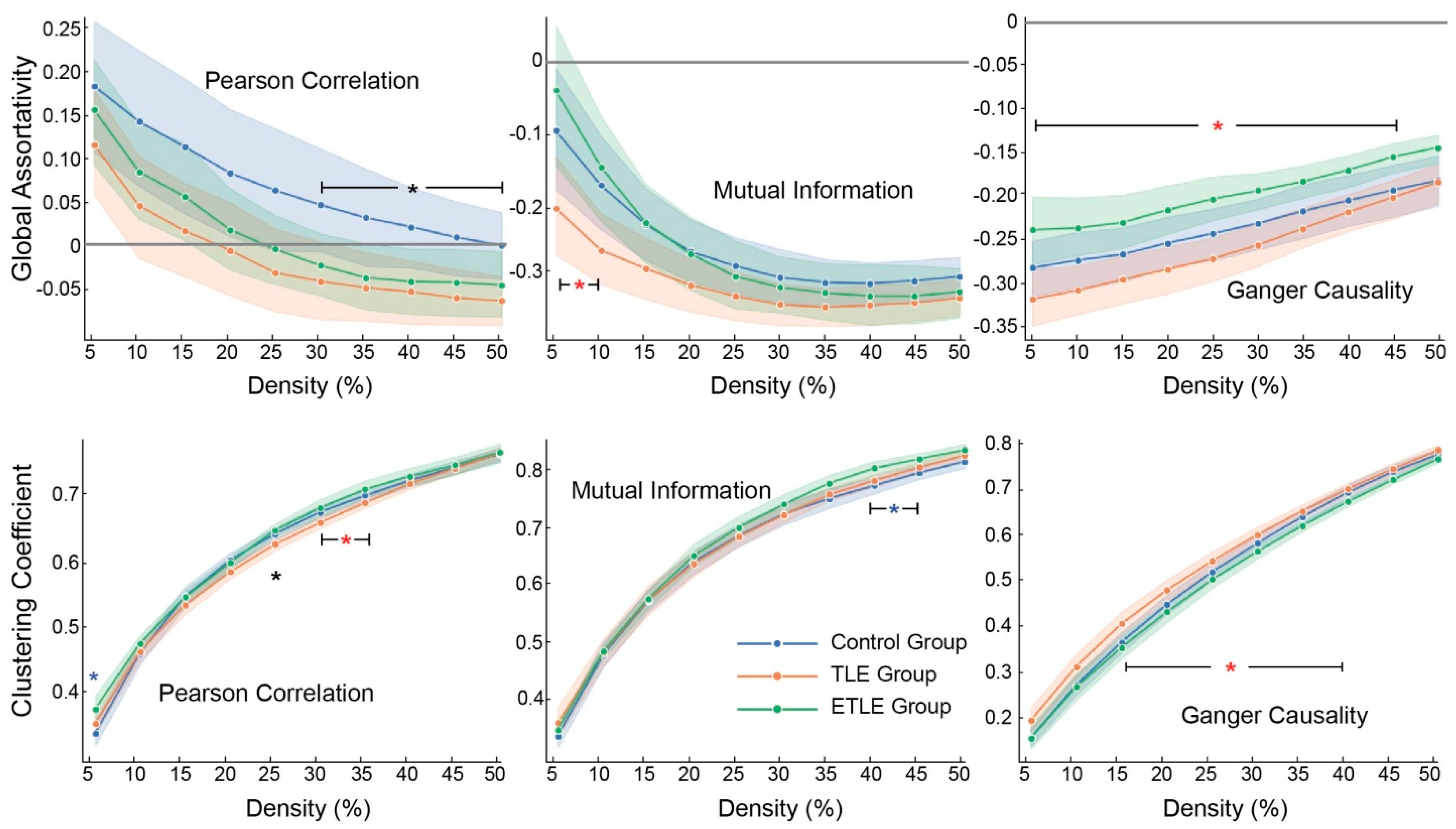
3.1. Topological Characteristics

The comparison between the global topological features, including global assortativity, efficiency, the mean clustering coefficient, and the number of components, was implemented for the three types of graphs (Pearson, MI, Granger causality) for all density levels. The results of all the global topological features comparison are presented in

Table 5. Global topological features comparison.

Global Topological Features	HC vs. TLE	HC vs. ETLE	TLE vs. ETLE	Metric	Density Level
Global assortativity	↑			Pearson correlation	30–50%
			↓	Mutual information	5–10%
			↓	Granger causality	5–45%
Global efficiency	↑			Pearson correlation	45–50%
			↓	Pearson correlation	30–50%
			↑	Granger causality	5%
Global clustering coefficient		↓		Pearson correlation	5%
	↑			Pearson correlation	25%
			↓	Pearson correlation	30–35%
		↓		Mutual information	40–45%
			↑	Granger causality	15–40%
		↓		Pearson correlation	5%
	↑			Pearson correlation	25%
Number of components	↓			Pearson correlation	40–50%
			↑	Pearson correlation	30–50%
		↑		Granger causality	5%

Note: The upwards/downwards arrow (↑/↓) indicates that the group has statistically significant higher/lower values, respectively. When there is no arrow, there is no statistically significant result. The metric of the test is shown in the fourth column. The fifth column presents the graph’s density level when there was a statistically significant result. The dash denotes that the difference was observed in all the density levels from the starting percentage to the final with a step of 5%.

.

From the topological characteristics analysis, the features that displayed significant differences among the three groups in all the connectivity methodologies were the global assortativity and the mean clustering coefficient (Figure 2). Specifically, in the Pearson correlation analysis, the healthy control displayed positive values of assortativity in all density levels. On the contrary, TLE patients exhibited disassortative functional networks for density levels higher than 30%. In higher density levels (above 45%), the TLE group showed lower values of global efficiency when compared to the other two groups. Interestingly, ETLE patients presented an increased mean clustering coefficient compared to the other two groups. Further, when the density level is more than 40%, TLE patients presented more components compared to the other two groups.

The graphs that evaluate the functional connectivity with the non-linear metric of MI present comparable topological features between the control and the TLE group. When 5% or 10% of the highest total edges are preserved, ETLE patients have higher assortativity compared to the TLE group. All the groups have disassortative graphs in all the density levels. In higher levels of density (40–45%) of the MI graphs, ETLE patients presented higher levels of clustering coefficient on average, compared to the graphs of the control group.

Concerning the Granger causality network, controls present similar topological features with each of the two patient groups, with significant differences being observed between TLE and ETLE groups. Specifically, TLE patients present graphs with higher clustering coefficient, and lower values of assortativity compared to ETLE group in most density levels. When we keep only the highest 5% of the connectivity values in the graph, the TLE patients show a more integrated graph compared to the ETLE patients (higher global efficiency), and the number of components is significantly lower in the ETLE group compared to controls.

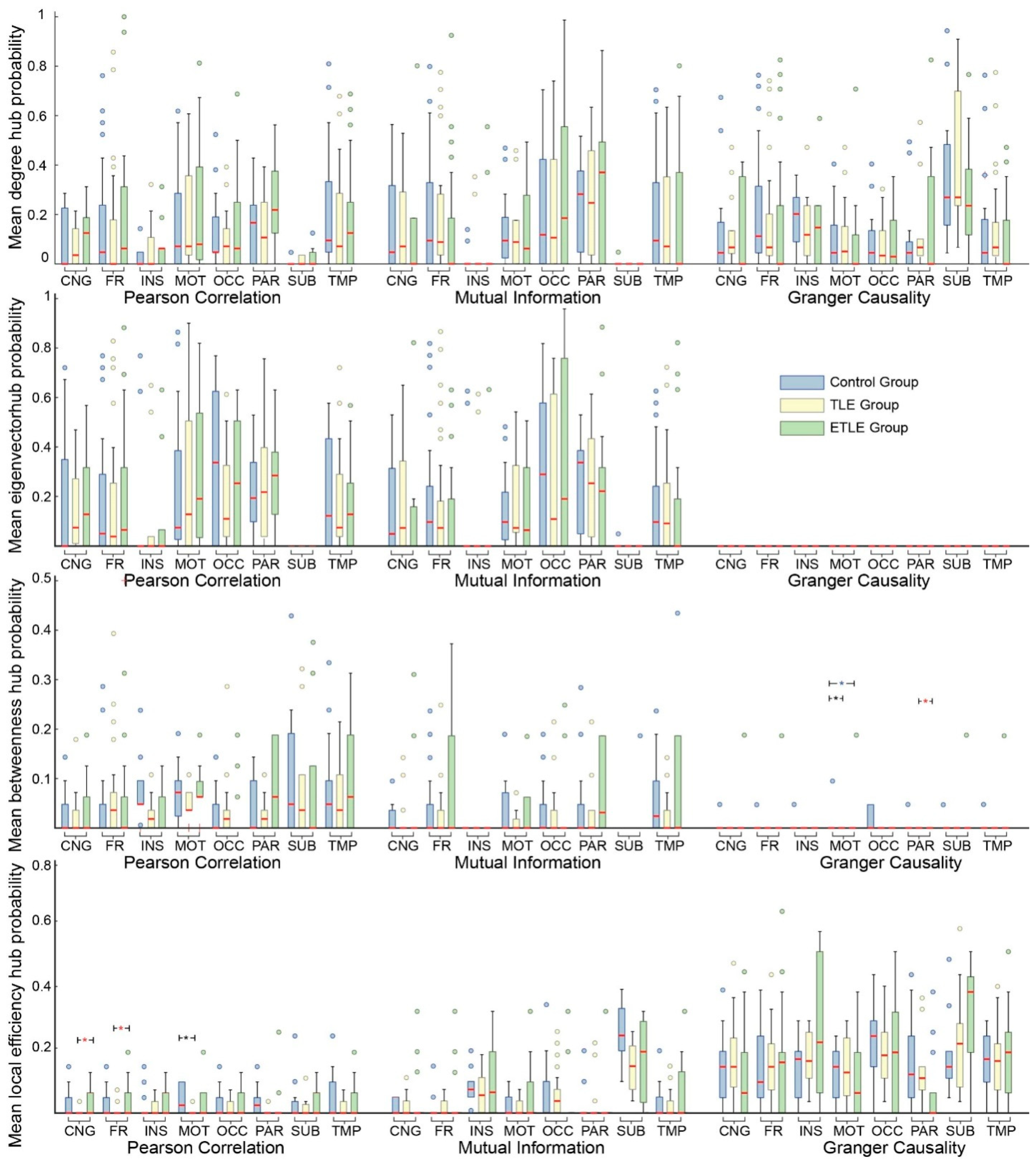
3.2. Hub Probabilities in Regions of Interest

The threshold on the hub probability of the ROIs is defined within each of the three groups and it is different for the three types of connectivity metrics, resulting in 9 different thresholds. In the Pearson correlation graph network analysis, the thresholds that were used to identify the hubs of each group were: p_R,ETLE > 0.55, p_R,TLE> 0.48, and p_R,C> 0.56. According to those thresholds, the hub regions presented in all groups in both hemispheres were as follows: the superior frontal gyrus (SFG), the superior parietal gyrus (SPG), the postcentral (PostCG) and precentral gyrus (PreCG), the precuneus (PCUN), the middle temporal gyrus (MTG), and the lateral aspect of the superior temporal gyrus (STGlat). In the left hemisphere, all groups have a hub with the supramarginal gyrus (SMG), and in the right hemisphere, the middle occipital gyrus (MOG) and the superior temporal sulcus (STS) (Figure 3). The highest probabilities in all groups are reported in Appendix C.

We observed a hub reorganization between the control group and the patients, explained through the differences in hub probabilities. The probability distribution indicated that the superior occipital gyrus (SOG) was identified in the control group with a hub probability of more than 61% in both hemispheres (61.9% the left SOG, 71.4% the right SOG), while the same probability was less than 36% for the TLE group (35.7% the left SOG, 32.1% the right SOG) and less than 50% for the ETLE group (37.5% the left SOG, 50% the right SOG). Furthermore, the bilateral Cuneus (CUN) demonstrated decreased probability in both patient groups compared to controls. Specifically, the left CUN hub probability was 66.7% in controls, 46.4% in TLE patients, and 31% in ETLE patients, while the right CUN hub probability was 71% for the controls, 42.9% in the TLE, and 50% in the ETLE groups. Another deviation that was observed in the patients’ hubs was in the left inferior occipital gyrus (IOG), where the control group showed a hub probability of 76.2% while the patient groups were significantly lower (39% for the TLE patients, 43.8% for the ETLE patients). Finally, the paracentral gyrus (ParaCG) was deemed as a region with a key role in the ETLE graphs, with 68.75% hub probability bilateral, while the bilateral hub probability for the control group was 38% and for the TLE was lower than 50% (46.43% in the left hemisphere and 42.86% in the right).

Regarding the MI graph networks, most of the hub regions did not display significant differences among the three groups (Figure 4). In the MI graph analysis, the thresholds that corresponded to the hub probabilities for each of the three groups were: p_R,ETLE > 0.56, p_R,TLE > 0.48, and p_R,C > 0.49. The highest probabilities in all groups are reported in Appendix C. The brain regions found as hubs in both hemispheres in all groups were more posterior regions, mainly in the occipital lobe as well as the superior parietal gyrus and the posterior central gyrus. The hubs presented unilaterally in all groups were the left CUN and the right ParaCG. Interestingly, the right CUN was presented in most patients’ MI graphs with higher hub probability values compared to the control group (hub probability was 60.7% in the TLE and 81% in the ETLE group, but only 47.6% in the controls). Similarly, the right angular gyrus (ANG) was identified as an important brain region in all ETLE patients and in 64.3% of TLE patients but displayed lower hub probability (47.6%) in the controls. On the contrary, the regions of left PCUN, left subparietal sulcus (subparS) and right posterior-ventral part of the cingulate gyrus (vPCC) demonstrated over 50% hub probability in the control group but less than 20% hub probability in the ETLE group. Those regions are not identified as hubs in the TLE group either, since they present hub probabilities lower than 48% (46.43% for the left PCUN and the right vPCC, 32.15% for the left subparS).

Concerning the Granger causality graph analysis, we employed three of the four centrality measures since eigenvector centrality can only be applied to undirected graphs. The thresholds applied to reveal the hubs in the directed graphs for the three groups were: p_R,ETLE > 0.57, p_R,TLE > 0.53, and p_R,C > 0.52. Notably, the hubs identified from the Granger causality directional graphs differ significantly from those reported in the Pearson correlation and MI graphs (Figure 5). In detail, the hub ROIs observed in both hemispheres in all groups include the subcallosal gyrus, the anterior transverse collateral sulcus of the occipital lobe, the medial olfactory orbital sulcus, and the pallidum. Additionally, hub nodes common to all groups in the right hemisphere include the gyrus rectus of the frontal lobe, the right amygdala, and the right thalamus. Notably, the regions with the highest probabilities in all groups are the right olfactory sulcus of the frontal lobe and the right pallidum, with the latter consistently identified as a hub ROI in all individuals of the TLE and ELTE groups, and in 90.48% of the controls. However, there are regions presented as hubs only in the control group, such as the left parahippocampal gyrus (Parahip G) and the left planum polare of the superior temporal gyrus (STG polar). ETLE patients present low hub probability (31.25%) in the left parahippocampal gyrus, while it is identified as a hub for 50% of the TLE patients and 57.14% of the controls. The pole of STG presents 61.9% hub probability in the control group but less than 50% hub probability in both patient groups (46.4% in the TLE group, 43.75% in the ETLE group). On the other hand, the right parahippocampal gyrus presents high hub probabilities in the patients (64.3% in TLE group, 68.75% in ETLE group), but it is not a hub for the controls (38.1% hub probability). In the subcortical areas, the right putamen and the left thalamus are identified as hubs in the TLE and ETLE groups with hub probabilities higher than 60%, but not in the controls where the hub probability is 47.6%.

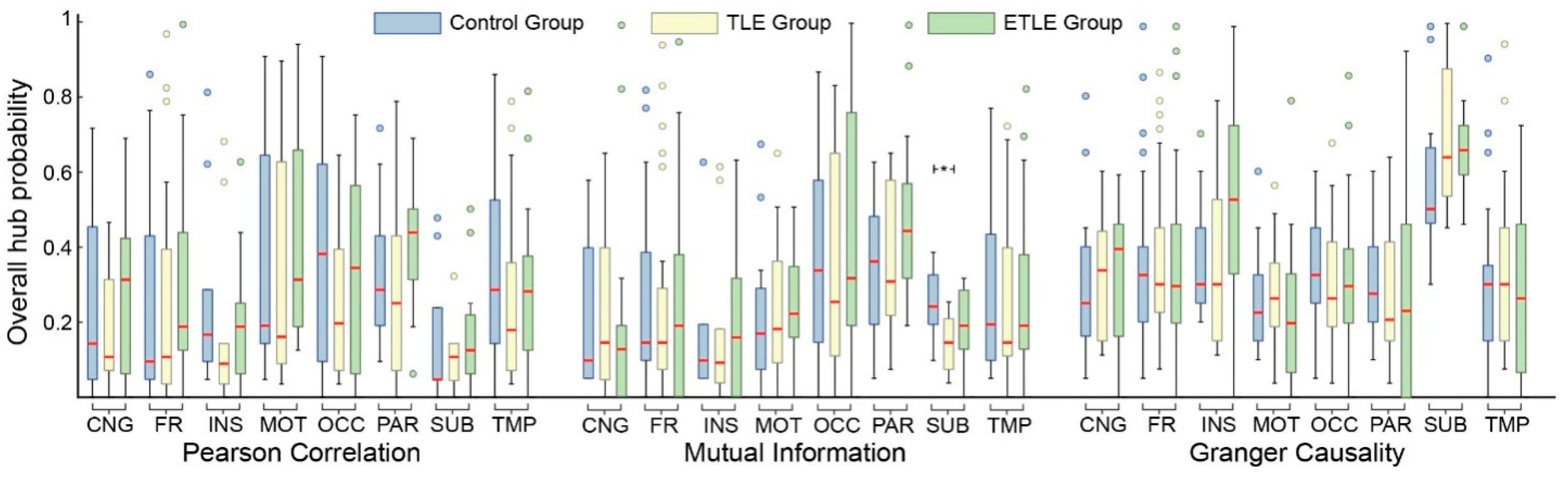
3.3. Hub Probabilities in Brain Sectors

We employed a statistical evaluation of anatomical subdivisions within the brain (brain sectors), each incorporating several ROIs (extended results can be found in Supplementary Materials). This procedure was applied separately for each centrality measure and each graph, while additionally implemented for the overall hub probability, defined as the mean hub probability of the ROIs included in each brain sector, regardless of the centrality measure. Figure 6 presents the mean centrality-specific hub probabilities within the eight brain sectors, for each of the three groups (C, TLE, ETLE). Similarly, Figure 7 displays the overall mean hub probability within the brain sectors.

In the Pearson graphs, the hubs based on the degree centrality hub probability are mainly located in the motor area for both patient groups. On the other hand, the control group presents most of the degree centrality hubs in the temporal lobe. The highest betweenness centrality hub probability is observed in the subcortical areas in all three groups. In the local efficiency hub probability, significant differences were indicated between ETLE and TLE patients in the frontal lobe and the cingulate cortex. Similarly, the control group displayed statistically significantly higher values compared to the TLE group in the motor areas. In the MI graphs, the three groups displayed similar hub probabilities, regardless of the centrality measure. Most of the hubs based on the degree centrality hub probability were observed in the parietal lobe. Interestingly, although all centrality measures indicated very low values and therefore close to zero hubs in the subcortical area, the local efficiency hub probability had its highest values there.

In the Granger causality graphs, the subcortical regions presented higher values in the degree centrality hub probability. This was also observed in the local efficiency hub probability values. The betweenness centrality hub probability displayed extremely low (close to zero) hub probability values. Despite this, there were a few hubs presented in the motor and parietal areas that were able to influence the mean values and thus display significant differences among the groups.

Of note is that the eigenvector centrality hub probability had comparable results with the degree centrality in both Pearson correlation and MI. As we mentioned in the methodology section, the eigenvector centrality can be calculated only for nodes of undirected graphs and hence, it is not defined for the graphs of Granger causality.

In the overall hub probability, the highest values in the Pearson correlation graphs were indicated in the motor area and the parietal lobe for TLE and ETLE patients, while in the control group, the occipital lobe presented the highest values, compared to the other brain sectors. The occipital lobe predominance was also observed in the MI graphs, although a significantly higher overall hub probability was found in the subcortical regions of the control group compared to the TLE patients. Meanwhile, Granger causality indicated the highest hub overall probability values for all groups in the subcortical regions.

4. Discussion

This study introduces a methodological approach to overcome existing limitations in the analysis of hub regions in epilepsy research. Unlike traditional approaches that solely rely on degree centrality, we employ four different centrality measures to evaluate the importance of regions of interest (ROIs) in connectivity networks. This inclusion allows the emergence of hubs based not only on the number of their connections but on a variety of nodal features that reveal their significance in the graph, such as their ability to bridge regions through a short path length. Additionally, instead of averaging connectivity values across groups, we analyze hubs at the individual level to maintain each subject’s connectivity patterns and minimize averaging bias. The proposed scheme offers promising findings that could potentially pave the way for future research in epilepsy biomarker discovery.

4.1. Brain Reorganization

In the comparison of global topological features, the healthy control group presents statistical differences with the TLE group only in the Pearson correlation graphs. Our analysis revealed lower values of global assortativity, global efficiency, and mean clustering coefficient values in TLE patients compared to healthy controls, particularly at density levels exceeding 25%. Although the reduction of global efficiency observed in TLE patients is supported by similar studies [23,24,25,26,27,28], it is worth mentioning that other researchers report contradictory findings [31,53]. In a similar manner, TLE patients display lower mean clustering coefficient values, with some studies reporting comparable results [24,26,27,28,31,53], while others suggest a higher global clustering coefficient for patients with focal epilepsy compared to controls [25].

This could be related to the fact that there are methodological differences between those studies, such as the definition of the ROIs with different atlases, and the threshold methods applied [54]. For instance, Mazrooyisebdani et al. [31] applied automated anatomical labeling (AAL) and temporal correlations and asserted that individuals with temporal lobe epilepsy (TLE) exhibit functional networks characterized by higher global efficiency and lower clustering coefficient compared to healthy controls. However, most of the studies report similar results to our analysis, where TLE patients present lower global integration (reduced efficiency) and segregation (reduced mean clustering coefficient) in their graphs compared to the controls. Interestingly, those topological features have been related to cognitive deficits observed in chronic epilepsy [28]. The ETLE group presents increased mean clustering coefficient compared to the control group in the undirected graphs of Pearson correlation and MI, at different density levels (40–45% in the MI and 5% in the Pearson correlation graph). Previous studies report similar changes in children with frontal lobe epilepsy, where patients presented efficient communication within specific clusters of ROIs but limited connection between the clusters [55]. Since half of our cohort in the ETLE group are patients with frontal lobe epilepsy, no generalization can be made in all extratemporal lobe epilepsies, but further investigation should be performed with bigger cohorts. We find no difference in the global efficiency of the ETLE groups compared to controls. In line with our results, Pedersen et al. [56] employed a brain mask consisting of 278 nodes and a Pearson correlation method, reporting no difference in the path length but increased segregation in patients with ETLE compared to controls. We find statistical differences in the brain topological features of the TLE and ETLE group that may include useful information regarding the organization of the epileptic network in the two types of epilepsy. TLE patients exhibit more disassortative graphs compared to ETLE in lower density levels of the MI graphs (5–10%) and in almost all the density levels of the Granger causality graphs. Further, the TLE group exhibits a greater number of components in relation to the other two groups at density levels exceeding 40%. This could be due to network edges present in the TLE graphs with weak connectivity strength although acting as bridges. In the undirected graphs of Pearson correlation, at 30–35% density level, ETLE graphs show topological characteristics more aligned with small-world architecture (higher clustering coefficients and global efficiency) in comparison to the TLE group. As such, ETLE patients can form clusters of regions and ensure communication between distant parts of the brain by short path lengths concurrently. On the opposite, the directed graphs of Granger causality indicate that ETLE patients present lower mean clustering coefficient in most of the density levels (from 15% to 40%) and lower global efficiency at the lowest density level (5%) compared to TLE group. The meta-analysis of Diessen et al. [25] suggests that patients with focal epilepsy have increased clustering coefficient and decreased efficiency compared to controls, tending towards a regular network topology, but contrary to our results, they find no difference between the subgroups of TLE and ETLE patients. In-vivo studies reveal that the segregated topology observed in drug-resistant TLE patients, with increased local connectivity and disrupted long-distance connectivity could serve as a mechanism that regulates seizure propagation [57]. Our study suggests that the mean clustering coefficient is a measure presenting differences between the two epilepsy groups (temporal and extratemporal), but the outcome is conflicting between the directed and undirected graphs. This observation is in line with the study of Prando et al. [58] where they compare the topological features between the effective connectivity graphs (directed connectivity), estimated using dynamic causal modeling and the functional connectivity graphs (undirected connectivity) of healthy subjects, and report differences between the two connectivity methods especially in the nodal clustering coefficient. In the future, more studies should investigate the impact of directionality in functional connectivity networks, and on the tendency of brain regions to form clusters.

Although overall differences among the various techniques are to be expected due to the dissimilar algorithmic designs, it should be noted that the patients displayed a disassortative graph in thresholds higher than 25% in all cases. In addition to this, TLE patients have more disassortative graphs compared to the other groups, with significant differences reported in all connectivity methods. Since disassortative graphs are more vulnerable to targeted attacks [59], the removal or the dysfunction of some brain regions would create more isolated regions in the TLE group compared to the ETLE group, with consequences on the size of the largest connected component of the graph. However, it is not clear if this disruption in connectivity, expressed by the vulnerability of the graph, would be beneficial for the epilepsy group [60]. As such, the vulnerability may assist in the control of the seizure propagation reducing the possible pathways of the epileptic discharge but could also imply the dysfunction of brain regions and disorganization of functional networks (such as the default mode network), with an impact on the pathophysiology of patients. The importance of global assortativity as a clinical biomarker for epilepsy has been highlighted in previous studies, reporting that patients with drug-resistance focal epilepsy had more disassortative graphs compared to patients who had positive responses in anti-epileptic drugs [61]. In our study, all the patients (TLE and ETLE) present drug resistance, but only TLE patients present lower assortativity compared to controls.

4.2. Key Region Mapping

Regarding specific brain areas from the analysis of the hub regions SFG, SPG, PCUN, MOG, SOG, ParaCG, Calcarine, and ITG were identified in Pearson correlation and MI graphs. The significance of these regions is corroborated by various studies [62,63,64,65]. The review of Heuvel and Sporns designates the PCUN, SFG, and SPG regions as both structural and functional hubs [64]. In line with this review, Lin et al. [65] suggested that bilateral PCUN, SFG and SPG are part of a set of regions that are strongly connected to each other and they observed that TLE patients show decreased functional connectivity especially between ROIs that belong to rich-club. On the other hand, bilateral CUN presented low probability values of being a hub in TLE and ETLE patients, while it is identified as a hub in most control subjects. This is supported by other studies indicating that surgery in children with epilepsy improved significantly the nodal efficiency of cuneus [23,66]. Also, the study of Galovic et al. [67] reports a progressive cortical thinning in the left CUN, observed in patients with left temporal lobe and right frontal lobe epilepsies.Furthermore, in the Pearson graphs an alteration in the hubs of the occipital lobe was observed in the bilateral SOG and IOG, demonstrating low hub probability in both TLE and ETLE groups while in healthy controls this probability was high. Previous studies have also found decreased regional homogeneity in TLE patients compared to controls in these regions (SOG, IOG, and CUN), suggesting that abnormalities in brain regions which act as central nodes could deter efficient communication and integration of information across different parts of the brain [68]. On the contrary, in the MI graphs, ANG was identified as a hub region for all ETLE patients and 64% of the TLE patients but displayed less than 50% probability of being a hub region in the control group. Similar to this outcome, previous studies report increased nodal parameters, such as betweenness and degree centrality, in the ANG of patients with temporal lobe and juvenile myoclonic epilepsies compared to controls [69,70]. Since the angular gyrus is part of the inferior parietal cluster of the default mode network (DMN), the increased connectivity of this region may lead to the spread of the seizure within the DMN and can be the reason for cognitive difficulties observed in patients with TLE [71,72,73].

Regarding the causal relationship between ROIs, the Granger causality graphs in the control group identified the left parahippocampal gyrus and the left STG polar as hubs. However, those regions show lower hub probability in both TLE and ETLE epilepsy groups. In the study by Galovic et al. [67] the left STG presents progressive atrophy in patients with left TLE and they provide evidence of increased progressive atrophy of the parahippocampal gyrus in the TLE compared to patients with frontal lobe epilepsy. In our study, the significance of parahippocampal gyrus is also highlighted in the patient groups but only in the right hemisphere. Since the majority of the patients have left hemisphere lateralized epilepsy (68.2% of total patients), this could imply a disturbance of this region ipsilateral to the seizure onset. Moreover, in the directed Granger causality graphs, the subcortical regions were significant across all groups, while the amygdala and the pallidum were the most prominent. This is corroborated by recent studies indicating the subcortical areas of pallidum, putamen, and thalamus as brain connector hubs, suggesting their multiple roles in the efficient information flow of the healthy brain [63,74]. The subcortical regions play a key role in seizure propagation, especially the thalamus [75,76]. There is evidence supporting that reduction in the grey matter of thalamus and hippocampus may be related to the severity of epilepsy [77]. A study that investigated the presurgical resting-state fMRI networks of TLE patients proposed the nodal topological features of thalamus as biomarkers for the prediction of surgery outcomes, as patients who did not achieve seizure freedom after surgery presented higher nodal degree and eigenvector centrality values in the thalamus compared to patients who achieved seizure freedom [78]. The study of Park et al. [79] underlines the significance of this area as a possible biomarker for focal epilepsy since it presents increased nodal topological features in patients compared to the healthy controls. Further, they suggest that the increased connectivity of the pallidum can be responsible for the generation of epileptic seizures. Contrary to this assumption, the pallido-cortical pathway has been assumed to be the mechanism that regulates the absence seizures [80]. In our study, we found that Granger causality can depict the importance of subcortical areas both in patients and controls, with most prominent regions the right amygdala and thalamus, as well as the bilateral pallidum. Those regions are identified as hubs in most of the subjects due to their high values of degree centrality and hence, they regulate the communication within the graph through out-flow and in-flow connections

4.3. Network Analysis Comparisons

Further investigation regarding the eight brain sectors revealed that hub regions are dependent on the type of graph. For instance, the subcortical regions had almost zero mean degree hub probability in the undirected graphs of Pearson and MI, while in the directed graph of Granger causality, their role was crucial across all three groups. The causal influence exerted from deep brain structures to the cortical areas has been highlighted in various studies [81,82]. Although, this causality has not been found before in graph characteristics, or it was not as prominent as in our study. On the other hand, the subcortical regions presented non-zero probability values both in the mean betweenness hub probability of the Pearson connectivity graphs and in the mean local efficiency hub probability of the MI graphs, in all groups. In the directed graphs of Granger causality, all the groups present high hub probability levels in the subcortical area, based on the degree centrality and the local efficiency. This suggests that the subcortical regions are significant in every type of graph, but their role differs based on the metric. In the Pearson graph, the subcortical regions may display a higher role as network mediators, minimizing the distances in the interaction between other regions. The review of Herbet and Duffau proposes the meta-networks of the brain, based both on anatomic and functional connectivity, and suggested the mediating role of subcortical regions (especially thalamus, amygdala, and hippocampus) in pathways supporting higher cognitive functions [83].

In the MI and Granger graphs, the mean local efficiency hub probability denotes that the removal of those nodes would affect the efficient information flow in the whole brain network. Further, in the Granger graphs, this brain sector includes most of the hubs based on the degree centrality, suggesting that the regions with most connections (inflow and outflow) are included in the deep brain structures. On this premise, the study of van den Heuvel and Sporns [84] analyzed the anatomical connectivity of the brain, showing that the subcortical regions of the thalamus, putamen, and hippocampus are recognized as hubs using all types of centralities mentioned in our study. They concluded by classifying those regions as ‘provincial hubs,’ meaning that their value is profound mainly at a local level. In our study, we confirm this regional importance of the subcortical regions, both in the MI and Granger causality graphs, where the values of the mean local efficiency hub probability are high compared to the other brain sectors.

Concerning the mean local efficiency hub probability of the Brain Sectors in the Pearson graphs, the TLE patients show near-zero values, with statistical differences compared to the ETLE group in the cingulate cortex and the frontal lobe, as well as in the motor area compared to the controls. This outcome, combined with the fact that we found the lowest global efficiency in the TLE group compared to the other two groups, suggests that the brain regions of TLE patients do not communicate locally in such an efficient way, and this nodal observation also affects the overall efficiency in the communication of the brain network. The study of Liu et al. [85] verifies this, suggesting that TLE patients present lower nodal efficiency in many regions, resulting in significant reduction of global efficiency metrics compared to healthy controls. On the other hand, the mean local efficiency hub probability of the ETLE patients presents similar values with the control group. The divergence observed between the two types of epilepsy may include information regarding the complexity of the epileptic network, where the different patterns of hub reorganization might correspond to the attempt of the epileptic brain to mitigate neurocognitive deficits. Although many studies underlie the altered hub distribution as a biomarker of epilepsy, there is limited knowledge regarding the connection of this mechanism to the clinical features of the disease [32].

Regarding the overall hub probability, the insula and the subcortical regions presented conflicting results, being the ones with the higher values in the Granger causality and the lowest in the undirected graphs. We can hence conclude that the ROIs included in the insula and the subcortical structures have a causal influence on (or from) other regions of the graph. In a similar manner, the parietal lobe displayed higher values in the Pearson and MI graphs and the lowest overall hub probability in the Granger causality. This further supports the premise that the topology of the brain graph can vary depending on whether the graph is based on functional or effective connectivity measures [86]. This variability underscores the need for using multiple connectivity measures to obtain a comprehensive understanding of brain network dynamics and hub regions in patients

4.4. Limitations and Future Work

When interpreting the results of this study, certain limitations need to be acknowledged. Initially, it is important to note that the size of the cohort, particularly in the ETLE group (16 patients), reduces the statistical power of our results. Further studies with larger cohorts would narrow the confidence intervals in the evaluation of hub probabilities. Secondly, our study does not differentiate between left and right TLE and ETLE patients. This decision was made because of the small sample size and after ensuring there is no statistical significance in the metrics within the TLE and ETLE groups with left/right seizure onset hemispheres. However, graph-theory metrics may vary, and future investigation is encouraged to explore whether hub localization depends on the hemisphere of the epilepsy onset. Lastly, our evaluation focuses solely on static connectivity using linear and non-linear metrics to quantify correlation and causality between ROIs. Future research incorporating dynamic analysis of hubs could enhance our understanding of the stability of nodes, which play crucial roles in information flow within different types of graphs.

5. Conclusions

This study investigates the brain network topological variations between patients with TLE and ETLE using both directed and undirected network connectivity methods alongside various graph-theory metrics. Given that different graph-theory frameworks and estimation measures can lead to significant variability among study results, we address these constraints by evaluating the importance of regions of interest (ROIs) using four centrality measures across three different connectivity techniques (Pearson correlation, Mutual Information, and Granger causality). Instead of averaging brain network data, we analyze the hubs of each subject individually and then create a hub probability based on their presence within each group, thereby minimizing averaging bias. Our findings reveal distinct topological differences between the two epilepsy groups, with TLE patients displaying more disassortative graphs at lower density levels compared to ETLE patients. We also uncover variations in hub regions across different network metrics, highlighting the need to consider various centrality measures for a comprehensive understanding of brain network dynamics in epilepsy. Furthermore, we explore the global centralization features and hub probabilities of each ROI across all subjects and groups at different density thresholds, revealing regional alterations that underscore the unique characteristics of each epilepsy type. This comprehensive approach offers insights into potential biomarkers for type-specific epilepsy diagnosis and treatment, emphasizing the importance of hub reorganization as a possible predictor of network restructuring in epilepsy.

References

1. Epilepsy. Available online: https://www.who.int/news-room/fact-sheets/detail/epilepsy (accessed on 26 July 2024).
2. Fisher, R.S.; Acevedo, C.; Arzimanoglou, A.; Bogacz, A.; Cross, J.H.; Elger, C.E.; Engel Jr, J.; Forsgren, L.; French, J.A.; Glynn, M.; et al. ILAE Official Report: A Practical Clinical Definition of Epilepsy. Epilepsia 2014, 55, 475–482. [Google Scholar] [CrossRef] [PubMed]
3. Brodie, M.J.; Barry, S.J.E.; Bamagous, G.A.; Norrie, J.D.; Kwan, P. Patterns of Treatment Response in Newly Diagnosed Epilepsy. Neurology 2012, 78, 1548–1554. [Google Scholar] [CrossRef] [PubMed]
4. Strzelczyk, A.; Aledo-Serrano, A.; Coppola, A.; Didelot, A.; Bates, E.; Sainz-Fuertes, R.; Lawthom, C. The Impact of Epilepsy on Quality of Life: Findings from a European Survey. Epilepsy Behav. 2023, 142, 109179. [Google Scholar] [CrossRef] [PubMed]
5. Tani, A.; Adali, N. Cognitive Disorders, Depression and Anxiety in Temporal Lobe Epilepsy: An Overview. J. Biosci. Med. 2024, 12, 77–93. [Google Scholar] [CrossRef]
6. Jain, P.; Smith, M.L.; Speechley, K.; Ferro, M.; Connolly, M.; Ramachandrannair, R.; Almubarak, S.; Andrade, A.; Widjaja, E.; Team, P.S. Seizure Freedom Improves Health-Related Quality of Life after Epilepsy Surgery in Children. Dev. Med. Child Neurol. 2020, 62, 600–608. [Google Scholar] [CrossRef]
7. Swarup, O.; Waxmann, A.; Chu, J.; Vogrin, S.; Lai, A.; Laing, J.; Barker, J.; Seiderer, L.; Ignatiadis, S.; Plummer, C.; et al. Long-Term Mood, Quality of Life, and Seizure Freedom in Intracranial EEG Epilepsy Surgery. Epilepsy Behav. 2021, 123, 108241. [Google Scholar] [CrossRef]
8. Lehnertz, K.; Bröhl, T.; Wrede, R. von Epileptic-Network-Based Prediction and Control of Seizures in Humans. Neurobiol. Dis. 2023, 181, 106098. [Google Scholar] [CrossRef]
9. Gleichgerrcht, E.; Keller, S.S.; Drane, D.L.; Munsell, B.C.; Davis, K.A.; Kaestner, E.; Weber, B.; Krantz, S.; Vandergrift, W.A.; Edwards, J.C.; et al. Temporal Lobe Epilepsy Surgical Outcomes Can Be Inferred Based on Structural Connectome Hubs: A Machine Learning Study. Ann. Neurol. 2020, 88, 970–983. [Google Scholar] [CrossRef]
10. De Palma, L.; Benedictis, A.D.; Specchio, N.; Marras, C.E. Epileptogenic Network Formation. Neurosurg. Clin. 2020, 31, 335–344. [Google Scholar] [CrossRef]
11. Cohen, M.S.; Bookheimer, S.Y. Localization of Brain Function Using Magnetic Resonance Imaging. Trends Neurosci. 1994, 17, 268–277. [Google Scholar] [CrossRef]
12. Feng, X.; Piper, R.J.; Prentice, F.; Clayden, J.D.; Baldeweg, T. Functional Brain Connectivity in Children with Focal Epilepsy: A Systematic Review of Functional MRI Studies. Seizure Eur. J. Epilepsy 2024, 117, 164–173. [Google Scholar] [CrossRef] [PubMed]
13. Park, H.-J.; Friston, K. Structural and Functional Brain Networks: From Connections to Cognition. Science 2013, 342, 1238411. [Google Scholar] [CrossRef] [PubMed]
14. Friston, K.J.; Frith, C.D.; Liddle, P.F.; Frackowiak, R.S.J. Functional Connectivity: The Principal-Component Analysis of Large (PET) Data Sets. J. Cereb. Blood Flow Metab. 1993, 13, 5–14. [Google Scholar] [CrossRef] [PubMed]
15. van den Heuvel, M.P.; Hulshoff Pol, H.E. Exploring the Brain Network: A Review on Resting-State fMRI Functional Connectivity. Eur. Neuropsychopharmacol. 2010, 20, 519–534. [Google Scholar] [CrossRef] [PubMed]
16. Spencer, S.S. Neural Networks in Human Epilepsy: Evidence of and Implications for Treatment. Epilepsia 2002, 43, 219–227. [Google Scholar] [CrossRef]
17. Boerwinkle, V.L.; Mirea, L.; Gaillard, W.D.; Sussman, B.L.; Larocque, D.; Bonnell, A.; Ronecker, J.S.; Troester, M.M.; Kerrigan, J.F.; Foldes, S.T.; et al. Resting-State Functional MRI Connectivity Impact on Epilepsy Surgery Plan and Surgical Candidacy: Prospective Clinical Work. J. Neurosurg. Pediatr. 2020, 25, 574–581. [Google Scholar] [CrossRef]
18. Foit, N.A.; Bernasconi, A.; Bernasconi, N. Functional Networks in Epilepsy Presurgical Evaluation. Neurosurg. Clin. 2020, 31, 395–405. [Google Scholar] [CrossRef]
19. Bernhardt, B.C.; Bonilha, L.; Gross, D.W. Network Analysis for a Network Disorder: The Emerging Role of Graph Theory in the Study of Epilepsy. Epilepsy Behav. 2015, 50, 162–170. [Google Scholar] [CrossRef]
20. Farahani, F.V.; Karwowski, W.; Lighthall, N.R. Application of Graph Theory for Identifying Connectivity Patterns in Human Brain Networks: A Systematic Review. Front. Neurosci. 2019, 13, 585. [Google Scholar] [CrossRef]
21. Larivière, S.; Bernasconi, A.; Bernasconi, N.; Bernhardt, B.C. Connectome Biomarkers of Drug-Resistant Epilepsy. Epilepsia 2021, 62, 6–24. [Google Scholar] [CrossRef]
22. Doucet, G.E.; Rider, R.; Taylor, N.; Skidmore, C.; Sharan, A.; Sperling, M.; Tracy, J.I. Presurgery Resting-State Local Graph-Theory Measures Predict Neurocognitive Outcomes after Brain Surgery in Temporal Lobe Epilepsy. Epilepsia 2015, 56, 517–526. [Google Scholar] [CrossRef] [PubMed]
23. Bernhardt, B.C.; Chen, Z.; He, Y.; Evans, A.C.; Bernasconi, N. Graph-Theoretical Analysis Reveals Disrupted Small-World Organization of Cortical Thickness Correlation Networks in Temporal Lobe Epilepsy. Cereb. Cortex 2011, 21, 2147–2157. [Google Scholar] [CrossRef] [PubMed]
24. Ai, H.; Yang, C.; Lu, M.; Ren, J.; Li, Z.; Zhang, Y. Abnormal White Matter Structural Network Topological Property in Patients with Temporal Lobe Epilepsy. CNS Neurosci. Ther. 2024, 30, e14414. [Google Scholar] [CrossRef] [PubMed]
25. Van Diessen, E.; Zweiphenning, W.J.E.M.; Jansen, F.E.; Stam, C.J.; Braun, K.P.J.; Otte, W.M. Brain Network Organization in Focal Epilepsy: A Systematic Review and Meta-Analysis. PLoS ONE 2014, 9, e114606. [Google Scholar] [CrossRef]
26. Ma, K.; Zhang, X.; Song, C.; Han, S.; Li, W.; Wang, K.; Mao, X.; Zhang, Y.; Cheng, J. Altered Topological Properties and Their Relationship to Cognitive Functions in Unilateral Temporal Lobe Epilepsy. Epilepsy Behav. 2023, 144, 109247. [Google Scholar] [CrossRef]
27. Haneef, Z.; Chiang, S. Clinical Correlates of Graph Theory Findings in Temporal Lobe Epilepsy. Seizure 2014, 23, 809–818. [Google Scholar] [CrossRef]
28. Vlooswijk, M.C.G.; Vaessen, M.J.; Jansen, J.F.A.; de Krom, M.C.F.T.M.; Majoie, H.J.M.; Hofman, P.A.M.; Aldenkamp, A.P.; Backes, W.H. Loss of Network Efficiency Associated with Cognitive Decline in Chronic Epilepsy. Neurology 2011, 77, 938–944. [Google Scholar] [CrossRef]
29. Stam, C.J. Hub Overload and Failure as a Final Common Pathway in Neurological Brain Network Disorders. Netw. Neurosci. 2024, 8, 1–23. [Google Scholar] [CrossRef]
30. Crossley, N.A.; Mechelli, A.; Scott, J.; Carletti, F.; Fox, P.T.; McGuire, P.; Bullmore, E.T. The Hubs of the Human Connectome Are Generally Implicated in the Anatomy of Brain Disorders. Brain 2014, 137, 2382–2395. [Google Scholar] [CrossRef]
31. Mazrooyisebdani, M.; Nair, V.A.; Garcia-Ramos, C.; Mohanty, R.; Meyerand, E.; Hermann, B.; Prabhakaran, V.; Ahmed, R. Graph Theory Analysis of Functional Connectivity Combined with Machine Learning Approaches Demonstrates Widespread Network Differences and Predicts Clinical Variables in Temporal Lobe Epilepsy. Brain Connect. 2020, 10, 39–50. [Google Scholar] [CrossRef]
32. Royer, J.; Bernhardt, B.C.; Larivière, S.; Gleichgerrcht, E.; Vorderwülbecke, B.J.; Vulliémoz, S.; Bonilha, L. Epilepsy and Brain Network Hubs. Epilepsia 2022, 63, 537–550. [Google Scholar] [CrossRef] [PubMed]
33. Gkiatis, K.; Garganis, K.; Benjamin, C.F.; Karanasiou, I.; Kondylidis, N.; Harushukuri, J.; Matsopoulos, G.K. Standardization of Presurgical Language fMRI in Greek Population: Mapping of Six Critical Regions. Brain Behav. 2022, 12, e2609. [Google Scholar] [CrossRef] [PubMed]
34. Dachena, C.; Casu, S.; Fanti, A.; Lodi, M.B.; Mazzarella, G. Combined Use of MRI, fMRIand Cognitive Data for Alzheimer’s Disease: Preliminary Results. Appl. Sci. 2019, 9, 3156. [Google Scholar] [CrossRef]
35. Jenkinson, M.; Beckmann, C.F.; Behrens, T.E.J.; Woolrich, M.W.; Smith, S.M. FSL. NeuroImage 2012, 62, 782–790. [Google Scholar] [CrossRef] [PubMed]
36. Greve, D.N.; Fischl, B. Accurate and Robust Brain Image Alignment Using Boundary-Based Registration. NeuroImage 2009, 48, 63–72. [Google Scholar] [CrossRef]
37. Jenkinson, M.; Bannister, P.; Brady, M.; Smith, S. Improved Optimization for the Robust and Accurate Linear Registration and Motion Correction of Brain Images. NeuroImage 2002, 17, 825–841. [Google Scholar] [CrossRef]
38. Beckmann, C.F.; Smith, S.M. Probabilistic Independent Component Analysis for Functional Magnetic Resonance Imaging. IEEE Trans. Med. Imaging 2004, 23, 137–152. [Google Scholar] [CrossRef]
39. Gkiatis, K.; Garganis, K.; Karanasiou, I.; Chatzisotiriou, A.; Zountsas, B.; Kondylidis, N.; Matsopoulos, G.K. Independent Component Analysis: A Reliable Alternative to General Linear Model for Task-Based fMRI. Front. Psychiatry 2023, 14, 1214067. [Google Scholar] [CrossRef]
40. Destrieux, C.; Fischl, B.; Dale, A.; Halgren, E. Automatic Parcellation of Human Cortical Gyri and Sulci Using Standard Anatomical Nomenclature. Neuroimage 2010, 53, 1–15. [Google Scholar] [CrossRef]
41. Fischl, B. FreeSurfer. Neuroimage 2012, 62, 774–781. [Google Scholar] [CrossRef]
42. Benesty, J.; Chen, J.; Huang, Y.; Cohen, I. Pearson Correlation Coefficient. In Noise Reduction in Speech Processing; Cohen, I., Huang, Y., Chen, J., Benesty, J., Eds.; Springer: Berlin/Heidelberg, Germany, 2009; pp. 1–4. ISBN 978-3-642-00296-0. [Google Scholar]
43. Kraskov, A.; Stögbauer, H.; Grassberger, P. Estimating Mutual Information. Phys. Rev. E 2004, 69, 066138. [Google Scholar] [CrossRef] [PubMed]
44. Granger, C.W.J. Investigating Causal Relations by Econometric Models and Cross-Spectral Methods. Econometrica 1969, 37, 424–438. [Google Scholar] [CrossRef]
45. Garrison, K.A.; Scheinost, D.; Finn, E.S.; Shen, X.; Constable, R.T. The (in)Stability of Functional Brain Network Measures across Thresholds. NeuroImage 2015, 118, 651–661. [Google Scholar] [CrossRef] [PubMed]
46. Newman, M.E.J. Assortative Mixing in Networks. Phys. Rev. Lett. 2002, 89, 208701. [Google Scholar] [CrossRef]
47. Latora, V.; Marchiori, M. Efficient Behavior of Small-World Networks. Phys. Rev. Lett. 2001, 87, 198701. [Google Scholar] [CrossRef]
48. Watts, D.J.; Strogatz, S.H. Collective Dynamics of ‘Small-World’ Networks. Nature 1998, 393, 440–442. [Google Scholar] [CrossRef]
49. Nesterov, A.I. On Clustering Coefficients in Complex Networks 2024. arXiv 2024, arXiv:2401.02999. [Google Scholar]
50. Freeman, L.C. A Set of Measures of Centrality Based on Betweenness. Sociometry 1977, 40, 35–41. [Google Scholar] [CrossRef]
51. Brandes, U. A Faster Algorithm for Betweenness Centrality. J. Math. Sociol. 2001, 25, 163–177. [Google Scholar] [CrossRef]
52. Newman, M.E.J. Finding Community Structure in Networks Using the Eigenvectors of Matrices. Phys. Rev. E 2006, 74, 036104. [Google Scholar] [CrossRef]
53. Liao, W.; Zhang, Z.; Pan, Z.; Mantini, D.; Ding, J.; Duan, X.; Luo, C.; Lu, G.; Chen, H. Altered Functional Connectivity and Small-World in Mesial Temporal Lobe Epilepsy. PLoS ONE 2010, 5, e8525. [Google Scholar] [CrossRef] [PubMed]
54. Stanley, M.L.; Moussa, M.N.; Paolini, B.; Lyday, R.G.; Burdette, J.H.; Laurienti, P.J. Defining Nodes in Complex Brain Networks. Front. Comput. Neurosci. 2013, 7, 169. [Google Scholar] [CrossRef] [PubMed]
55. Vaessen, M.J.; Braakman, H.M.H.; Heerink, J.S.; Jansen, J.F.A.; Debeij-van Hall, M.H.J.A.; Hofman, P.A.M.; Aldenkamp, A.P.; Backes, W.H. Abnormal Modular Organization of Functional Networks in Cognitively Impaired Children with Frontal Lobe Epilepsy. Cereb. Cortex 2013, 23, 1997–2006. [Google Scholar] [CrossRef] [PubMed]
56. Pedersen, M.; Omidvarnia, A.H.; Walz, J.M.; Jackson, G.D. Increased Segregation of Brain Networks in Focal Epilepsy: An fMRI Graph Theory Finding. NeuroImage Clin. 2015, 8, 536–542. [Google Scholar] [CrossRef]
57. Larivière, S.; Weng, Y.; Vos De Wael, R.; Royer, J.; Frauscher, B.; Wang, Z.; Bernasconi, A.; Bernasconi, N.; Schrader, D.V.; Zhang, Z.; et al. Functional Connectome Contractions in Temporal Lobe Epilepsy: Microstructural Underpinnings and Predictors of Surgical Outcome. Epilepsia 2020, 61, 1221–1233. [Google Scholar] [CrossRef]
58. Prando, G.; Zorzi, M.; Bertoldo, A.; Corbetta, M.; Zorzi, M.; Chiuso, A. Sparse DCM for Whole-Brain Effective Connectivity from Resting-State fMRI Data. NeuroImage 2020, 208, 116367. [Google Scholar] [CrossRef]
59. Al Musawi, A.F.; Roy, S.; Ghosh, P. Examining Indicators of Complex Network Vulnerability across Diverse Attack Scenarios. Sci. Rep. 2023, 13, 18208. [Google Scholar] [CrossRef]
60. Englot, D.J.; Konrad, P.E.; Morgan, V.L. Regional and Global Connectivity Disturbances in Focal Epilepsy, Related Neurocognitive Sequelae, and Potential Mechanistic Underpinnings. Epilepsia 2016, 57, 1546–1557. [Google Scholar] [CrossRef]
61. Park, K.M.; Cho, K.H.; Lee, H.-J.; Heo, K.; Lee, B.I.; Kim, S.E. Predicting the Antiepileptic Drug Response by Brain Connectivity in Newly Diagnosed Focal Epilepsy. J. Neurol. 2020, 267, 1179–1187. [Google Scholar] [CrossRef]
62. Yu, Y.; Qiu, M.; Zou, W.; Zhao, Y.; Tang, Y.; Tian, J.; Chen, X.; Qiu, W. Impaired Rich-Club Connectivity in Childhood Absence Epilepsy. Front. Neurol. 2023, 14, 1135305. [Google Scholar] [CrossRef]
63. Oldham, S.; Fornito, A. The Development of Brain Network Hubs. Dev. Cogn. Neurosci. 2019, 36, 100607. [Google Scholar] [CrossRef] [PubMed]
64. van den Heuvel, M.P.; Sporns, O. Network Hubs in the Human Brain. Trends Cogn. Sci. 2013, 17, 683–696. [Google Scholar] [CrossRef] [PubMed]
65. Lin, Q.; Li, W.; Li, Y.; Liu, P.; Zhang, Y.; Gong, Q.; Zhou, D.; An, D. Aberrant Structural Rich Club Organization in Temporal Lobe Epilepsy with Focal to Bilateral Tonic–Clonic Seizures. NeuroImage Clin. 2023, 40, 103536. [Google Scholar] [CrossRef] [PubMed]
66. Zhang, L.; Zhuang, B.; Wang, M.; Zhu, J.; Chen, T.; Yang, Y.; Shi, H.; Zhu, X.; Ma, L. Delineating Abnormal Individual Structural Covariance Brain Network Organization in Pediatric Epilepsy with Unilateral Resection of Visual Cortex. Epilepsy Behav. Rep. 2024, 27, 100676. [Google Scholar] [CrossRef] [PubMed]
67. Galovic, M.; van Dooren, V.Q.H.; Postma, T.S.; Vos, S.B.; Caciagli, L.; Borzì, G.; Cueva Rosillo, J.; Vuong, K.A.; de Tisi, J.; Nachev, P.; et al. Progressive Cortical Thinning in Patients With Focal Epilepsy. JAMA Neurol. 2019, 76, 1230–1239. [Google Scholar] [CrossRef]
68. Zhao, B.; Yang, B.; Tan, Z.; Hu, W.; Sang, L.; Zhang, C.; Wang, X.; Wang, Y.; Liu, C.; Mo, J.; et al. Intrinsic Brain Activity Changes in Temporal Lobe Epilepsy Patients Revealed by Regional Homogeneity Analysis. Seizure 2020, 81, 117–122. [Google Scholar] [CrossRef]
69. Ke, M.; Hou, Y.; Zhang, L.; Liu, G. Brain Functional Network Changes in Patients with Juvenile Myoclonic Epilepsy: A Study Based on Graph Theory and Granger Causality Analysis. Front. Neurosci. 2024, 18, 1363255. [Google Scholar] [CrossRef]
70. Wang, J.; Qiu, S.; Xu, Y.; Liu, Z.; Wen, X.; Hu, X.; Zhang, R.; Li, M.; Wang, W.; Huang, R. Graph Theoretical Analysis Reveals Disrupted Topological Properties of Whole Brain Functional Networks in Temporal Lobe Epilepsy. Clin. Neurophysiol. 2014, 125, 1744–1756. [Google Scholar] [CrossRef]
71. Bell, B.; Lin, J.J.; Seidenberg, M.; Hermann, B. The Neurobiology of Cognitive Disorders in Temporal Lobe Epilepsy. Nat. Rev. Neurol. 2011, 7, 154–164. [Google Scholar] [CrossRef]
72. McCormick, C.; Protzner, A.B.; Barnett, A.J.; Cohn, M.; Valiante, T.A.; McAndrews, M.P. Linking DMN Connectivity to Episodic Memory Capacity: What Can We Learn from Patients with Medial Temporal Lobe Damage? NeuroImage Clin. 2014, 5, 188–196. [Google Scholar] [CrossRef]
73. Seghier, M.L. Multiple Functions of the Angular Gyrus at High Temporal Resolution. Brain Struct. Funct. 2023, 228, 7–46. [Google Scholar] [CrossRef] [PubMed]
74. Hwang, K.; Bertolero, M.A.; Liu, W.B.; D’Esposito, M. The Human Thalamus Is an Integrative Hub for Functional Brain Networks. J. Neurosci. 2017, 37, 5594–5607. [Google Scholar] [CrossRef] [PubMed]
75. Blumenfeld, H.; Varghese, G.I.; Purcaro, M.J.; Motelow, J.E.; Enev, M.; McNally, K.A.; Levin, A.R.; Hirsch, L.J.; Tikofsky, R.; Zubal, I.G.; et al. Cortical and Subcortical Networks in Human Secondarily Generalized Tonic–Clonic Seizures. Brain 2009, 132, 999–1012. [Google Scholar] [CrossRef] [PubMed]
76. Brodovskaya, A.; Kapur, J. Circuits Generating Secondarily Generalized Seizures. Epilepsy Behav. 2019, 101, 106474. [Google Scholar] [CrossRef] [PubMed]
77. Labate, A.; Cerasa, A.; Gambardella, A.; Aguglia, U.; Quattrone, A. Hippocampal and Thalamic Atrophy in Mild Temporal Lobe Epilepsy: A VBM Study. Neurology 2008, 71, 1094–1101. [Google Scholar] [CrossRef]
78. He, X.; Doucet, G.E.; Pustina, D.; Sperling, M.R.; Sharan, A.D.; Tracy, J.I. Presurgical Thalamic “Hubness” Predicts Surgical Outcome in Temporal Lobe Epilepsy. Neurology 2017, 88, 2285–2293. [Google Scholar] [CrossRef]
79. Park, K.M.; Lee, B.I.; Shin, K.J.; Ha, S.Y.; Park, J.; Kim, S.E.; Kim, S.E. Pivotal Role of Subcortical Structures as a Network Hub in Focal Epilepsy: Evidence from Graph Theoretical Analysis Based on Diffusion-Tensor Imaging. J. Clin. Neurol. 2019, 15, 68–76. [Google Scholar] [CrossRef]
80. Chen, M.; Guo, D.; Li, M.; Ma, T.; Wu, S.; Ma, J.; Cui, Y.; Xia, Y.; Xu, P.; Yao, D. Critical Roles of the Direct GABAergic Pallido-Cortical Pathway in Controlling Absence Seizures. PLOS Comput. Biol. 2015, 11, e1004539. [Google Scholar] [CrossRef]
81. Moazeni, O.; Northoff, G.; Batouli, S.A.H. The Subcortical Brain Regions Influence the Cortical Areas during Resting-State: An fMRI Study. Front. Hum. Neurosci. 2024, 18, 1363125. [Google Scholar] [CrossRef]
82. Rodriguez-Sabate, C.; Gonzalez, A.; Perez-Darias, J.C.; Morales, I.; Sole-Sabater, M.; Rodriguez, M. Causality Methods to Study the Functional Connectivity in Brain Networks: The Basal Ganglia—Thalamus Causal Interactions. Brain Imaging Behav. 2024, 18, 1–18. [Google Scholar] [CrossRef]
83. Herbet, G.; Duffau, H. Revisiting the Functional Anatomy of the Human Brain: Toward a Meta-Networking Theory of Cerebral Functions. Physiol. Rev. 2020, 100, 1181–1228. [Google Scholar] [CrossRef] [PubMed]
84. van den Heuvel, M.P.; Sporns, O. Rich-Club Organization of the Human Connectome. J. Neurosci. 2011, 31, 15775–15786. [Google Scholar] [CrossRef] [PubMed]
85. Liu, M.; Chen, Z.; Beaulieu, C.; Gross, D.W. Disrupted Anatomic White Matter Network in Left Mesial Temporal Lobe Epilepsy. Epilepsia 2014, 55, 674–682. [Google Scholar] [CrossRef] [PubMed]
86. Mijalkov, M.; Volpe, G.; Pereira, J.B. Directed Brain Connectivity Identifies Widespread Functional Network Abnormalities in Parkinson’s Disease. Cereb. Cortex 2022, 32, 593–607. [Google Scholar] [CrossRef] [PubMed]
87. Freedman, D.; Diaconis, P. On the Histogram as a Density Estimator:L 2 Theory. Zeitschrift für Wahrscheinlichkeitstheorie und Verwandte Gebiete 1981, 57, 453–476. [Google Scholar] [CrossRef]
88. McHugh, M.L. The Chi-Square Test of Independence. Biochem. Med. 2013, 23, 143–149. [Google Scholar] [CrossRef]
Figure 1. The steps followed for the analysis pipeline.
Applsci 14 08336 g001
Figure 2. The global topological features presented significant differences between the three groups for all the types of graphs: Pearson correlation, MI, and Granger causality, for the various density levels. Blue lines correspond to the control group, orange to the TLE group, and green to the ETLE group. Statistically significant differences (p < 0.05) are presented with the asterisk (*) symbol. Red asterisk: difference between TLE and ETLE; blue asterisk: difference between ETLE and control; black asterisk: difference between TLE and control.
Applsci 14 08336 g002
Figure 3. The hub regions with the highest probabilities in the Peason correlation graphs for: (a) the control group, (b) the TLE group, and (c) the ETLE group. Node color denotes the inclusion of each node to control, TLE and ETLE groups. i.e., Light blue: node included only in the control group, Red: node included only in the TLE group, Green: node included only in the ETLE group, Purple: node included in the control and ETLE groups, Blue: node included in control and TLE groups, Orange: node included in the TLE and ETLE groups, and Yellow: node included in all groups.
Applsci 14 08336 g003
Figure 4. The hub regions with the highest probabilities in the MI graphs for: (a) the control group, (b) the TLE group, and (c) the ETLE group. Node color denotes the inclusion of each node to control, TLE and ETLE groups. i.e., Light blue: node included only in the control group, Red: node included only in the TLE group, Green: node included only in the ETLE group, Purple: node included in the control and ETLE groups, Blue: node included in control and TLE groups, Orange: node included in the TLE and ETLE groups, and Yellow: node included in all groups.
Applsci 14 08336 g004
Figure 5. The hub regions with the highest probabilities in the Granger causality graphs for: (a) the control group, (b) the TLE group, and (c) the ETLE group. Node color denotes the inclusion of each node to control, TLE, and ETLE groups. i.e., Light blue: node included only in the control group, Red: node included only in the TLE group, Green: node included only in the ETLE group, Purple: node included in the control and ETLE groups, Blue: node included in control and TLE groups, Orange: node included in the TLE and ETLE groups, and Yellow: node included in all groups.
Applsci 14 08336 g005
Figure 6. Mean centrality-specific hub probabilities within the eight brain sectors. The bottom and top edges of each box indicate the 25th and 75th percentiles, while the red line indicates the median value. The whiskers extend to the most extreme values, whereas outliers are presented with a circle. Significant differences (p < 0.05) are presented with the asterisk (*) symbol. Red: difference between TLE and ETLE; blue: difference between ETLE and control; black: difference between TLE and control.
Applsci 14 08336 g006
Figure 7. Overall hub probability within the brain sectors. The bottom and top edges of each box indicate the 25th and 75th percentiles, while the red line indicates the median value. The whiskers extend to the most extreme values, whereas outliers are presented with a circle. Significant differences (p < 0.05) are presented with the asterisk (*) symbol.
Applsci 14 08336 g007