Abstract
The phase imaging system that records the bandlimited image and its Fourier intensity (BIFT) is a single-shot phase retrieval method with the guarantee of uniqueness and global convergence properties. However, the resolution is limited by the bandlimited imaging system and cannot investigate detailed structures under diffraction limitations. Previous efforts to address such issues focused on synthetic aperture techniques but sacrificed time resolution. In this paper, we propose a single-shot super-resolution imaging method based on analytic extrapolation. Through imaging simulations, we have demonstrated that the resolution can be improved by 1.58 in the case of noise-free. Theoretical analysis in the presence of noise is also carried out, indicating that the enhancement of resolution was determined by signal-to-noise ratio, and the resolution can be enhanced by 1.14 to 1.34 at different signal-to-noise ratios. Based on the single-shot capability of BIFT, this method has the potential to achieve fast and high-throughput phase imaging.
1. Introduction
Phase imaging, which measures the optical path caused by light passing through an object, provides an effective method to obtain the surface topography at the nanoscale and is employed in numerous scientific areas, including X-ray crystallography [1], astronomy [2], cell morphology [3,4], holography [5], and so forth [6]. However, current detection devices based on the photoelectric effect are too slow to follow the oscillations of the field at optical frequencies of ~1015 Hz and, therefore, cannot directly record the phase information but only the amplitudes. Nevertheless, the phase information can still be recorded through phase contrast image [7] and interference fringes [8] with the interference to a known light field or through its own diffraction patterns [9]. However, since only the amplitude images can be captured, the recovered phases always have multiple solutions preventing the quantization of the phase [10]. Such multiple-phase solutions from single-shot measurement include non-trivial and trivial ambiguities [6]. One common approach to removing these ambiguities relies on prior knowledge of the samples. These object-reliant priors, such as the “tight” support [11], sparsity [12,13,14], and non-negativity [15,16], are widely used in coherent diffraction imaging (CDI) [9] with single-shot measurement and achieved the successful recovery. However, such strong assumptions often conflict with the optical properties of samples; for example, the “tight” support is hard to obtain for transparent bio cells. Other methods to guarantee the uniqueness of phase recovery always require redundant measurements. Representative techniques include a phase-shifting method in holography [17,18,19,20] and phase contrast microscopy [21], multi-image measurement at different propagation planes in in-line holography [22], multi-overlapped illuminations in ptychography [23] and Fourier ptychographic microscopy (FPM) [24]. Such multiple measurements inevitably increase the measuring time. Moreover, the required electrical controllable elements or mechanical scanning parts make them sensitive to small vibrations during the acquisition process, causing signal fluctuation. In previous work, we reported a single exposure phase imaging method based on phase retrieval that simultaneously recorded the bandlimited image and its Fourier intensity (BIFT). By applying the intrinsic constraints of finite aperture in a band-limited imaging system, uniqueness was guaranteed without prior knowledge of the object [25,26]. With the unique phase solution and stable BIFT algorithm, the phase can be recovered to the global minimum [26]. However, in the band-limited imaging system of BIFT, the finite aperture prevented high spatial frequency entering the BIFT system, and the more detailed structures of the samples under the diffraction limit could not be resolved.
In the band-limited imaging system, there always exists a tradeoff between the Field of View (FOV) and the bandwidth of spatial frequency [27]. Given a specific objective lens, the product of the field of view and the bandwidth of spatial frequency is a constant known as the space-bandwidth product (SBP). Without sacrificing the FOV to expand the bandwidth of spatial frequency, current methods commonly rely on the techniques of synthetic aperture technique, which includes synthetic holography [28] or Fourier ptychographic microscopy (FPM) [24]. The key idea of the synthetic aperture technique involves using multiple mechanical scanning [29,30], angle-varied illumination [24,30], or different structured patterns [31,32] to shift an object’s high-frequency information to a low-frequency region where it can be collected by the band-limited imaging system. With the multiple-shot images and recombined spatial frequency with the higher spatial frequency width, the SBP can be increased, and the super-resolution phase image can be recovered. However, these multiple-shot technologies also inevitably sacrificed time resolution, restricting the investigation of dynamic events with high frame rates. To solve the problem, FPM using sparse sampling [33] and multiple coded illumination [34,35] was also proposed to decrease the exposure times. Recently, FPM approaches of multiplexing by FOV [36,37] or wavelength [38] have been proposed to achieve single-shot imaging through the compromise of FOV or requiring the sample to have the same absorption for different wavelengths. Apart from multiplexing, algorithms like compressed sensing [39,40,41] have been developed to enhance the resolution; unfortunately, compress sensing relies on a measurement satisfying the Restricted Isometry Property (RIP), which is not suitable for Fourier measurements in a traditional band-limited imaging system.
In this work, we propose a single-shot super-resolution phase imaging method using a band-limited image and its Fourier transform constraints via analytic extrapolation. Based on the single-shot phase capability of the BIFT imaging system, analyticity is used to increase the SBP and achieve single-shot super-resolution phase imaging. The analyticity arises from the inherent finite FOV constraints in the BIFT system, where the optical field is an analytic function as diffracted, and Fourier transformed from the object within the finite FOV. This property can be used to infer the high spatial frequencies that cannot be collected by the band-limited imaging system, a process known as analytic extrapolation [42,43]. We used mathematical theory and noise-free numerical simulation to demonstrate that analytic extrapolation can increase the SBP of the system by 2.5 times without using any prior object knowledge or redundant measurements. Additionally, in the presence of noise, it is theoretically shown that the SBP can be improved by about 1.3 to 1.8 times through analytic extrapolation, enabling super-resolution phase imaging in a single exposure. Through super-resolution imaging with a single exposure, our method potentially provides a fast and high-throughput phase imaging technique for observing complex optical fields with full-wave information and dynamic events with high frame rates and high resolution.
2. Method
2.1. The Princleple of BIFT Phase Imaging System
The scheme of the BIFT imaging system is depicted in Figure 1. By adding a Fourier lens into the conventional bright-field microscopy, the bandlimited image and its Fourier were recorded simultaneously. The laser illuminates the object with a finite wide field of view . The reflected or transmitted light from the object, containing the direct beam and the scattered field, is gathered by an objective, imaged through the tube lens, and then split into two beams by a beam splitter (BS). One of the beams is recorded in the imaging plane as the image-space intensity. The other beam is Fourier transformed by a lens (l) and then recorded at the focal plane of l as the Fourier-space intensity. BIFT microscopy adds a Fourier lens and an array detector to conventional microscopy.
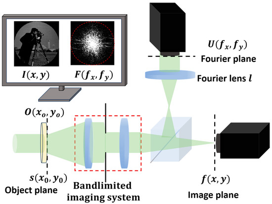
Figure 1.
Optical scheme of BIFT phase imaging method.
When the object with the complexed-valued response function was imaged, the object field was projected to the image plane and can be given by [26]
Then, the field was further Fourier transformed to the Fourier plane by a Fourier lens; the field at the Fourier plane can be given by
where (x, y) and (fx, fy) represent the two-dimensional spatial and spatial frequency coordinates, S1 is the finite size of illumination, h(x, y) is the point spread function (PSF) in image space as , where is the pupil function of the objective (numerical aperture NA, magnification M) with cut-off spatial angular frequency.
fc = NA/λ. Thus, the corresponding bandlimited image and the Fourier intensities were recorded, where the * donates the complex conjugate operation. With the recorded bandlimited image and its Fourier intensity and , the optical fields in image space and in Fourier space can be recovered with the BIFT algorithm [25].
The BIFT algorithm has been modified based on the HIO algorithm for two intensities measurements [44] by applying the intrinsic band limit constraint of finite aperture to remove the non-trivial ambiguities and combining the recorded intensities constraint to remove the trivial ambiguities [26]. The specific modifications in the j-th iteration are: (1) The estimated is imposed to the recorded image intensity, which is given by
where is the inverse Fourier transform of in the j-th iteration. (2) The feedback of the estimated is added in Fourier space to strengthen the band limit constraint that
where and are the optical field of the input and output in Fourier space in the j-th iteration, the is the amplified pupil function at the recording Fourier plane, and the is given by
Using this BIFT algorithm, the optical fields and can be retrieved with improved and fast convergence. Finally, the response function of object was given by dividing the magnification of the objective from .
2.2. The Super-Resolution BIFT Imaging by Analytic Extrapolation
As BIFT’s uniqueness is guaranteed, the light field can be accurately reconstructed to the theoretical limit of the Cramer–Rao bound [26]. However, due to the cut-off effect of the objective lens, high spatial frequencies cannot be recovered, but only low spatial frequencies within the finite aperture . In the BIFT imaging method, an object O (x0, y0) is projected into the image plane by the band-limited imaging system. The wave field is the Fourier transform of the bounded object field with the finite FOV, and thus introducing additional constraints of analyticity. The analyticity indicates three properties as follows:
- 1
- The optical field exhibits continuous differentiability and can be extended indefinitely in the Fourier plane;
- 2
- Any point of the optical field can be expressed as the sum of each other points in the field. In other words, any point of the optical field is not independent from others;
- 3
- The entire function can be uniquely determined by its behavior within any arbitrarily small region. The unknown portion of the analytic function can be inferred from its analyticity in that small region.
For a more comprehensive description of analyticity in the BIFT system, we provide the following mathematical analyses. Using the Equations (1) and (2), the Fourier transform of is given by
where is the Fourier transform of and is the Fourier transform of the finite FOV of . Considering with the discrete sampling with sampling point . The Equation (7) can be rewritten as
As we can see in Equation (7), although the function is discrete, the Fourier transform of the finite-aperture FOV is continuously differentiable. Therefore, the convolved light field is also continuously differentiable. Such continuous differentiability of this complex function ensures that it satisfies the Cauchy-Riemann equations, thereby exhibiting analyticity. However, due to the cut-off effect of the objective lens , we can only obtain partial information about the analytic function within the finite aperture, which is . As a result, property 3 can be used to infer the whole object’s spatial frequency from the known part of . To better understand the principle of analytic continuation, the Taylor series expansion serves as a simple example. By using the Taylor equation, a one-dimensional case of can be expressed as
In Equation (8), due to the continuous derivatives of the analytic function, the function outside the finite aperture can be approximated by constructing a polynomial series with coefficients from multiple order derivatives at the point within the band-limited region. However, in practice, the spatial frequencies within the aperture are also sampled by the camera’s pixels. Calculating the derivative of a point using discrete difference operations introduces significant errors. Therefore, we use matrix-based methods to analyze the analytic extrapolation. Assuming the sampled point of , the Equation (7) can be rewritten as
After the discrete sampling, Equation (9) can be rewritten as simple matrix form as follows:
where and x are the vectorized spatial frequencies of and , respectively, and the matrix A is . Considering the size and x with the vector dimension of and , respectively, and the analytic extrapolation range is normally larger than the known spatial frequency range (), thus the dimension of x will be much larger than y and the Equation (10) is ill-posed. However, because we already know the object’s spatial frequency in the finite aperture as , we can separate into
where the is the spatial frequency to be recovered. And the responding matrix A in Equation (10) can be split into two parts:
In Equation (12), the is the vectored with the dimension of and the A’ is the responding row of the matrix A with the dimension of . In Equation (11), x’ can be solved by . It is worth noting that, for Equation (12) to have the unique solution, the numbers of the equation must be larger than the number of unknowns, and matrix A should be full-rank. Considering these constraints, the range of a single analytic extrapolation cannot be greater than twice the range of finite spatial frequency (). When treating the case of , an optimization problem can be employed to search for an approximate solution, which increases the extrapolation range but also reduces reconstruction accuracy.
3. Simulation Result
3.1. The Performance of the Analytic Extrapolation in the Noise-Free Condition
After the phase recovery by the BIFT algorithm, the optical field can be perfectly reconstructed. The recovered optical field in the Fourier plane can then be analytically extrapolated using the method described in Section 2.2. Given the range of the finite FOV and finite aperture, we calculated the oversampling ratio (OSR) for the optical field in the image plane and the Fourier plane, respectively. The OSR is defined as the practical sampling ratio relative to the Nyquist sampling ratio. To verify the performance of the analytic extrapolation super-resolution imaging, simulations were conducted. A United States Air Force (USAF) resolution target was simulated as the object function with the normalized absorbance 0 to 1 and the phase from to . Under the finite FOV and finite aperture constraints in the BIFT imaging system, the sampled amplitudes of the image plane and Fourier plane are shown in Figure 2.
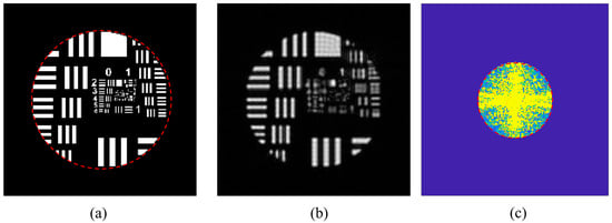
Figure 2.
The simulated object and sampled amplitude in the BIFT system. (a) The simulated object (red circle stands for the FOV of the BIFT system). (b) The diffraction-limited image. (c) The finite spatial frequency (red circle stands for the cut-off frequency).
Firstly, we evaluated the effect of the extrapolation range ratio (ERR), defined as the ratio of the number of pixels of the extrapolated field to the number of pixels in the range of finite spatial frequency (). To verify the final extrapolation error, an error function was calculated as follows:
where the is the optical field in the image plane after the extrapolation and is the ground truth of the field under the constraints of finite FOV, which has a high resolution. For a comprehensive comparison, we also calculated the error function of the band-limited optical field as follows:
We used Equations (13) and (14) to evaluate the relations between the ERR and the recovered , when the USAF target of Figure 2 was imaged. In the simulation, the OSR of 8 in the image plane was used to guarantee the uniqueness for different extrapolation ranges, and the results were evaluated for different OSRs in the Fourier plane. As shown in Figure 3, with the extrapolation range becoming larger, , were both increasing. As the ERR of 2, the is 0.0157, while it increases to 0.2883 as the ERR increases to 4. This error increasing comes from the matrix theory that we described in Section 2.2. When , the Equation (12) will have the unique solution (if it is full rank). Consequently, the extrapolation error will be small. However, when , the Equation (12) will have the multiple solutions, resulting in a significantly larger error. If we assume that an error of less than 0.1 is tolerable as a successful extrapolation, at this point, the extrapolation range is 2.5 times compared with the finite aperture range, which means that in the absence of noise, analytic extrapolation can achieve a 2.5-fold of SBP. This also implies that the resolution in the x and y directions will be improved by approximately times.
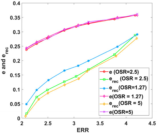
Figure 3.
Illustration of the error and with the function of EER at different OSRs of 1.27, 2.5, and 5 in the Fourier plane.
Apart from the impact of the extrapolation range on the accuracy of analytic extrapolation, the sampling rate in the Fourier plane also affects the reconstruction results. As shown in Figure 3, when the oversampling ratio in the Fourier plane is 1.25 and ERR = 2, the reconstruction error is 0.0488, which is higher than the reconstruction error at an OSR of 2.5. As the sampling rate further increases to 5, the reconstruction error becomes 0.00068. Although this is lower than the error at an oversampling ratio of 2.5 (0.00157), the reduction in error is not significant. This is because satisfying the Shannon sampling theorem typically requires the signal to be sampled at more than twice its rate. When the oversampling ratio is less than 2, discrete sampling can cause spectral aliasing, leading to signal distortion, which prevents accurate representation of the analytic function. When the oversampling ratio is greater than 2, the Shannon interpolation theorem can accurately recover the analytic function, and thus, further increasing the sampling rate does not result in a significant improvement.
To demonstrate the resolution improvement achieved by the analytic extrapolation method, we present the amplitude images of the diffraction-limited optical field, the analytically extrapolated field, and the ground truth shown in Figure 4. In Figure 4, Rows 1–3 correspond to ERR values of 2, 3, and 4, respectively. As shown in Figure 4, due to the cut-off effect of the finite aperture, the images in Figure 4(a1–c1) cannot display the details within the dashed line area. However, through analytic extrapolation, the structures within the dashed line area can be clearly resolved at different ERR values, as shown in Figure 4(a2–c2). As shown in Figure 4(a2,c2), at the ERR of 2, this area can be resolved and have the same value as the ground truth. At the ERR of 3, due to the range of the extension being larger, Figure 4(b2) has more detailed information in the rectangle area. In the red box, Figure 4(b2) clearly resolves the three lines in the resolution target, while Figure 4(a2) only resolves two lines. As ERR increases further to 4, the three lines in the red box become blurred again. This is because, despite the increased extrapolation range, the reconstruction error also increases, leading to a reduction in resolution.
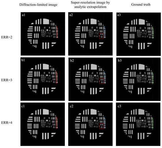
Figure 4.
The super-resolution ability by analytic extrapolation in the BIFT method; (a1–a3) the diffraction-limited image, super-resolution image, and ground truth at ERR of 2; (b1–b3) the diffraction-limited image, super-resolution image, and ground truth at ERR of 3; (c1–c3) the diffraction-limited image, super-resolution image, and ground truth at ERR of 4.
In order to clearly see how the improved resolution related to ERR and error, Figure 5 plots the area of the dashed line in detail, and the area of the purple box stands for the highest resolution area of dash line area. In Figure 5(a1), the analytic extrapolation can perfectly recover the structure of the dash line area and successfully resolve the three peaks of the USAF target at the area of purple boxes. However, for the bandlimited BIFT imaging, only one peak in the purple box can be resolved by the imaging system. With the ERR increasing to 3, the recovery error becomes larger than the threshold of successful analytic extrapolation. Even though our method can still resolve every peak of the USAF targets, the three peaks can still be distinguished in the purple box. In the purple box of Figure 5(a3), our method can still resolve the three peaks of the target but have a small contrast compared with the ground truth. Similarly, the resolution improvement is also evident in the phase images in Figure 5(b1–b3), the phase image at ERR of diffraction-limited, analytic extrapolation, and ground truth are shown in Figure 5(b1–b3), respectively (the red box area corresponds to the dashed line region in Figure 4 at ERR of 2). The super-resolution phase can be perfectly recovered by analytic extrapolation comparing with ground truth and successfully resolved three peaks with the phase delay from to compared with the traditional BIFT imaging method that can only distinguish one peak in Figure 5(b1).
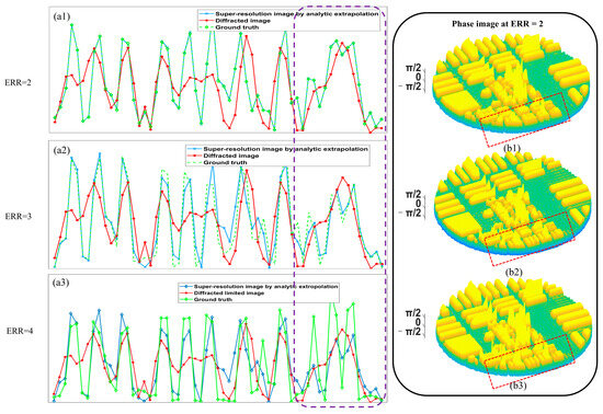
Figure 5.
The comparison of the amplitude and phase image among the analytic extrapolation, diffraction-limited, and ground truth. (a1–a3) The dashed line in Figure 4 with different ERRs. (b1–b3) The phase image of diffraction limitation, analytic extrapolation, and ground truth at ERR of 2.
3.2. Improving the Recovery from Noise by Analytic Extrapolation
Although the analytic extrapolation method performs well under noise-free conditions, it is sensitive to noise, which often leads to the failure of reconstructing high-resolution phase images. In this section, we analyze the impact of noise on analytic extrapolation using eigenvalue decomposition methods and address the noise issue through regularization to achieve high-resolution image reconstruction.
When exiting the noise in a finite spatial frequency area, the Equation (10) can be rewritten as,
where is the vector of noise and is the analytic extrapolation error introduced by the noise. The simple relation between the and can be given by
For a square matrix A, we can decompose it into eigenvalues and eigenvectors , which are also called eigenmodes, as follows (for non-square matrices, we can use the singular value decomposition):
Combining Equation (17), the Equation (16) can be rewritten as
Considering that Gaussian white noise is uniformly distributed in whole spatial frequency, and the eigenvectors are orthogonally normalized, the will have a similar value to . As a result, the key factor to affect the error of analytic extrapolation error is the eigenvalue . When the larger than 1, the will have a smaller value than , which means the noise can’t be amplificated by the analytic extrapolation. In contrast, when the much smaller than 1, the will have an especially larger value than , and the noise will dominate the analytic extrapolation process. Unfortunately, in the BIFT system, the matrix A’ often has an eigenvalue much smaller than 1, as shown in Figure 6.
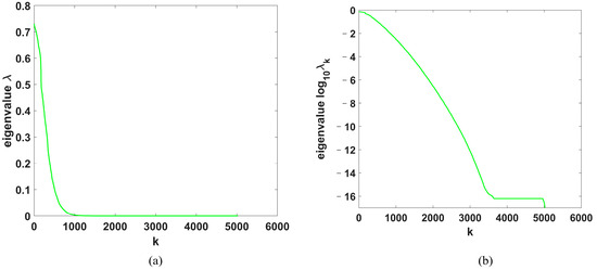
Figure 6.
(a) Illustration of the magnitude of eigenvalues of versus . (b) Illustration of the logarithm of eigenvalues of (a) versus k.
In Figure 6, the eigenvalues decrease rapidly as the number of k increases, indicating that higher-order eigenmodes passing through the band-limited system experience severe attenuation. This attenuation is exponential with increasing mode number, as demonstrated in Figure 6b. When higher-order patterns collected by the BIFT system are submerged in noise, they cannot be effectively recovered by the analytic extrapolation method. Consequently, the range of spatial frequencies that can be recovered through analytic extrapolation ultimately depends on the noise level.
To reduce the noise effect in the analytic extrapolation process, we added a small positive value to the small ensuring the noise is not amplificated too large in the recovery process. The selection of the value of the is depend on the signal to noise ratio. By the regulation of the , the super-resolution image can be recovered by analytic extrapolation under the noise corruption. Figure 7a illustrates , versus the varied (SNR) from 0 to 80 dB at the condition of ERR = 2. In Figure 7a, the , was decreased with the increase of SNR. When SNR < 10 dB, , have the same value, which means in this condition of SNR, the analytic extrapolation has little ability to expand the SBP. However, when SNR > 10, the decreases with respect to , which means that the resolution can be improved further increasing. However, even with the regulation, the reconstruction error still be higher than 0.1. To further reduce the error, it is beneficial to decrease the extrapolation range. Reducing the extrapolation range increases the number of equations relative to the number of unknowns in Equation (12), which reduces the ill-posedness of matrix A’, leading to more accurate reconstruction with lower error. Figure 7a shows the maximum extrapolation range (ERR) achievable when is less than 0.1. The maximum extrapolation range is roughly linearly proportional to the signal-to-noise ratio (SNR). At high SNR, regularization can increase the spatial bandwidth product by up to 1.8 times, corresponding to a resolution improvement of about 1.34 times. However, at low SNR, the analytic extrapolation only achieves a 1.3-fold increase in the spatial bandwidth product, resulting in a resolution improvement of approximately 1.15 times.
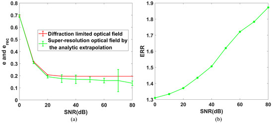
Figure 7.
(a) Illustration of the and with different SNRs at ERR = 2. (b) Illustration of the extrapolation range (ERR) changed with the SNR.
To verify the improvement of the resolution optical field, the real part of the recovered optical field, diffraction-limited optical field, and ground truth are given in Figure 8(a1–c1), respectively, at the SNR of 80 dB and ERR = 1.8. Figure 8(a2–c2) shows the magnified area in the red rectangle of Figure 8(a1–c1), respectively. The improvement of the resolution is obvious in the dashed line in Figure 8(a2,b2). However, this structure becomes blurred with the SNR decreasing, as shown in Figure 8(a3–c3) with the SNR of 20, 40, and 60 dB, respectively.
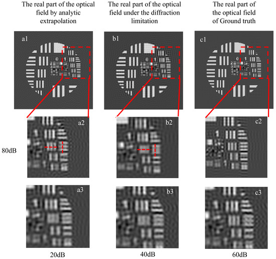
Figure 8.
The improvement of resolution by analytic extrapolation with different SNR. (a1–c1) The real part of the optical field by analytic extrapolation, diffraction-limited, and ground truth. (a2–c2) The magnified red rectangle area of (a1–c1). (a3–c3) The magnified red rectangle area of (a1) with SNR of 20 dB, 40 dB, and 60 dB.
4. Conclusions
In summary, we have proposed a method for achieving single-shot super-resolution phase imaging through analytic extrapolation. This approach utilizes the analyticity of the Fourier transform within the finite field of view. By leveraging the characteristic that partial information of an analytic function can be used to infer the complete information, our method can extend the limited spatial bandwidth of the BIFT system. This method does not require any prior information about the object and achieves super-resolution phase reconstruction with a single exposure.
The mathematical theory and numerical simulations were carried out to investigate the relationship between the construction error of the light field after analytic extrapolation and three critical factors: extrapolation range, oversampling rate, and signal-to-noise ratio (SNR). Firstly, in the absence of noise, effective extrapolation requires the oversampling rate in the Fourier plane to be greater than 2. Secondly, the construction error is linearly increased with the increase of the extrapolation range. When the error is less than 1/10, the analytic extrapolation method can increase the space-bandwidth product (SBP) by about 2.5 times, which means the resolution will improve by approximately 1.58 times. Additionally, the SNR is the most crucial factor affecting the success of analytic extrapolation. The small eigenvalues can amplify noise during the extrapolation process, leading to the failure of extrapolation. To mitigate noise effects, a regularization method was employed. Using this method, we obtained a linear relationship between the extrapolation range and SNR. As SNR varies from 0 to 80 dB, the SBP can be extended by 1.3 to 1.8 times, corresponding to a resolution improvement of 1.15 to 1.34 times.
Our BIFT phase imaging method is fundamentally different from previous single-shot methods of using coherent diffraction imaging [9]. The key constraints of our method are the finite aperture and finite FOV, which exist in common imaging systems such as microscopy, photography, remote sensing, astronomical telescopes, etc. Therefore, our proposed super-resolution method can have a wide range of applications. Our previous work showed that the BIFT dual-plane measurement can guarantee the uniqueness of phase retrieval, and the finite aperture provides a fixed, tight support for the stable recovery algorithm to converge to a global minimum, avoiding the need for prior knowledge of the object. Compared with the traditional interferential phase imaging methods, such as off-axis holography, phase contrast microscopy, and differential interference contrast microscopy, the non-interference nature of the BIFT method allows the imaging system to be more stable from environmental interference. In addition, for the spatially separating with conjugate inversion ambiguity to achieve the single-shot, the SBP of the off-axis holography is severely reduced compared with the in-line system of BIFT. Beyond this, in this paper, the SBP can be enhanced further by analytic extrapolation.
Although the 1.58-fold resolution enhancement achieved by analytic extrapolation currently falls short compared to the 2-fold enhancement achieved by synthetic aperture techniques, we believe this method still holds significant potential. The key to improving analytic extrapolation capability is to enhance the distinguishability of the small eigenvalues of matrix A’. Currently, the overly small eigenvalues indicate that the high-order eigenmodes are severely attenuated. However, there still exist practical methods to allow the high-order eigenmodes to be detected with high SNR, which include the use of structured illumination, random modulation, speckle illumination and specific coding illumination. Additionally, to improve the SNR, partially coherent light illumination could be used to reduce speckle noise from coherent beams. Finally, due to the guaranteed uniqueness and super-resolution ability of BIFT using analytic extrapolation, synthetic BIFT can potentially reduce the redundant, overlapping areas, significantly decreasing the required acquisition time compared to traditional synthetic aperture techniques.
Author Contributions
Conceptualization, Z.W.; methodology, K.X. and Z.W.; validation, K.X. and Z.W.; writing—original draft preparation, K.X.; writing—review and editing, K.X. and Z.W.; project administration, Z.W.; funding acquisition, Z.W. All authors have read and agreed to the published version of the manuscript.
Funding
Science and Technology Commission of Shanghai Municipality (20DZ2210300).
Institutional Review Board Statement
Not applicable.
Informed Consent Statement
Not applicable.
Data Availability Statement
The data that support the findings of this study are available from the corresponding author upon reasonable request.
Conflicts of Interest
The authors declare no conflicts of interest.
References
- Millane, R.P. Phase retrieval in crystallography and optics. J. Opt. Soc. Am. A 1990, 7, 394–411. [Google Scholar] [CrossRef]
- Dainty, J.C.; Fienup, J.R. Phase retrieval and image reconstruction for astronomy. In Image Recovery Theory & Application; Academic Press: Cambridge, MA, USA, 1987. [Google Scholar]
- Nam, D.; Park, J.; Gallagher-Jones, M.; Kim, S.; Kim, S.; Kohmura, Y.; Naitow, H.; Kunishima, N.; Yoshida, T.; Ishikawa, T.; et al. Imaging Fully Hydrated Whole Cells by Coherent X-Ray Diffraction Microscopy. Phys. Rev. Lett. 2013, 110, 098103. [Google Scholar] [CrossRef]
- Park, Y.; Depeursinge, C.; Popescu, G. Quantitative phase imaging in biomedicine. Nat. Photonics 2018, 12, 578–589. [Google Scholar] [CrossRef]
- Tahara, T.; Quan, X.; Otani, R.; Takaki, Y.; Matoba, O. Digital holography and its multidimensional imaging applications: A review. Microscopy 2018, 67, 55–67. [Google Scholar] [CrossRef]
- Shechtman, Y.; Eldar, Y.C.; Cohen, O.; Chapman, H.N.; Miao, J.; Segev, M. Phase Retrieval with Application to Optical Imaging: A contemporary overview. IEEE Signal Process. Mag. 2015, 32, 87–109. [Google Scholar] [CrossRef]
- Zernike, F. Phase contrast, a new method for the microscopic observation of transparent objects part II. Physica 1942, 9, 974–986. [Google Scholar] [CrossRef]
- Gabor, D. A New Microscopic Principle. Nature 1948, 161, 777–778. [Google Scholar] [CrossRef]
- Miao, J.; Sayre, D.; Chapman, H.N. Phase retrieval from the magnitude of the Fourier transforms of nonperiodic objects. J. Opt. Soc. Am. A 1998, 15, 1662–1669. [Google Scholar] [CrossRef]
- Fienup, J.R. Reconstruction of a complex-valued object from the modulus of its Fourier transform using a support constraint. J. Opt. Soc. Am. A 1987, 4, 118–123. [Google Scholar] [CrossRef]
- Koren, G.; Polack, F.; Joyeux, D. Iterative algorithms for twin-image elimination in in-line holography using finite-support constraints. J. Opt. Soc. Am. A 1993, 10, 423–433. [Google Scholar] [CrossRef]
- Shechtman, Y.; Beck, A.; Eldar, Y.C. GESPAR: Efficient Phase Retrieval of Sparse Signals. IEEE Trans. Signal Process. 2014, 62, 928–938. [Google Scholar] [CrossRef]
- Denis, L.; Lorenz, D.; Thiébaut, E.; Fournier, C.; Trede, D. Inline hologram reconstruction with sparsity constraints. Opt. Lett. 2009, 34, 3475–3477. [Google Scholar] [CrossRef] [PubMed]
- Zhang, W.; Cao, L.; Brady, D.J.; Zhang, H.; Cang, J.; Zhang, H.; Jin, G. Twin-Image-Free Holography: A Compressive Sensing Approach. Phys. Rev. Lett. 2018, 121, 093902. [Google Scholar] [CrossRef] [PubMed]
- Beinert, R. Non-negativity constraints in the one-dimensional discrete-time phase retrieval problem. Inf. Inference J. IMA 2017, 6, 213–224. [Google Scholar] [CrossRef][Green Version]
- Beinert, R.; Plonka, G. Ambiguities in One-Dimensional Discrete Phase Retrieval from Fourier Magnitudes. J. Fourier Anal. Appl. 2015, 21, 1169–1198. [Google Scholar] [CrossRef]
- Yamaguchi, I.; Ida, T.; Yokota, M.; Yamashita, K. Surface shape measurement by phase-shifting digital holography with a wavelength shift. Appl. Opt. 2006, 45, 7610–7616. [Google Scholar] [CrossRef]
- Yamaguchi, I. Phase-Shifting Digital Holography. In Digital Holography and Three-Dimensional Display: Principles and Applications; Poon, T.-C., Ed.; Springer: Boston, MA, USA, 2006; pp. 145–171. [Google Scholar] [CrossRef]
- Yamaguchi, I.; Kato, J.-i.; Ohta, S. Surface Shape Measurement by Phase-Shifting Digital Holography. Opt. Rev. 2001, 8, 85–89. [Google Scholar] [CrossRef]
- Nakatsuji, T.; Matsushima, K. Free-viewpoint images captured using phase-shifting synthetic aperture digital holography. Appl. Opt. 2008, 47, D136–D143. [Google Scholar] [CrossRef]
- Popescu, G.; Deflores, L.P.; Vaughan, J.C.; Badizadegan, K.; Iwai, H.; Dasari, R.R.; Feld, M.S. Fourier phase microscopy for investigation of biological structures and dynamics. Opt. Lett. 2004, 29, 2503–2505. [Google Scholar] [CrossRef] [PubMed]
- Pedrini, G.; Osten, W.; Zhang, Y. Wave-front reconstruction from a sequence of interferograms recorded at different planes. Opt. Lett. 2005, 30, 833–835. [Google Scholar] [CrossRef]
- Rodenburg, J.M. Ptychography and Related Diffractive Imaging Methods. In Advances in Imaging and Electron Physics; Hawkes, Ed.; Elsevier: Amsterdam, The Netherlands, 2008; Volume 150, pp. 87–184. [Google Scholar]
- Zheng, G.; Horstmeyer, R.; Yang, C. Wide-field, high-resolution Fourier ptychographic microscopy. Nat. Photonics 2013, 7, 739–745. [Google Scholar] [CrossRef] [PubMed]
- Kong, X.; Xiao, K.; Wang, K.; Li, W.; Sun, J.; Wang, Z. Phase microscopy using band-limited image and its Fourier transform constraints. Opt. Lett. 2023, 48, 3251–3254. [Google Scholar] [CrossRef] [PubMed]
- Xiao, K.; Kong, X.; Wang, Z. Unique phase retrieval with a bandlimited image and its Fourier transformed constraints. J. Opt. Soc. Am. A 2023, 40, 2223–2239. [Google Scholar] [CrossRef]
- Neifeld, M.A. Information, resolution, and space–bandwidth product. Opt. Lett. 1998, 23, 1477–1479. [Google Scholar] [CrossRef]
- Peng, G.; Caojin, Y. Resolution enhancement of digital holographic microscopy via synthetic aperture: A review. Light Adv. Manuf. 2022, 3, 105–120. [Google Scholar] [CrossRef]
- Granero, L.; Micó, V.; Zalevsky, Z.; García, J. Superresolution imaging method using phase-shifting digital lensless Fourier holography. Opt. Express 2009, 17, 15008–15022. [Google Scholar] [CrossRef]
- Micó, V.; Ferreira, C.; García, J. Surpassing digital holography limits by lensless object scanning holography. Opt. Express 2012, 20, 9382–9395. [Google Scholar] [CrossRef]
- Li, D.; Shao, L.; Chen, B.-C.; Zhang, X.; Zhang, M.; Moses, B.; Milkie, D.E.; Beach, J.R.; Hammer, J.A.; Pasham, M.; et al. Extended-resolution structured illumination imaging of endocytic and cytoskeletal dynamics. Science 2015, 349, aab3500. [Google Scholar] [CrossRef]
- Chowdhury, S.; Eldridge, W.J.; Wax, A.; Izatt, J.A. Structured illumination multimodal 3D-resolved quantitative phase and fluorescence sub-diffraction microscopy. Biomed. Opt. Express 2017, 8, 2496–2518. [Google Scholar] [CrossRef] [PubMed]
- Bian, L.; Suo, J.; Situ, G.; Zheng, G.; Chen, F.; Dai, Q. Content adaptive illumination for Fourier ptychography. Opt. Lett. 2014, 39, 6648–6651. [Google Scholar] [CrossRef]
- Dong, S.; Shiradkar, R.; Nanda, P.; Zheng, G. Spectral multiplexing and coherent-state decomposition in Fourier ptychographic imaging. Biomed. Opt. Express 2014, 5, 1757–1767. [Google Scholar] [CrossRef] [PubMed]
- Tian, L.; Li, X.; Ramchandran, K.; Waller, L. Multiplexed coded illumination for Fourier Ptychography with an LED array microscope. Biomed. Opt. Express 2014, 5, 2376–2389. [Google Scholar] [CrossRef] [PubMed]
- He, X.; Liu, C.; Zhu, J. Single-shot Fourier ptychography based on diffractive beam splitting. Opt. Lett. 2018, 43, 214–217. [Google Scholar] [CrossRef] [PubMed]
- Lee, B.; Hong, J.-y.; Yoo, D.; Cho, J.; Jeong, Y.; Moon, S.; Lee, B. Single-shot phase retrieval via Fourier ptychographic microscopy. Optica 2018, 5, 976–983. [Google Scholar] [CrossRef]
- Sun, J.; Chen, Q.; Zhang, J.; Fan, Y.; Zuo, C. Single-shot quantitative phase microscopy based on color-multiplexed Fourier ptychography. Opt. Lett. 2018, 43, 3365–3368. [Google Scholar] [CrossRef]
- Romberg, J. Imaging via Compressive Sampling. IEEE Signal Process. Mag. 2008, 25, 14–20. [Google Scholar] [CrossRef]
- Candes, E.J.; Romberg, J.; Tao, T. Robust uncertainty principles: Exact signal reconstruction from highly incomplete frequency information. IEEE Trans. Inf. Theory 2006, 52, 489–509. [Google Scholar] [CrossRef]
- Brady, D.J.; Choi, K.; Marks, D.L.; Horisaki, R.; Lim, S. Compressive Holography. Opt. Express 2009, 17, 13040–13049. [Google Scholar] [CrossRef]
- Marchesini, S.; He, H.; Chapman, H.N.; Hau-Riege, S.P.; Noy, A.; Howells, M.R.; Weierstall, U.; Spence, J.C.H. X-ray image reconstruction from a diffraction pattern alone. Phys. Rev. B 2003, 68, 140101. [Google Scholar] [CrossRef]
- Harris, J.L. Diffraction and Resolving Power. J. Opt. Soc. Am. 1964, 54, 931–936. [Google Scholar] [CrossRef]
- Fienup, J.R. Reconstruction and Synthesis Applications of an Iterative Algorithm. Transform. Opt. Signal Process. 1984, 373, 147–160. [Google Scholar]


Disclaimer/Publisher’s Note: The statements, opinions and data contained in all publications are solely those of the individual author(s) and contributor(s) and not of MDPI and/or the editor(s). MDPI and/or the editor(s) disclaim responsibility for any injury to people or property resulting from any ideas, methods, instructions or products referred to in the content. |
© 2024 by the authors. Licensee MDPI, Basel, Switzerland. This article is an open access article distributed under the terms and conditions of the Creative Commons Attribution (CC BY) license (https://creativecommons.org/licenses/by/4.0/).