Evaluation of Spatial–Temporal Variations in Ecological Environment Quality in the Red Soil Region of Southern China: A Case Study of Changting County

Abstract

The evaluation of ecological environment quality (EEQ) is an important method to measure the quality of ecosystem services. Therefore, the EEQ of Changting County, located in the red soil region of southern China, was assessed by using the remote sensing ecological index (RSEI) based on Landsat images from 1995 to 2019, and its spatiotemporal variability was identified by using the Global Moran’s I index, standard deviational ellipse, and kernel density estimation. The results showed that, firstly, the EEQ degraded from 1995 to 2000, then improved from 2000 to 2019; secondly, the spatial distribution of the RSEI for each study year was not random and had a strong positive correlation; thirdly, the directional distributions of the RSEI for all the grades were almost in the direction of southwest to northeast, and the spatial discrete characteristics of the moderate- and good-grade areas were almost consistent from 1995 to 2019; fourthly, the kernel density distribution of the moderate- and good-grade EEQ was located in towns within the Tingjiang River Basin and in the surroundings of the study area, respectively. This study can help managers to better understand the spatial–temporal variations in the EEQ in the study area, supporting the government in formulating a better ecological restoration strategy.

1. Introduction

Ecological environment quality (EEQ) refers to the suitability of the ecological environment for humankind’s survival and sustainable development based on ecological theory, and its evaluation has gradually become a hot topic in the ecology field in recent years [1]. The evaluation of EEQ not only can indirectly reflect the quality of the services and products provided by the eco-environment but also has gradually become an essential component of eco-environment protection and restoration. Recently, many researchers have put forward relevant theories and methods to evaluate the eco-environment status on different spatiotemporal scales, including the indicator system method [2,3,4], ecological footprint method [5], and machine learning method [6,7], among others. The indicator system method is the most commonly used method and mainly evaluates the EEQ through analyzing the selected indicators related to the characteristics of the study area using one or more mathematical models. Among them, the remote sensing ecological index (RSEI) is one of the most prominent indicator systems and is established based on the greenness, wetness, dryness, and heat indicators obtained by GIS and RS techniques to evaluate the EEQ of the study area using principal component analysis (PCA) [4].

The RSEI model can be applied to administrative units at different spatial–temporal scales, such as countries [8], provinces [9], cities [10,11], urban agglomerations [12], and counties [13,14], to discuss the spatial distribution, change trend, driving force factors, etc., of the EEQ. Non-administrative units have also been examined; for example, because of the special status of nature reserves and basins in the ecosystem, the EEQs of Changbai Mountain Nature Reserve and Ebinur Lake Wetland National Nature Reserve in Xinjiang in China were evaluated based on the RSEI, respectively. The former reserve showed an improvement trend in the EEQ during the study period, where the greenness and wetness indicators had a positive effect on the EEQ, while the dryness and heat indicators exhibited the contrary. In the latter reserve, the overall quality of the eco-environment was ameliorated from 2007 to 2016, and the wetness index had the greatest effect on the EEQ. Compared with those in 2007 and 2016, there was a strong positive correlation within the spatial distribution of the RSEI in 2013 [15,16]. Similarly, considering the important role of the Yellow River and the Yangtze River in the economic development of China, RSEI evaluation models of the Yellow River Basin and the Jialing River (as an important branch of the Yangtze River) Basin were established and showed an improved trend during the study periods [17,18]. In addition, RSEI models can be applied in regions with a smaller spatial scale, such as in mining areas [19]. Based on established RSEI evaluation models, the driving force factors and the spatial aggregation characteristics of EEQ have also been further analyzed by scholars; these can not only directly display the spatial–temporal variations in the High–High and Low–Low clustering regions of the RSEI value but can also help us to grasp the cardinal driving force factors affecting the variability in the EEQ by using Geodetector, Moran’s I index, etc. [20,21].

Changting County is a typical representative of the red soil erosion zone of southern China and is one of the counties with the most serious soil erosion [22]. Since 1995, the rapid development of urbanization and industrialization has had a serious effect on the eco-environment. Although, after many years of soil erosion control, the eco-environment of the region had improved, the spatial–temporal variability in the EEQ in the region was still unknown for the period 1995 to 2019. Therefore, we assumed that the selected greenness, wetness, dryness, and heat indices could express most of the characteristics of the eco-environment. The aims of this study were to (1) establish an RSEI evaluation model of Changting County based on evaluation indicators generated from Landsat TM and OLI/TIR images from the period of 1995 to 2019; (2) assess the overall level of the eco-environment and analyze the change in the EEQ trend from 1995 to 2019; and (3) identify the change in the spatial–temporal distribution characteristics of the EEQ in each grade from 1995 to 2019. The results of this study can provide a reference for formulating regional ecological restoration policy.

2. Materials and Methods

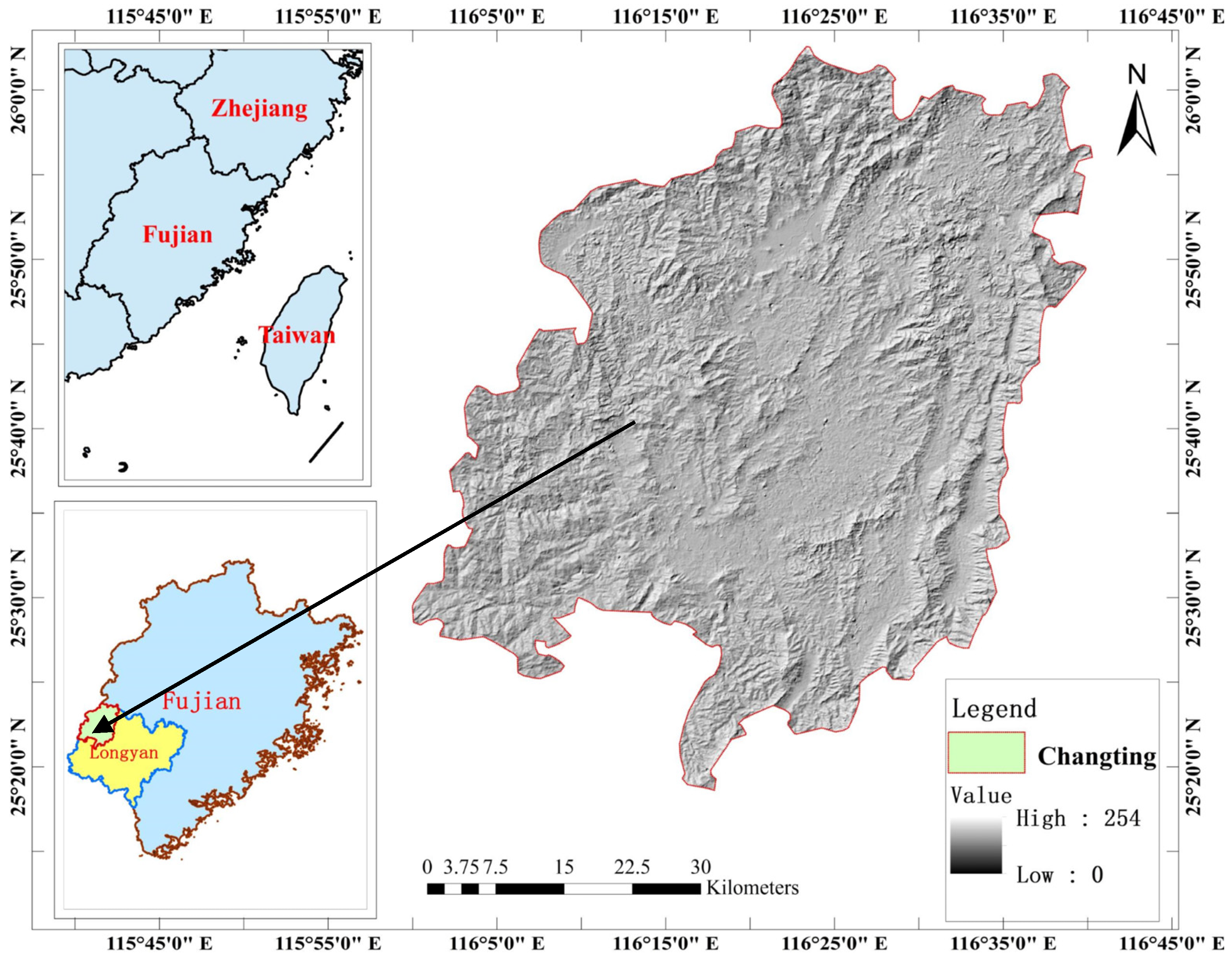
2.1. Overview of the Study Area

Changting County is located in the west of Longyan City, Fujian Province, China (25.31°~26.03° N, 116.01°~116.66° E), covering a total area of 3104.16 km² (Figure 1). The subtropical humid monsoon climate prevails in this area, with an average annual temperature of approximately 18.3 °C, an average annual precipitation of around 1700 mm, and an average annual frost-free period of about 260 d. The hilly landscape covers about 71% of the total area, with the highest elevation of 1459 m on Baisha Mountain, the lowest elevation of 238 m in the stream outlet of Tingjiang River, and an average elevation of 518 m. The forest coverage rate reaches 74% [23], and 79.8% of the soil covering area is dominated by red soil, which is strongly acidic and has poor water and fertilizer retention ability. The irrational exploitation of RE ores in the study area, one of the most important bases of rare earth (RE) resources in China, has led to the deterioration of the eco-environment, leading it to become one of the most serious areas of soil erosion in the red region of southern China. After nearly 25 years of effective control of soil erosion, the ecological environment has been greatly improved.

2.2. Methods

2.2.1. Data Sources and Processing

(1)

The vector data of the administrative boundaries of Changting County, Longyan City, and Fujian Province were provided by Fujian Provincial Geographical Information Center located in Fuzhou City, Fujian Province, China.

(2)

Landsat images from 1995–2019 were downloaded from the “Geospatial Data Cloud Website “http://www.gscloud.cn/” (accessed on 5 July 2023)” (

Table 1. The Landsat images used in this study.

Year	Acquired Date	Sensor Type	Path/Row	Cloud Cover
1995	7 December 1995	TM5	121/42	0.00%
2000	27 January 2000	ETM7	121/42	0.00%
2010	14 January 2010	TM5	121/42	0.00%
2019	23 January 2019	OLI/TIRS	121/42	2.29%

) to generate the evaluation indicators.

(3)

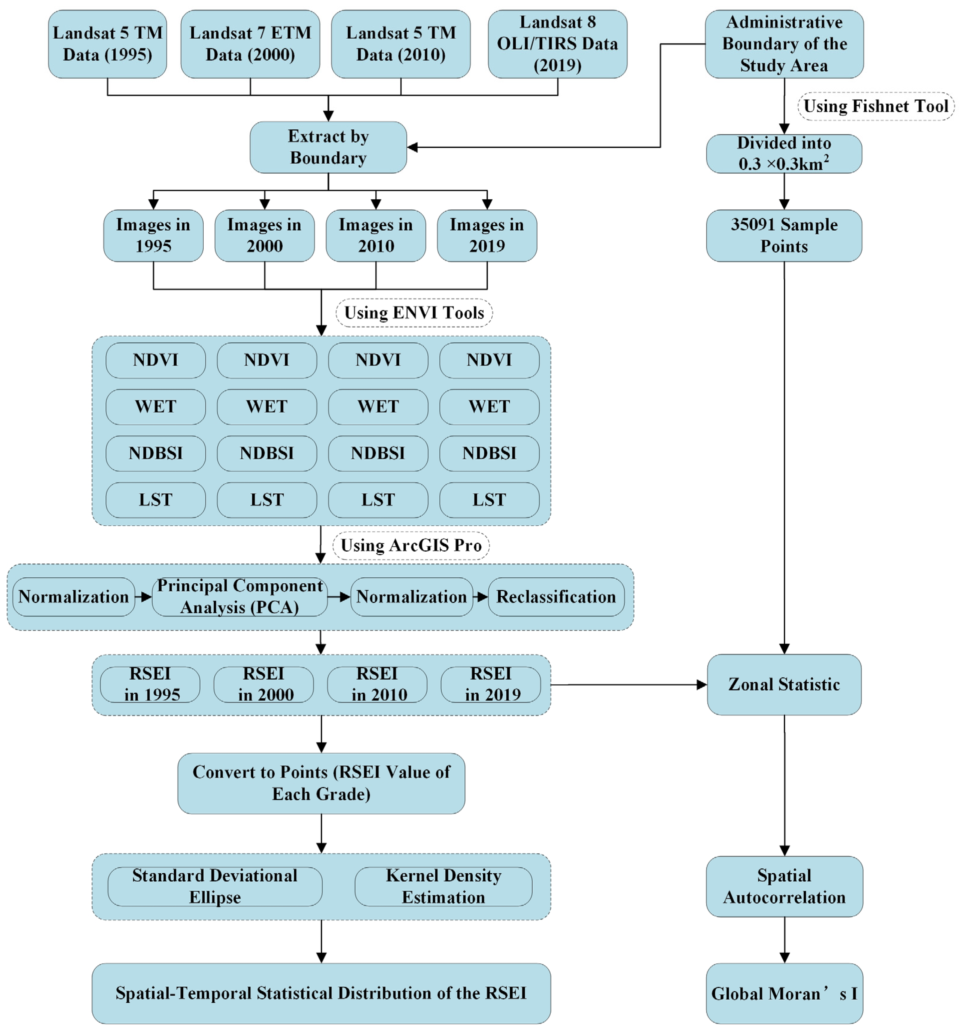
The study area was divided into a 0.3 × 0.3 km² grid to generate 35,091 sample points which were used to analyze the spatial autocorrelation characteristics combined with the RSEI.

(4)

As shown in Figure 2, the evaluation indicators, the RSEI, and the sample points were generated using ArcGIS Pro 3.2 and ENVI 5.3 software, which were used to further analyze the spatial–temporal distribution characteristics.

2.2.2. Indicators Used in the RSEI

In accordance with the literature [4], the normalized differential vegetation index (NDVI) representing the greenness index, the wetness component (WET) generated via Tassel Cap Transformation representing the wetness index, the normalized differential build-up and soil index (NDBSI) composed of the index-based built-up index (IBI) and the soil index (SI) as an indicator of dryness, and land surface temperature (LST) representing the heat index were selected as the evaluation indicators to establish the RSEI evaluation model and to assess the EEQ of the study area using PCA. Then, the EEQ of the study area was classified into 5 grades of worse (0.0–0.2), poor (0.2–0.4), moderate (0.4–0.6), good (0.6–0.8), and excellent (0.8–1.0) using the Natural Breaks (Jenks) method. The primary calculation formulas are presented in Equations (1)–(9). In these equations, PC1 denotes the first principal component of PCA, and b_blue, b_green, b_red, b_NIR, b_SWIR1, and b_SWIR2 are the reflectance of the blue, green, red, near-infrared, short-wave infrared 1, and short-wave infrared 2 bands of the TM and OLI sensors, respectively.

$$RSEI={f\left(NDVI,WET,LST,NDBSI\right)}_{PC1},$$

(1)

(1)

NDVI

NDVI can directly reflect the vegetation status in the study area. The calculation method is as shown in Equation (2) [24].

$$NDVI=\left(b_{NIR}-b_{red}\right)/\left(b_{NIR}+b_{red}\right),$$

(2)

(2)

WET

The WET index generated via Tassel Cap Transformation can directly reflect the humidity conditions of vegetation and soil and is calculated by Equation (3) [25,26]:

$$WET=c_1{b}_{blue}+c_2{b}_{green}+c_3{b}_{red}+c_4{b}_{NIR}-c_5{b}_{SWIR1}-c_6{b}_{SWIR2},$$

(3)

where, for TM sensors, c₁–c₆ are 0.0315, 0.2021, 0.3102, 0.1594, −0.6806, and −0.6109, respectively, and for OLI sensors, c₁–c₆ are 0.1511, 0.1973, 0.3283, 0.3407, −0.7117, and −0.4559, respectively.

(3)

NDBSI

NDBSI is characterized by the bare soil index and the index-based built-up index, expressed by Equations (4)–(6).

$$NDBSI=\left(IBI+SI\right)/2 ,$$

(4)

$$SI=\left[\left(b_{SWIR1}+b_{red}\right)-\left(b_{blue}+b_{NIR}\right)\right]/\left[\left(b_{SWIR1}+b_{red}\right)+\left(b_{blue}+b_{NIR}\right)\right],$$

(5)

$$IBI={\displaystyle \frac{\left\{\frac{{2b}_{SWIR1}}{\left(b_{SWIR1}+b_{NIR}\right)}\right.-\left.\left[\frac{b_{NIR}}{b_{NIR}+b_{red}}+\frac{b_{green}}{b_{green}+b_{SWIR1}}\right]\right\}}{\left\{\frac{{2b}_{SWIR1}}{\left(b_{SWIR1}+b_{NIR}\right)}\right.+\left.\left[\frac{b_{NIR}}{b_{NIR}+b_{red}}+\frac{b_{green}}{b_{green}+b_{SWIR1}}\right]\right\}}},$$

(6)

(4)

LST

The mono-window algorithm was used for the inversion of the land surface temperature, as shown in Equations (7)–(9) [27,28]:

$$T_s=\left[a\left(1-C-D\right)+\left(b\left(1-\mathrm{C}-D\right)+C+D\right)T_{sensor}-D{T}_a\right]/C,$$

(7)

$$C=\epsilon \tau ,$$

(8)

$$D=\left(1-\tau \right)\left[1+(1-\epsilon )\tau \right],$$

(9)

where a and b are −67.35535 and 0.458608 for TM/ETM+ sensors, respectively, but for OLI/TIRS sensors, they are −60.919 and 0.428, respectively; T_sensor is the brightness temperature value of the thermal infrared band; Ta represents the effective average atmospheric temperature; C and D can be calculated by Equations (8) and (9); ε is the surface emissivity ratio; and τ is the atmospheric transmittance of the thermal infrared band, which can be generated using the NASA website “http://atmcorr.gsfc.nasa.gov” (accessed on 11 July 2023) by inputting the imagery date and the central latitude and longitude values of the images. Because of the limitation of imagery dates on the NASA website, the ε and τ values for images in 1995 cannot be obtained; they can only be replaced by the values for images in 2000.

2.2.3. Analysis of Spatial Distribution Characteristics

Table 2. Analysis methodology.

Method Name	Formula	Meaning
Global Moran’s I	$I_G={\displaystyle \frac{n\sum _{i=1}^n\sum _{j=1}^n{\omega }_{i,j}\left(x_i-\overline{X}\right)\left(x_j-\overline{X}\right)}{\sum _{i=1}^n\sum _{j=1}^n{\omega }_{i,j}\sum _{i=1}^n\left(x_i-\overline{X}\right)}}$	$n \mathrm{is} \mathrm{the} \mathrm{total} \mathrm{number} \mathrm{of} \mathrm{elements};{ x}_i$$\mathrm{and} x_j$$\mathrm{are} \mathrm{the} \mathrm{property} \mathrm{values} \mathrm{of} \mathrm{elements} i \mathrm{and} j; \overline{X}$$\mathrm{is} \mathrm{the} \mathrm{average} \mathrm{value}; {\omega }_{i,j}$ is the spatial weight between elements i and j.
Standard Deviational Ellipse	$C={\displaystyle \frac{1}{n}}\left(\begin{array}{cc}{\sum }_{i=0}^n{\left(x_i-\overline{x}\right)}^2& {\sum }_{i=0}^n\left(x_i-\overline{x}\right)\left(y_i-\overline{y}\right)\\ {\sum }_{i=0}^n\left(x_i-\overline{x}\right)\left(y_i-\overline{y}\right)& {\sum }_{i=0}^n{\left(y_i-\overline{y}\right)}^2\end{array}\right)$	$n \mathrm{is} \mathrm{the} \mathrm{total} \mathrm{number} \mathrm{of} \mathrm{elements}; x_i$$\mathrm{and} y_i$$\mathrm{are} \mathrm{the} \mathrm{coordinates} \mathrm{of} \mathrm{element} i; \overline{x}$$\mathrm{and} \overline{y}$ are the coordinates of the mean center point of all the elements.
Kernel Density Estimation	$f\left(x,y\right)={\displaystyle \frac{1}{{nh}^2}}{\sum }_{i=0}^{n}k\left({\displaystyle \frac{d_i}{n}}\right)$	n is the total number of elements; k is the kernel function; di is the distance between element i and point (x, y); h is the smoothing bandwidth.

shows the principles of all the analysis methods used in the study in detail. Global Moran’s I can measure the spatial autocorrelation among geographical features based on the location and attribution values of each feature [29] and was therefore used to present the level of spatial autocorrelation of the EEQ in the study area. The standard deviational ellipse can express the central tendency, dispersion, and directional trends of geographical features [30] and was therefore used to reveal the spatial dispersion characteristics of the RSEI values in each grade. Kernel density estimation is a non-parametric statistical method that was used to discriminate the distribution of the density of the RSEI values in each grade [31].

3. Results

3.1. The Variations in EEQ

Table 3. Results of PCA.

Year	Indicators	PC1	PC2	PC3	PC4
2019	NDVI	0.64257	0.42440	0.61273	0.17764
	WET	0.37449	0.04581	−0.62275	0.68549
	LST	−0.43786	0.88361	−0.16250	0.03334
	NDBSI	−0.50512	−0.19257	0.45862	0.70529
	Eigenvalue	0.00706	0.00223	0.00091	0.00009
	Percent eigenvalue	68.6252	21.6641	8.8444	0.8663
2010	NDVI	0.68931	0.42277	0.57451	0.12671
	WET	0.18434	−0.04244	−0.38881	0.90169
	LST	−0.46812	0.87289	−0.10121	0.09315
	NDBSI	−0.52128	−0.23985	0.71311	0.40277
	Eigenvalue	0.00709	0.00221	0.00063	0.00009
	Percent eigenvalue	70.7658	22.0556	6.2941	0.8845
2000	NDVI	0.51739	0.74926	−0.18456	0.36993
	WET	0.38822	−0.39166	0.61905	0.55917
	LST	−0.62747	0.50178	0.57647	0.14891
	NDBSI	−0.43344	−0.18284	−0.50039	0.72685
	Eigenvalue	0.01318	0.00217	0.00149	0.00040
	Percent eigenvalue	76.4586	12.5904	8.6319	2.3190
1995	NDVI	0.72551	−0.13755	0.67359	−0.03147
	WET	0.22259	0.00488	−0.19411	0.95538
	LST	−0.32395	0.77371	0.51515	0.17619
	NDBSI	−0.56493	−0.61184	0.49317	0.23498
	Eigenvalue	0.00876	0.00152	0.00108	0.00023
	Percent eigenvalue	75.5732	13.1416	9.3369	1.9483

lists the contribution rates, eigenvalues, and percentages of each principal component (PC1–PC4) from 1995 to 2019. As depicted in Table 3, the contribution rate of the first principal component (PC1) was notably high, at 75.5732%, 76.4586%, 70.7658%, and 68.6252% for the periods of 1995, 2000, 2010, and 2019, respectively. This indicates that PC1, with the majority of the characteristics of the evaluation indicators, could be suitable for calculating the RSEI value of the study area. Within PC1, the coefficients of NDVI and WET were positive, while those of LST and NDBSI were negative, indicating that NDVI and WET had a positive correlation with the EEQ, whereas LST and NDBSI exerted a negative influence on the EEQ. Based on the absolute values of the index coefficients in PC1, NDVI had the greatest effect on the EEQ in 1995, 2010, and 2019, which was consistent with the high vegetation coverage of the study area. In contrast, in 2000, LST was the most prominent factor affecting the EEQ. This is mainly because the study area experienced rapid industrialization and urbanization after 1995, which had a significant effect on the eco-environment by intensifying the urban heat-island effect. Among the four indicators, WET had the least influence on the EEQ.

Table 4. Area and percentage of each grade.

Year	Average Value of RSEI	Worse		Poor		Moderate		Good		Excellent
		Area (km2)	Percent (%)	Area (km2)	Percent (%)	Area (km2)	Percent (%)	Area (km2)	Percent (%)	Area (km2)	Percent (%)
2019	0.672	0.04	0.001	41.92	1.35	485.87	15.66	2566.67	82.74	7.60	0.24
2010	0.613	0.47	0.02	73.75	2.38	1051.45	33.89	1971.83	63.56	4.59	0.15
2000	0.544	1.41	0.05	477.54	15.39	1435.49	46.28	1178.31	37.98	9.30	0.30
1995	0.683	0.08	0.003	1.38	0.04	639.17	20.61	2353.82	75.89	107.04	3.45

illustrates the RSEI average values and the area and percentage of each EEQ grade for the study area from 1995 to 2019. The data revealed that the RSEI average value during the study period was 0.628, indicating that the EEQ of the study area was generally in good condition. Initially, in 1995, the average value of RSEI was the highest (0.683); the value declined to 0.544 by 2000 and then rebounded to 0.672 by 2019. The data also showed a fluctuating trend in the EEQ, with an initial decline followed by an improvement from 1995 to 2000. The EEQ in most of the study area was categorized into the moderate and good grades, accounting for 98.4%, 97.45%, 84.26%, and 96.5% of the total area, respectively, in 2019, 2010, 2000, and 1995. These areas were predominantly distributed in mountainous regions, woodlands, and grasslands surrounding the city, exhibiting a certain degree of spatial continuity. Moreover, we found that the change trend for the moderate- and good-grade area was consistent with that for the average value of RSEI during the whole period. In contrast, the areas of other grades were very minimal, scattered in the north–central urban zones and some basins in the southwest (Figure 3); the change trend for these areas was inverse to that for the average value of RSEI, showing an initial increase followed by a decrease.

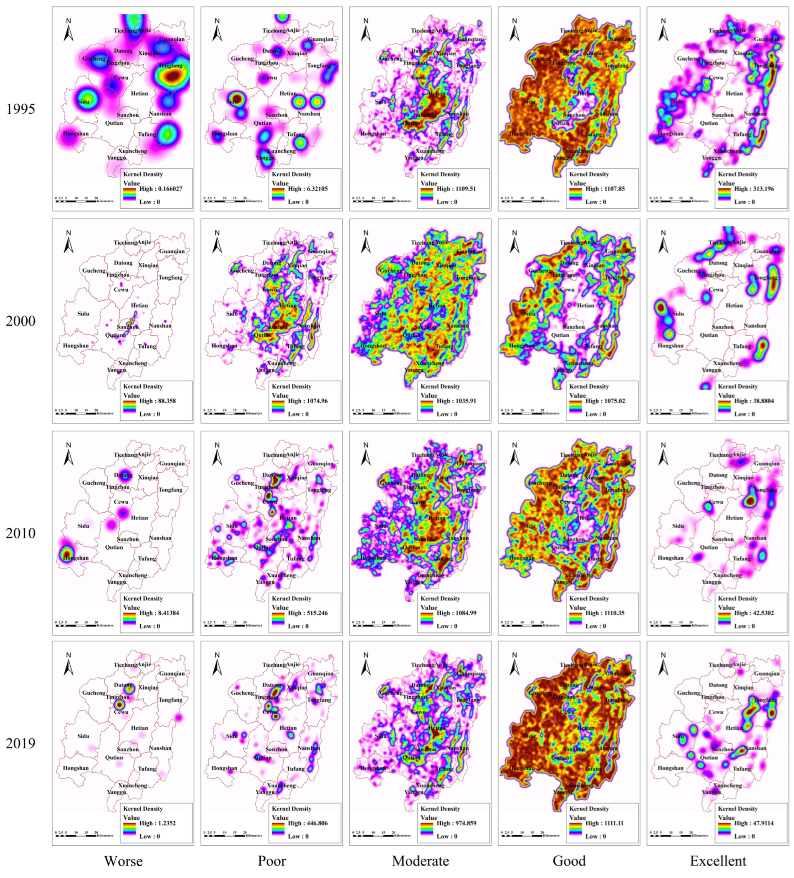
3.2. The Spatial Aggregation Characteristics of EEQ

The value of Global Moran’s I ranges from −1 to 1; if the value is less than 0, the spatial autocorrelation is negative, and the greater the value, the stronger the autocorrelation. If the z score is larger than 1.65, the spatial distribution of geographic elements is clustered. From 1995 to 2019, the Global Moran’s I values were 0.811, 0.818, 0.816, and 0.805 and the z scores were 213.707, 215.718, 214.982, and 212.191, respectively, indicating that the spatial distribution of EEQ not only was clustered but also had a strong positive autocorrelation. Therefore, kernel density estimation was employed to delve deeper into the spatial distribution characteristics of RSEI hot spots in each EEQ grade.

Table 5. Maximum value of kernel density of EEQ in each grade.

Grade	Year	Maximum Value of Kernel Density
Worse	1995	0.166
	2000	88.358
	2010	8.414
	2019	1.235
Poor	1995	6.321
	2000	1074.96
	2010	515.246
	2019	446.806
Moderate	1995	1109.51
	2000	1035.91
	2010	1084.99
	2019	974.859
Good	1995	1107.85
	2000	1075.02
	2010	1110.35
	2019	1111.11
Excellent	1995	313.196
	2000	38.88
	2010	42.53
	2019	47.911

presents the maximum kernel density values across different EEQ grades for the years 2019, 2010, 2000, and 1995. Notably, the maximum kernel density values in the moderate and good grades far outweighed those in other grades, indirectly reflecting that the majority of the study area was classified as moderate or good. Additionally, from 1995 to 2019, the change in the maximum kernel density values for the worse and poor grades followed a comparable trend, first increasing and then declining; this reinforced the observation that EEQ in the study area deteriorated until 2000 and then recovered by 2019.

Figure 4 delineates the spatial distribution of the kernel density for the EEQ, highlighting a multi-core pattern. Notably, the spatial distribution of the kernel density for the EEQ between the moderate and good grades showed a contrasting trend from 1995 to 2019. The spatial distribution of the kernel density for the moderate grade was notably located in the towns within Ting River Watershed, such as Datong, Tingzhou, Cewu, Hetian, and Sanzhou. Conversely, the spatial distribution of the kernel density for the good grade was observed in the peripheral areas surrounding the study area, predominantly covering the land use types of forests, woodlands, and so on.

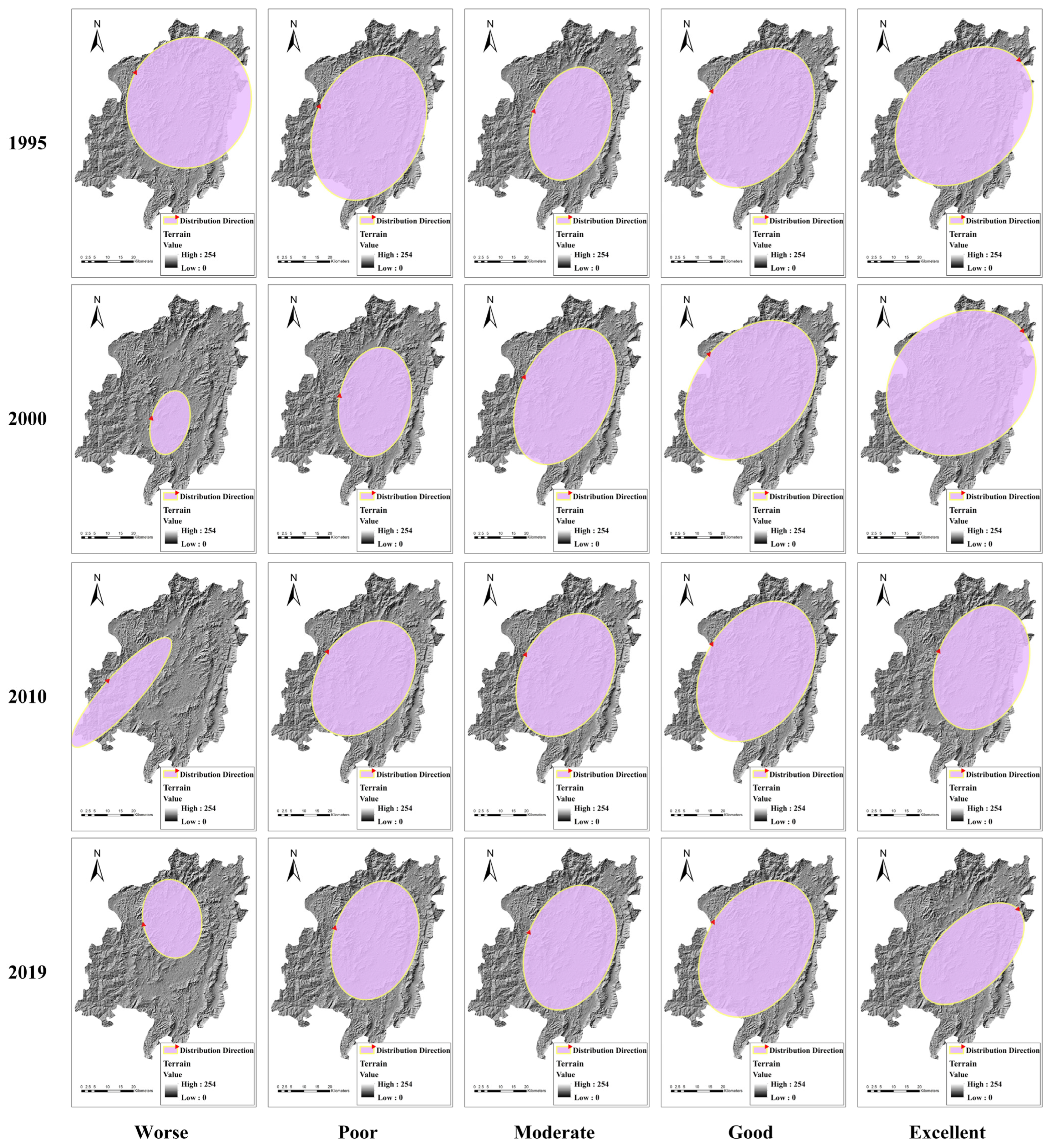
3.3. The Directional Distribution Characteristics of EEQ

As evidenced by

Table 6. Center, orientation, and ratio between x-axis and y-axis for EEQ in each grade.

Grade	Year	CenterX	CenterY	Orientation	Ratio
Worse	1995	443,469.590	2,848,187.638	29.786	1.077
	2000	436,175.418	2,831,295.446	14.422	1.685
	2010	417,453.093	2,834,374.896	42.459	4.003
	2019	437,002.909	2,853,162.378	169.679	1.337
Poor	1995	437,054.698	2,838,547.998	23.922	1.385
	2000	439,447.415	2,839,173.906	10.701	1.524
	2010	435,112.404	2,839,747.363	36.753	1.398
	2019	439,446.499	2,844,932.844	17.876	1.439
Moderate	1995	439,107.335	2,840,160.009	19.398	1.490
	2000	436,898.412	2,841,281.677	25.958	1.593
	2010	437,221.694	2,841,035.908	27.237	1.428
	2019	435,055.373	2,841,756.834	32.077	1.438
Good	1995	434,646.179	2,842,293.235	31.964	1.459
	2000	432,766.473	2,843,662.091	41.225	1.427
	2010	434,930.276	2,842,394.923	32.082	1.447
	2019	438,836.747	2,842,249.420	20.849	1.466
Excellent	1995	439,259.369	2,842,945.839	45.043	1.355
	2000	438,165.286	2,846,443.748	50.424	1.207
	2010	445,942.400	2,843,949.679	21.211	1.400
	2019	442,370.695	2,839,875.941	46.776	1.834

and Figure 5, the directional trend of the spatial distribution of the RSEI values for each grade was similar across the four periods, mainly orienting in a southwest–northeast direction. However, in 2019, a deviation was noted for the worse grade, with its distribution trending northwest–southeast. In 1995, the ratio of the worse grade was approximately equal to one, indicating a lack of pronounced clustering for the directional distribution in these areas. The central trends of the EEQ areas in the worse and poor grades varied across different study periods. Due to the scattered distribution of the EEQ areas in the worse grade, its central trend, directional trend, and discrete level were random from 1995 to 2019.

The center, orientation, and ratio of the moderate- and good-grade areas showed almost no obvious difference, suggesting that their central trend, directional trend, and discrete level adhered to a predictable spatial pattern. This underscored the dominant position of the areas of the moderate and good grades in the EEQ, which covered most of the study area. Conversely, the distribution centers of the excellent-grade areas, which were centered in the study area in 1995, experienced a southeastward shift, with the highest ratio observed in 2019. This indirectly indicated that the areas of excellent grade were small and had a scattered distribution within the study area.

4. Discussion

4.1. Spatial Correlations between Objects within Eco-Environments

Tobler’s First Law of Geography posits that all things are spatially related, with closer entities exhibiting stronger connections [32]. This principle underscores the importance of selecting an appropriate evaluation basic unit for EEQ, as it can significantly affect the assessment result. For example, the MW-RSEI evaluation model [19] considered the effect on the EEQ of the spatial correlation among things within a region by dividing the study area into multiple evaluation units, and the evaluation result was more detailed. Therefore, it is necessary to consider the influence of the basic evaluation unit on the EEQ.

However, many existing studies take the entire study area as an evaluation unit, neglecting the internal relations among features. To more accurately represent the ecological environment conditions, it is essential to consider the spatial components of the study area as evaluation units. For instance, evaluating the EEQ of one city based on each town as one separate evaluation unit can provide a more granular perspective. However, from the geographical standpoint, it may be advantageous to select sub-watershed units constituting the study area as the evaluation units, as this is more consistent with geographical processes. The quantity and shape of the sub-watersheds depend on the setting of the threshold of the drainage area. Reference [33] delved into the relationship between the lengths of drainage networks, different DEM resolutions, and drainage area thresholds to identify the optimal grid cell size and drainage area threshold for extracting the sub-watersheds of the study area. According to the results, it is vital to choose the appropriate DEM resolution and drainage threshold to evaluate the EEQ based on each sub-watershed as the evaluation unit.

4.2. Comprehensiveness and Complexity of EEQ Evaluation

In this study, we employed the PCA method integrating the selected four indicators (NDVI, WET, NDBSI, and LST) derived from Landsat images across four temporal snapshots (1995, 2000, 2010, and 2019) to evaluate the EEQ of the study area. The assessment results are almost coincident with the actual conditions and change trend of the eco-environment. Although the physical significance of the selected four indicators can reflect most of the characteristics of the effects of human activities and natural conditions on the eco-environment, these indices are not exhaustive in measuring the EEQ. The factors affecting the eco-environment encompass the topography, landscape, soil, climate, and social economy activity, among others. Therefore, it is necessary not only to consider the unique geographical traits of the study area but also to incorporate a broad spectrum of influencing factors.

For example, the ARSEI was established by integrating salinities and land degradation information to consider the unique characteristics of an arid area [34]. The EQEI was constructed based on 11 selected indicators, including the natural capital index (NCI), social pressure index (SPI), and economic support index (ESI) [35]. Additionally, factors such as slope [36], points of interest (POIs) [37], and land use [38,39] have been selected in other studies. Human interventions and shifts in natural conditions, including alterations in urban impervious surfaces [40], the construction of road networks [20], land consolidation [41], and events like floods, could cause dynamic changes in the EEQ. Therefore, an evaluation result at a fixed date cannot completely reflect the state of the eco-environment. It is essential to pay more attention to the effect of different time scales on the EEQ, such as various seasons or specific years, and a more comprehensive approach could ensure a more accurate representation of the ecological environment, providing a solid foundation for environmental policy and management decisions.

5. Conclusions

In our research, we built the RSEI evaluation model, evaluated the EEQ of the study area across four temporal benchmarks (1995, 2000, 2010, and 2019), and analyzed the spatial–temporal dynamics of the EEQ from 1995 to 2019. Based on the selected indicators (NDVI, WET, NDBSI, and LST), the evaluation results of the study area can almost reflect the actual conditions of the eco-environment. The key findings of this study can be summarized as follows:

(1)

The EEQ of the study area first declined and then recovered from 1995 to 2019. Most areas were of the moderate and good grades, and the overall level of the EEQ was good. NDVI and WET had a positive relation with the EEQ; the contrary was observed for LST and NDBSI.

(2)

The spatial distribution of EEQ was clustered rather than random, with a strong positive correlation. The spatial distribution of kernel density of the EEQ for each grade showed an obvious multi-core and multi-level pattern. In particular, the hot spots of kernel density of the moderate-grade areas were located in the towns within the Tingjiang River Basin, and those of the good-grade areas were distributed in the surroundings of the study area during the four periods (1995, 2000, 2010, and 2019).

(3)

The distribution of the EEQ areas for each grade was almost in a southwest–northeast direction. Compared with the distributions of other grade areas, the central trend, directional trend, and discrete level of the moderate- and good-grade areas were almost consistent.

These results can help managers to better understand the eco-status of the study area and to produce more comprehensive eco-environment protection and restoration policies.

References

1. Liu, P.; Ren, C.; Wang, Z.; Zhang, B.; Chen, L. Assessment of the eco-enviromental quality in the Nanweng River Nature Reserve, Northeast China by remote sensing. Chin. J. Appl. Ecol. 2018, 29, 3347–3356. [Google Scholar] [CrossRef]
2. Hu, X.; Xu, H. A New Remote Sensing Index for Assessing the Spatial Heterogeneity in Urban Ecological Quality: A Case from Fuzhou City, China. Ecol. Indic. 2018, 89, 11–21. [Google Scholar] [CrossRef]
3. Ma, H.; Shi, L. Assessment of Eco-Environmental Quality of Western Taiwan Straits Economic Zone. Env. Monit. Assess. 2016, 188, 311. [Google Scholar] [CrossRef] [PubMed]
4. Xu, H. A remote sensing urban ecological index and its application. Acta Ecol. Sin. 2013, 33, 7853–7862. [Google Scholar] [CrossRef]
5. Miao, C.; Sun, L.; Yang, L. The Studies of Ecological Environmental Quality Assessment in Anhui Province Based on Ecological Footprint. Ecol. Indic. 2016, 60, 879–883. [Google Scholar] [CrossRef]
6. Nourani, V.; Foroumandi, E.; Sharghi, E.; Dąbrowska, D. Ecological-Environmental Quality Estimation Using Remote Sensing and Combined Artificial Intelligence Techniques. J. Hydroinform. 2021, 23, 47–65. [Google Scholar] [CrossRef]
7. Shi, Z.; Li, H. Application of Artificial Neural Network Approach and Remotely Sensed Imagery for Regional Eco-Environmental Quality Evaluation. Env. Monit. Assess. 2007, 128, 217–229. [Google Scholar] [CrossRef]
8. Liao, W.; Jiang, W. Evaluation of the Spatiotemporal Variations in the Eco-Environmental Quality in China Based on the Remote Sensing Ecological Index. Remote Sens. 2020, 12, 2462. [Google Scholar] [CrossRef]
9. Gong, C.; Lyu, F.; Wang, Y. Spatiotemporal Change and Drivers of Ecosystem Quality in the Loess Plateau Based on RSEI: A Case Study of Shanxi, China. Ecol. Indic. 2023, 155, 111060. [Google Scholar] [CrossRef]
10. Gan, X.; Du, X.; Duan, C.; Peng, L. Evaluation of Ecological Environment Quality and Analysis of Influencing Factors in Wuhan City Based on RSEI. Sustainability 2024, 16, 5809. [Google Scholar] [CrossRef]
11. Yue, H.; Liu, Y.; Li, Y.; Lu, Y. Eco-Environmental Quality Assessment in China’s 35 Major Cities Based on Remote Sensing Ecological Index. IEEE Access 2019, 7, 51295–51311. [Google Scholar] [CrossRef]
12. Ji, J.; Wang, S.; Zhou, Y.; Liu, W.; Wang, L. Studying the Eco-Environmental Quality Variations of Jing-Jin-Ji Urban Agglomeration and Its Driving Factors in Different Ecosystem Service Regions from 2001 to 2015. IEEE Access 2020, 8, 154940–154952. [Google Scholar] [CrossRef]
13. Cheng, L.; Wang, Z.; Tian, S.; Liu, Y.; Sun, M.; Yang, Y. Evaluation of eco-environmental quality in Mentougou District of Beijing based on improved remote sensing ecological index. Chin. J. Ecol. 2021, 40, 1177–1185. [Google Scholar] [CrossRef]
14. Muhadaisi, A.; Zhang, F.; Liu, K.; Ayinuer, Y. Urban ecological environment evaluation based on Tiangong—2 and Landsat8 data. Remote Sens. Land Resour. 2020, 32, 209–218. [Google Scholar] [CrossRef]
15. Wang, S.; Zhang, X.; Zhu, T.; Yang, W.; Zhao, J. Assessment of ecological environment quality in the Changbai Mountain Nature Reserve based on remote sensing technology. Prog. Geogr. 2016, 35, 1269–1278. [Google Scholar] [CrossRef]
16. Jing, Y.; Zhang, F.; He, Y.; Kung, H.; Johnson, V.C.; Arikena, M. Assessment of Spatial and Temporal Variation of Ecological Environment Quality in Ebinur Lake Wetland National Nature Reserve, Xinjiang, China. Ecol. Indic. 2020, 110, 105874. [Google Scholar] [CrossRef]
17. Zhang, J.; Gu, Y.; Shen, J.; Cong, M.; Sun, Y.; He, J.; Yang, L. Analysis of Spatiotemporal Changes and Driving Factors of Ecological Environment Quality in the Yellow River Basin. Environ. Sci. 2024, 1–23. [Google Scholar] [CrossRef]
18. Wang, S.; Wu, W. Spatiotemporal Variation of Ecological Environmental Quality and Its Response to Different Driving Factors in Jialing River Basin in Recent 31 Years. Res. Soil Water Conserv. 2024, 31, 427–439. [Google Scholar] [CrossRef]
19. Zhu, D.; Chen, T.; Zhen, N.; Niu, R. Monitoring the Effects of Open-Pit Mining on the Eco-Environment Using a Moving Window-Based Remote Sensing Ecological Index. Env. Sci. Pollut. Res. 2020, 27, 15716–15728. [Google Scholar] [CrossRef]
20. Chen, X.; Zeng, X.; Zhao, C.; Qiu, R.; Zhang, L.; Hou, X.; Hu, X. The ecological effect of road network based on remote sensing ecological index: A case study of Fuzhou City, Fujian Province. Acta Ecol. Sin. 2021, 41, 4732–4745. [Google Scholar] [CrossRef]
21. Pariha, H.; Zan, M.; Alimjan, K. Remote sensing evaluation of ecological environment in Urumqi City and analysis of driving factors. Arid Zone Res. 2021, 38, 1484–1496. [Google Scholar] [CrossRef]
22. Deng, C.; Chen, Z.; Chen, H.; Chen, Z. Hyperspectral Estimation Models of Chlorophyll Content for Dicranopteris Dichotoma Leaves at Different Ecological Restoration Stages in the Eroded Red Soil Areas of Southern China. J. Geo-Inf. Sci. 2019, 21, 948–957. [Google Scholar] [CrossRef]
23. Jiang, T.; Xie, Y.; Chen, Z.; Chen, Z.; Chen, J. Reductions of Water Flow and Sediment Under Different Water Conservation Measures in Changting County of Fujian Province. Bull. Soil Water Conserv. 2018, 38, 35–41. [Google Scholar] [CrossRef]
24. An, Z.; XI, S. Analysis on the Evolution of Heat Island Effect and Its Influencing Factors in Ningbo Central City from 1990 to 2015. J. Hebei Univ. Eng. (Nat. Sci. Ed.) 2021, 38, 69–77. [Google Scholar]
25. Qin, Z.H.; Zhang, M.H.; Karnieli, A.; Berliner, P. Mono-Window Algorithm for Retrieving Land Surface Temperature from Landast TM6 Data. Acta Geogr. Sin. 2001, 56, 456–466. [Google Scholar]
26. Gong, J.; Xie, Y.; Zhao, C.; Gao, Y. Landscape ecological risk assessment and its spatiotemporal variation of the Bailongjiang watershed, Gansu. China Environ. Sci. 2014, 34, 2153–2160. [Google Scholar]
27. Zhao, L.; Zhao, Z. Projecting the Spatial Variation of Economic Based on the Specific Ellipses in China. Sci. Geogr. Sin. 2014, 34, 979–986. [Google Scholar] [CrossRef]
28. Wang, J.; Ma, J.; Xie, F.; Xu, X. Improvement of remote sensing ecological index in arid regions: Taking Ulan Buh Desert as an example. Chin. J. Appl. Ecol. 2020, 31, 3795–3804. [Google Scholar] [CrossRef]
29. Guo, Z.; Wei, W.; Zhang, X.; Li, Z.; Zhou, J.; Xie, B. Spatial distribution characteristics and influencing factors of eco-environmental quality based on RS and GIS in Shiyang River Basin, China. Chin. J. Appl. Ecol. 2019, 30, 3075–3086. [Google Scholar] [CrossRef]
30. Fu, J.; Cao, G.; Guo, W. Terrain Gradient Change of Land Use and Its Geographical Detector of Terrain Factors on the South-Facing Slope of Qilianshan Mountains from 1980 to 2018. Res. Soil Water Conserv. 2021, 28, 371–382. [Google Scholar] [CrossRef]
31. Ren, Y.; Zhou, T.; Li, H.; Xie, S.; Yin, Z. Research on the Urban Ecological Environment Pattern in the Main Urban Area of Chongqing Based on Remote Sensing and POI Data. Prog. Geophys. 2021, 36, 766–778. [Google Scholar] [CrossRef]
32. Wang, X.; Gong, W.; Huang, X.; Liu, T.; Zhou, Y.; Li, H. Assessment of Eco-Environmental Quality on Land Use and Land Cover Changes Using Remote Sensing and GIS: A Case Study of Miyun County. Nat. Environ. Pollut. Technol. 2018, 17, 739–746. [Google Scholar]
33. Xiong, Q.; Hong, Q.; Chen, W. Temporal and Spatial Response of Ecological Environmental Quality to Land Use Transfer in Nanling Mountain Region, China Based on RSEI: A Case Study of Longnan City. Land 2024, 13, 675. [Google Scholar] [CrossRef]
34. Wang, M.; Xu, H. Temporal and spatial changes of urban impervious surface and its influence on urban ecological quality: A comparison between Shanghai and New York. Chin. J. Appl. Ecol. 2018, 29, 3735–3746. [Google Scholar] [CrossRef]
35. Shan, W.; Jin, X.; Ren, J.; Wang, Y.; Xu, Z.; Fan, Y.; Gu, Z.; Hong, C.; Lin, J.; Zhou, Y. Ecological Environment Quality Assessment Based on Remote Sensing Data for Land Consolidation. J. Clean. Prod. 2019, 239, 118126. [Google Scholar] [CrossRef]
36. Fung, T.; Siu, W. Environmental quality and its changes, an analysis using NDVI. Int. J. Remote Sens. 2000, 21, 1011–1024. [Google Scholar] [CrossRef]
37. Baig, M.H.A.; Zhang, L.; Shuai, T.; Tong, Q. Derivation of a tasselled cap transformation based on Landsat 8 at-satellite reflectance. Remote Sens. Lett. 2014, 5, 423–431. [Google Scholar] [CrossRef]
38. Crist, E.P. A TM Tasseled Cap equivalent transformation for reflectance factor data—NASA Technical Reports Server (NTRS). Remote Sens. Environ. 1985, 17, 301–306. [Google Scholar] [CrossRef]
39. Wu, Y.; Wu, C.F.; Bei, H.L. Geographical distribution characteristics and mechanism of urban office buildings in Hangzhou during the transition period. J. Geogr. 2010, 65, 973–982. [Google Scholar]
40. Tobler, W.R. A computer model simulation of urban growth in the Detroit region. Econ. Geogr. 1970, 46 (Suppl. S1), 234–240. [Google Scholar] [CrossRef]
41. Chen, J.; Lin, G.; Yang, Z.; Chen, H. Parameters Optimization in Extracting Digital Drainage Networks with DEM. J. Geo-Inf. Sci. 2011, 13, 32–37. [Google Scholar] [CrossRef]
Figure 1. Geographical location of the study area.
Applsci 14 08641 g001
Figure 2. Methodology flow chart.
Applsci 14 08641 g002
Figure 3. Spatial distribution of the EEQ from 1995 to 2019.
Applsci 14 08641 g003
Figure 4. Change trend of kernel density of EEQ in each grade.
Applsci 14 08641 g004
Figure 5. Change trend of direction distribution of EEQ in each grade.
Applsci 14 08641 g005