Abstract
Due to the complex operating environment of LED lamp beads (hereinafter referred to as LED), the test method that only considers the action of multiple stresses alone ignores the mutual influence between stresses, making it difficult to accurately obtain the life indicators of LEDs, resulting in a large deviation in the theoretical life results. In this regard, this paper proposes a multi-stress accelerated degradation evaluation method considering generalized coupling and conducts an accelerated degradation test (ADT) to evaluate the life of LEDs. We identified three stress sources and designed five new high-gradient ADTs. Through experimental data, we found that the three stress sources are strongly coupled on this LED. Then, a generalized coupling maximum likelihood estimation method (MLE) for the entire sample was constructed, and the particle swarm algorithm was used to solve the parameters. Finally, the life of this LED was evaluated based on the experimental data. The results show that the life of the LED considering multiple-stress coupling is within 6.5% of the historical life scatter point, which is more in line with the actual working environment.
1. Introduction
With the advancement of LED lighting and display technology, LED products that ensure high efficiency and cost-effectiveness are gradually replacing traditional lamp beads in various application fields. However, as the reliability of LED chips continues to improve, the failure data generated by rated stress tests are becoming fewer and fewer, or even fault-free. It is necessary to adopt accelerated test methods to accelerate the product failure process while keeping the failure mechanism unchanged, reduce test time, and shorten the development progress. The failure mechanisms of LEDs are divided into three categories: the semiconductors, interconnects, and the package [1]. Failure mechanisms related to semiconductors include the generation and movement of defects and dislocations, et al. Interconnection-related failure mechanisms include wire breakage and wire ball bond fatigue induced by electrical overstress, et al. Encapsulation-related failure mechanisms include encapsulant, delamination, encapsulant yellowing, and lens cracking, et al. High current, poor assembly, and moisture intrusion can be classified as external causes of LED failure [2,3,4]. As reviewed in paper [1], light output degradation is the main failure mode of LEDs, which is caused by hydromechanical stress and electrical stress in addition to thermal stress.
The reliability of LED chips heavily depends on the conditions under which the system runs, in particular, the temperature and the humidity [5]; as a result, the traditional simple stress test cannot truly reproduce the actual working environment. Therefore, it is necessary to study the multi-stress accelerated life assessment method to accurately obtain the life data of LED chips in the actual use environment.
Currently, many scientists have conducted research on multi-stress acceleration models. Noguera deducted that temperature is the most significant factor affecting the life of LEDs, followed by humidity, but did not take into account its coupling effect [6]. Li combined the traditional acceleration model and proposed a dual-stress and triple-stress accelerated life model suitable for custom-circuit samples, electronic fuze, and smart electricity meters to predict reliability indicators [7]. Yang et al. proposed some reliability tests and evaluation methods for accelerated life tests and accelerated degradation test models [8,9,10]. Miao et al. studied the prediction of UV LED life, but they only considered the UV LED life test at room temperature, which lasted more than 8000 h. They did not consider the impact of the actual environment on the UV LED, and the error between the life and the actual value was quite large [11]. Liang designed a step-stress accelerated degradation test in the UV LED life test, with temperature and drive current as gradually increasing loads, and different failure mechanisms occurred in the test. The author did not consider the coupling of temperature and current in the test [12]. Ibrahim proposed a Bayesian approach to estimate the remaining useful life of high-power white light LED packages and lamps without considering the stress coupling relationship in the accelerated degradation test [13]. However, the use of multi-stress acceleration models ignores the mutual influence between stresses and does not consider the true correlation between stresses, resulting in a large deviation in the estimated life of the test.
Liu proposed a general multi-stress acceleration model considering generalized coupling, but only simulation data are available [14]. Although Zhang considered stress coupling, he directly concluded that humidity and current stress were not coupled based on expert experience [15]. In addition, there were fewer samples for different stress experiments, a smaller current stress interval, and a shorter test time, which resulted in the coupling of temperature, humidity, and current being ignored. To solve the above problems, a multi-stress accelerated life evaluation method considering generalized coupling is proposed. Based on the failure mechanism of LED, five stress-combination ADTs of three stress sources are redesigned. To determine the accuracy of life, this paper selects full-sample experiments and proposes a full-sample test maximum likelihood estimation (MLE) method for parameter estimation. The particle swarm algorithm is combined to solve the multi-stress generalized coupling accelerated model. The experimental data show that the temperature, humidity, and current are strongly coupled on this LED. The life distribution deviation considering the actual environmental stress coupling, ignoring the humidity–current coupling, and ignoring the stress coupling is discussed. The rest of this paper is organized as follows. The study’s detailed methodology is provided in Section 2. In Section 3, the results obtained, as well as inferences associated with the results, are described. Section 4 describes the obtained results and the inferences related to the results. Section 5 concludes this study.
2. Materials and Methods
2.1. Multi-Stress Acceleration Model Considering Generalized Coupling
2.1.1. Arrhenius-Based Multi-Stress Generalized Coupling Acceleration Model
The Arrhenius model originated in the field of chemistry and is widely used in accelerated test modeling in papers [11,12,16,17,18,19,20]. It is generally used to describe the relationship between the product life characteristic quantity and the applied temperature stress, which can be expressed as Equation (1).
where k(T) represents the life characteristics and is the product coefficient, which is a constant and is only related to its failure mechanism. is the activation energy of the chemical reaction, is the Boltzmann constant, and is the temperature stress in Kelvin temperature.
Equation (1) shows that life characteristics are positively correlated with chemical reaction speed. Since is a constant, for the sake of generalization, is abbreviated to and is abbreviated to ; that is, Equation (1) can be simplified to Equation (2).
where represents the effect of temperature on life and represents the influence coefficient of temperature.
Scientists studied the life-related model under dual stress, including temperature and voltage, as well as temperature and humidity, based on the traditional Arrhenius chemical model, as shown in Equation (3) [21,22,23,24,25].
where represents any non-temperature stress, represents other stress options such as humidity and current that may be coupled with temperature, and and are substitutes for unknowns in different material environments. Among them, can be simplified to . This formula can be simplified to Equation (4).
Similar to the dual-stress reaction rate model, the N stress reaction rate models based on the Arrhenius model will consist of single-stress coupling terms, dual-stress coupling terms, triple-stress coupling terms, quadruple-stress coupling terms, etc., where m stress coupling terms contain N stress coupling terms, a total of N terms, where m stress coupling terms contain elements, for example, the dual-stress coupling term will contain 3 elements, and the triple-stress coupling term will contain 9 elements. In summary, the above model can be expanded to N different stress life models, which are Equation (5):
represents N types of stress, such as temperature–humidity stress, and N stress triple-stress coupling terms, such as temperature–humidity–current stress, until all N stresses are coupled. Here, represents the unknown parameter of the model, and n > m is to ensure that the same term is not included in the consecutive multiplication terms. It should be noted that when , the second and subsequent multiplication terms do not exist in Equation (5), and the double-stress coupling term is represented by the last term in Equation (5). When , the third and subsequent multiplication terms do not exist in Equation (5), and the triple-stress coupling term is represented by the last term in Equation (5). That is, when , the i-th and subsequent multiplication terms do not exist in Equation (5), and the i-th stress coupling term is represented by the last term in Equation (5).
2.1.2. Prerequisites of the Model
A failure mode of LED is caused by N different stresses. For example, when is higher than normal use and storage pressure, can accelerate the aging process of the product. At this time, one or more stresses can be selected. The stress level setting of N accelerated stresses cannot change the failure mechanism of a product during accelerated degradation testing; that is, the failure mechanism of the LED in the accelerated life test of these accelerated stresses should be consistent with the failure mechanism of the LED during normal use. The model needs to meet the following three assumptions:
1. Under each stress level combination, n samples are randomly selected and put to the test for a certain period. Assume that the LED failure life is t; they are independent of each other and obey the Weibull distribution. Under the accelerated life test, the cumulative distribution function of the life is Equation (6).
where is the shape parameter and is the scale parameter. In LEDs, determines the trend of failure rate over time. When , it usually indicates degradation failure; that is, the failure rate will increase over time. When indicates early failure, and when , it means that the failure rate is constant and is not affected by time. represents the characteristic life; that is, at this point in time, 63.2% of the samples will fail. Under the action of various stress combinations, the degradation process of LEDs may accelerate, thereby changing . Under stresses of higher temperature, higher current, or high humidity, may increase, indicating that the failure rate of LEDs will rise faster over time, reflecting accelerated degradation failure; similarly, under stress combinations such as high temperature, high current, or high humidity tends to accelerate the degradation of LEDs, resulting in a decrease in , which reflects that LEDs are more likely to fail under these stresses. The effect of different stress combinations can be quantified by the change in : the higher the stress, the lower the value, which means that the LED has a shorter life under this stress combination.
Accelerated testing will cause the failure of the LEDs to occur earlier to a certain extent, while the exponential distribution of constant failure rate will lead to excessive deviation in the later stage. Therefore, the Weibull distribution with increasing failure rate over time is more suitable for LEDs [26,27].
2. In the test, the multi-stress and life satisfy a certain relationship, and it is necessary to ensure that the accelerated stress level does not exceed the maximum stress level that the LED can withstand. For the Weibull distribution, its characteristic life satisfies the multi-stress acceleration model in Equation (7).
where is the standardized multi-stress vector, , and is the standard mode of the stress , which can be expressed as Equation (8).
In the formula, is the stress normal stress level, and is the accelerated stress level.
Take the logarithm of both sides of equation X and standardize them according to Equation (8). The multi-stress acceleration model in which the life obeys the Weibull distribution under the combined action of three stresses is Equation (9), and the detailed calculation process is shown in Appendix A.
where in , , and represent the standardization of temperature, humidity, and current stress, respectively. The temperature here represents the Kelvin temperature. The Celsius temperature of subsequent tests needs to be converted to Kelvin by adding 273.
3. The failure mechanism of the LEDs must remain constant in the accelerated test at different selected stress levels; that is, is independent of .
If LEDs want to use the above model, the first assumption must be met; that is, it is necessary to determine whether the LED life under each stress obeys the Weibull distribution. Then, in the selection of test stress, it is necessary to ensure that the failure mechanism of the accelerated stress test is the same as the product’s historical failure mechanism at room temperature. Finally, in the accelerated test, it is necessary to ensure that the failure mechanism of LEDs under different stresses remains unchanged; that is, is independent of .
2.1.3. MLE Method for Full Samples
A full-sample test means that the test is stopped only when all samples fail. This type of test can obtain more complete data. The advantage is that the statistical analysis results are better, but the disadvantage is that it takes a long time. In a full-sample test, there are n test samples. The test is stopped when all devices fail at time tn. The failure time is recorded in order. The failure time before the test is stopped is t1 − tn, and the MLE is Equation (11):
Expanding to the case of multiple stresses, a total of q groups of multiple stress tests are designed. In the h group of tests, there are nh specimens, and the failure time can be expressed as th1, th2, …, thi, …, thn (h ≤ q). Therefore, under multiple stress combinations of h, the logarithmic probability function of the product failure Formula (12) is as follows:
Among them, ln ηh (α0, α1, …, αp) is the generalized coupled acceleration model under the hth group of stress combinations. After substituting the above formula into the multi-stress coupling model, the maximum likelihood function of all stress combinations of the complete sample is obtained as follows in Equation (13):
2.2. Accelerated Degradation Test
2.2.1. LED Failure Definition
There are two types of LED failures: accidental catastrophic failures and degradation failures. With the improvement of LED manufacturing technology, the proportion of accidental failures in LEDs has gradually decreased, and degradation failures are the main failure mode of LEDs today.
Light Output Performance (LOP) refers to the optical power that an optoelectronic component can output under a certain current. This concept is usually used to evaluate the performance of light-emitting diodes (LEDs). According to IEC International Electrotechnical Commission standards and relevant Chinese standards, when the light power of LED lighting decays to 70% of the rated light power, it is usually judged that the product has reached the end of its life. This standard is widely used to measure the performance and durability of LED lamps. Specifically, the time for the light power to decay to 70% (usually marked as L70) refers to the time required for the light output of an LED lamp to drop to 70% of its initial light output under specified conditions of use. This time is usually used to evaluate the service life of LED lamps. Since the initial brightness of LEDs is different, this article selects LEDs with similar initial brightness as a group, and LOP is judged to be 70% of its initial LOP. BE (Basic Error) is the deviation between the measured LOP and the initial LOP, defined as follows in Equation (14):
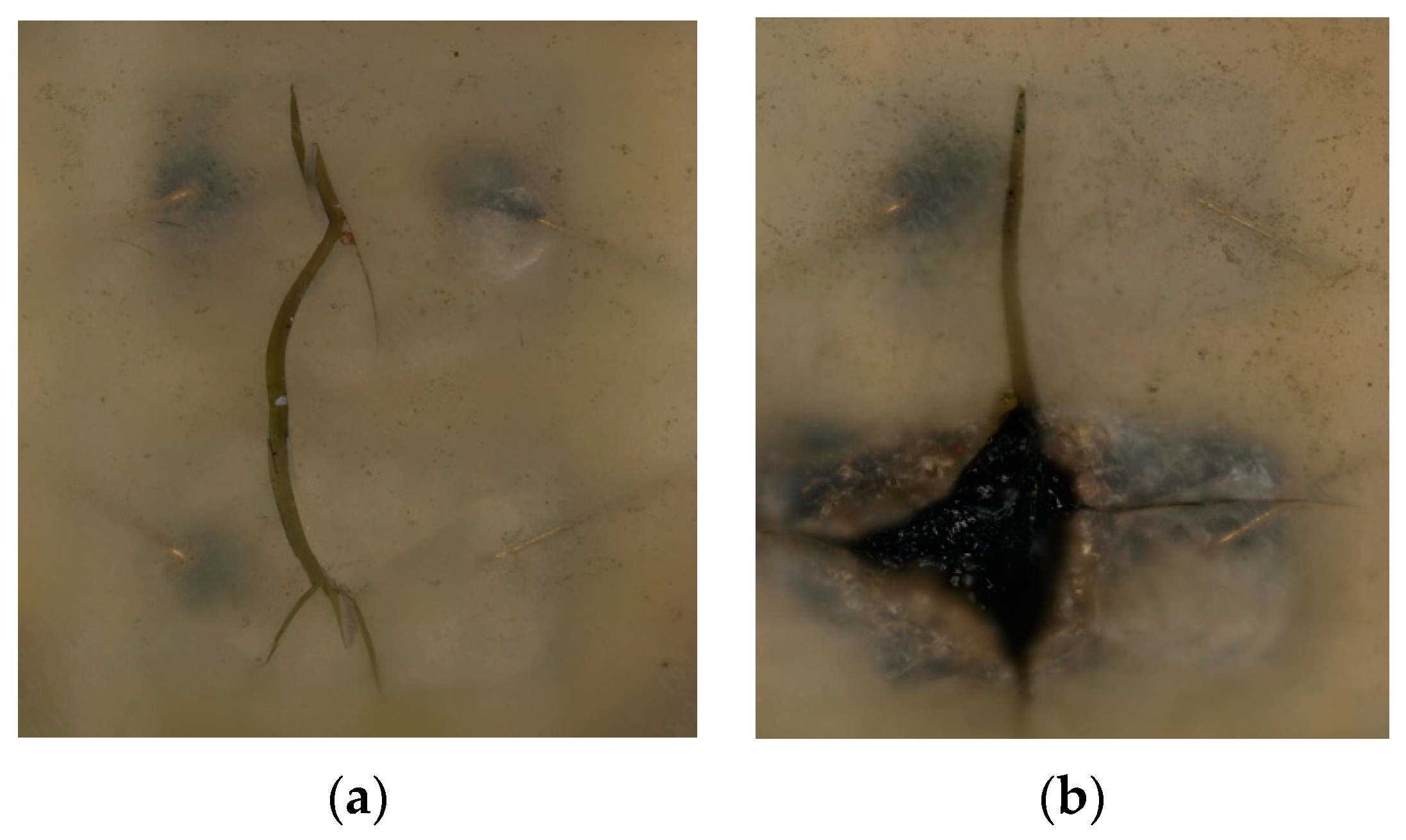
where is the initial light output performance indicating the initial value of a single LED before the test and is the testing light output performance indicating the value of one observation during the test. For example, under the conditions of 95 °C, 45% humidity, and 525 mA current, the initial LOP of the first LED in the first group of experiments was 510.5 mw, and it was 483.9 mw after 24 h of testing; that is, the rate of change in 24 h was −5%. The initial LOP values of the 10 LEDs in the first group of experiments were 510.5, 522.9, 527.1, 527.1, 506.3, 516.3, 530.4, 524.6, 522.1, and 522.1, with the maximum being 530.4 and the minimum being 506.3. The LOP attenuation of the 24 h test was compared with its initial LOP. The BE value is very important when judging LED failure. According to the L70 standard, the LED is declared failed when the difference between the LOP of the LEDs after degradation and the initial LOP of the LEDs accounts for −30% (−0.3) of the initial LOP of the LEDs. Many faults can cause LED LOP degradation, such as extreme thermal shocks that can break the dies of LEDs. The high electrical stress and extreme thermal shock are the causes of die cracking [28,29], as shown in Figure 1a,b. However, in many cases, the LED has no physical damage or burn marks. The life and performance of LEDs are limited by crystal defect formations in the epitaxial layer structure of the die [30]; electrostatic discharge (ESD) causes LED failure [31], etc. In this case, the cause of failure can only be seen after the test is completed and the sol is used under a microscope, such as in Figure 2.
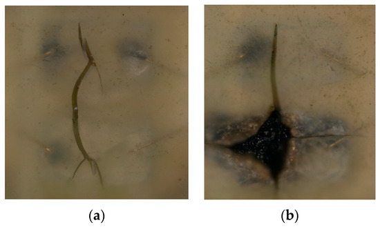
Figure 1.
Appearance of failed LEDs.
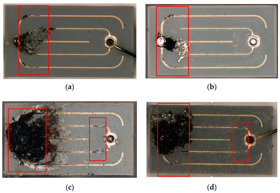
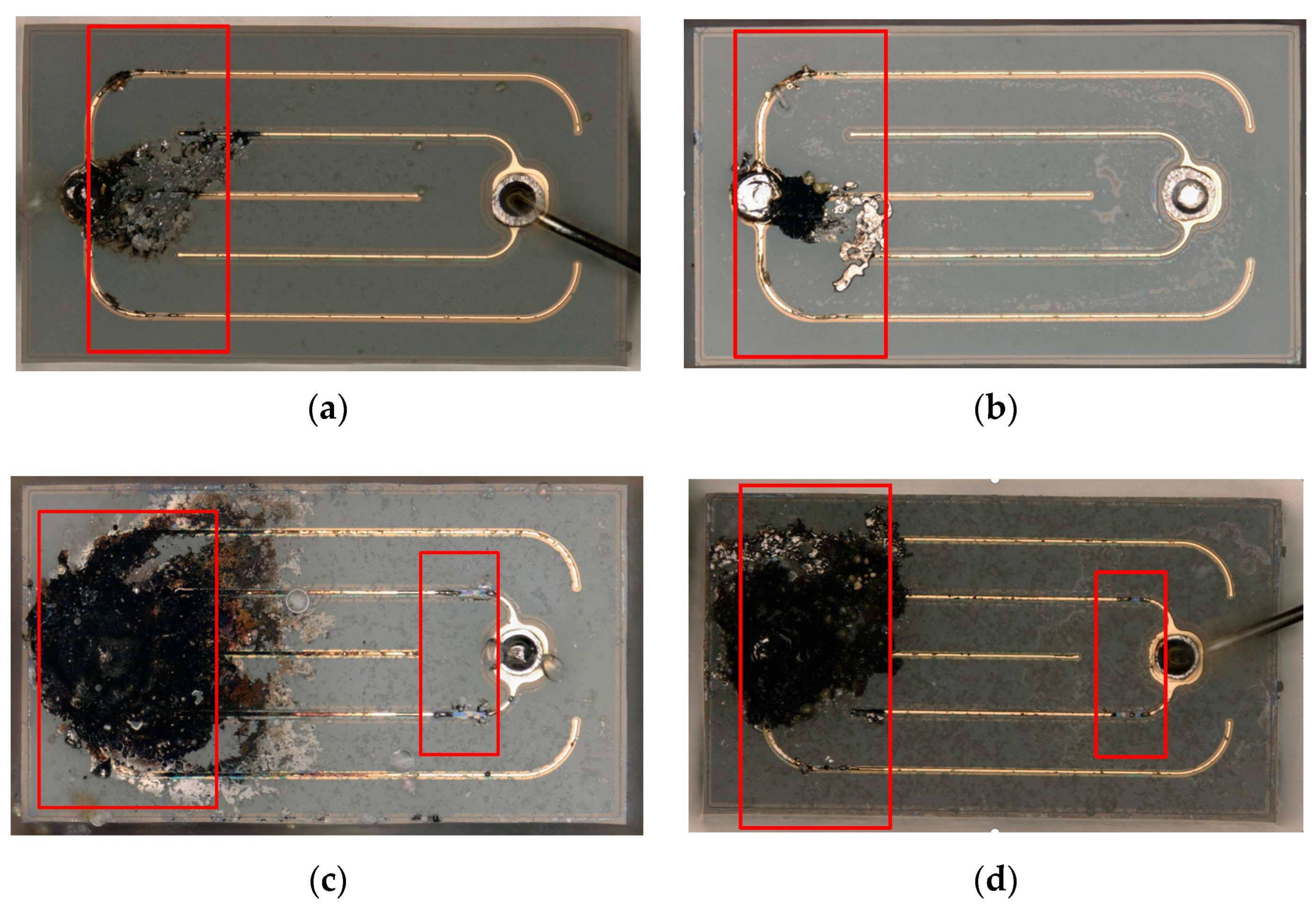
Figure 2.
Physical photo of LED failure microscope under different stresses. The red box indicates the location of the LED damage.
Figure 1 shows the cracking of the colloid in the middle of LEDs. The reason is that the stress of the colloid is released after the LED chip is burned, forming cracks.
2.2.2. Experiment Setting and Procedure
- Experiment setting
Specifications of the LED under test are shown in Table 1. The LED’s load current is 10 mA and can withstand a maximum current of 100 mA. The maximum test current selected in this article is 525 mA, but this current does not change the failure mechanism of the LEDs. In order to reduce the impact of changes in the LED manufacturing process or differences in material quality on this experiment, this paper selected products of the same batch of LEDs. The LOP was measured 8 times, and the average value was taken.

Table 1.
Specifications of the LED under test.
- 2.
- Number of testing samples
The normal operating temperature of the LEDs is 25 °C, the humidity is 40%, and the current is 10 mA, which is the standard normal vector of this experiment. Considering one failure in testing, the confidence level is 0.8, and the sample reliability is 95%. Then, the number of samples n should be greater than or equal to 59 for each experiment [14]. That is, the ideal confidence level can be achieved by selecting 59 samples for each of the five different stress combinations in this paper. The PCB board used in the test is a group of 10 LEDs. In this paper, 60 samples are selected for each group of stress testing.
2.2.3. Testing Profile
To improve the time-consuming acceleration time, the minimum temperature, humidity, and current in this paper are set to 85 °C, RH45%, and 20 mA, respectively. According to TM-28-14 [32], the minimum temperature is controlled at a higher 85 °C because the life of LEDs below 85 °C may exceed 10,000 h, which increases too much experimental time and cost. The normal operating humidity of the LEDs is 40%, and ADT requires that the minimum test humidity should be close to the maximum normal operating humidity. That is, this article chooses the humidity to be 45%. The minimum current is twice the rated current to accelerate the degradation time so that the degradation time does not exceed 10,000 h to reduce the time consumption. Yang et al. conducted a temperature accelerated life test on LED modules with an aging time of 1000 h, and the accelerated temperatures were 110 °C, 140 °C, and 170 °C [33]. Since current stress was added to the high-temperature experiment, 150 °C was selected as the highest temperature in this paper. In terms of current selection, we selected 150 °C, 400 mA, and 125 °C, 600 mA for testing. We found that the LED was damaged after 168 h at 150 °C and 400 mA, as shown in Figure 2a, and after 408 h at 125 °C, 600 mA, as shown in Figure 2b, which is inconsistent with the actual working condition of the LEDs. Under actual working conditions, the chip P-type electrode and P-finger burned, and the N-finger burned abnormally, as shown in Figure 2c. The chips under the above two working conditions all had P-type electrodes and P-fingers burned, and the N-finger had no obvious abnormality. However, under the two stress conditions of S4 and S5, the LEDs burned in accordance with the actual working conditions. Figure 2d below shows the 360 h LED failure under S4 stress, and both had P-type electrodes and P-fingers burned, and the N-finger burned abnormally.
The three stressors have been divided into 2, 3, and 4 levels, respectively. In particular, to better reflect the coupling effect of current and other stresses, this paper selects 20 mA, 220 mA, 300 mA, and 525 mA as four levels of current stress. Five different 3-stress test combinations are shown in Table 2 below.
Table 2.
Test conditions.
2.2.4. ADT Process
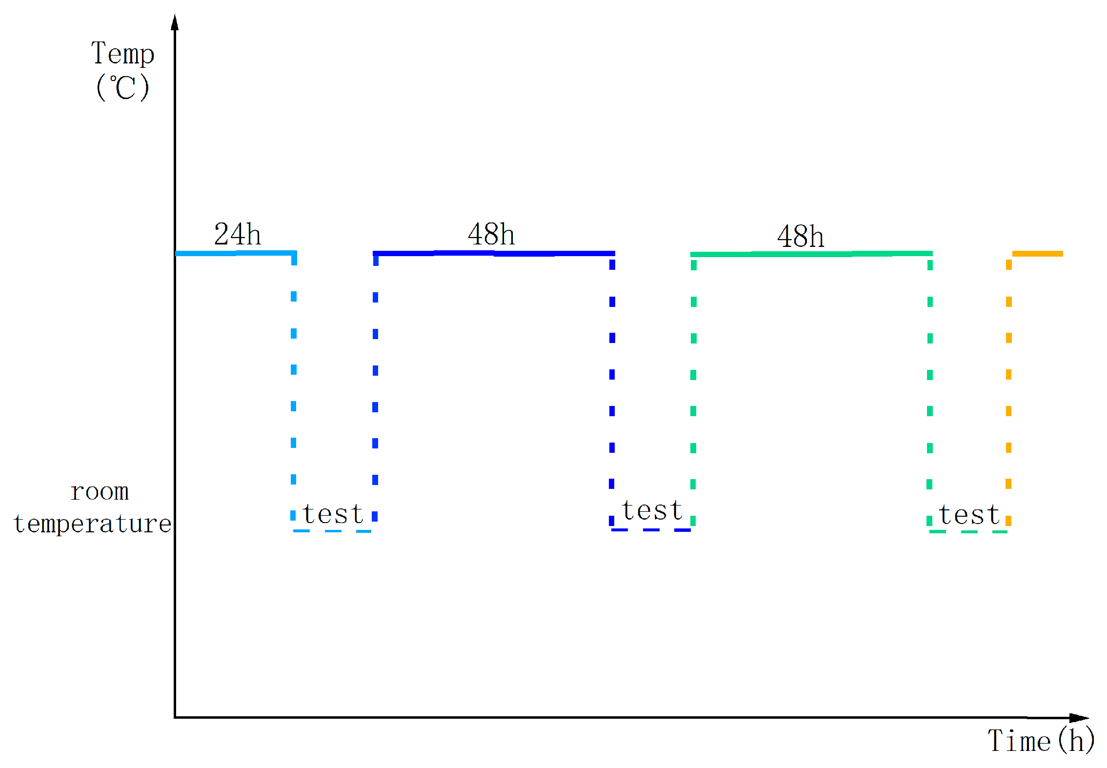
In the pre-experiment stage, the initial LOP value of each LED is first obtained. One experiment cycle has 4 or 5 steps, as shown below in Figure 3:
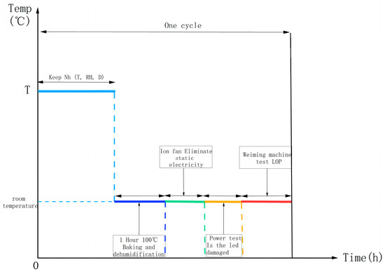
Figure 3.
Overview of a testing cycle.
- Put 6 groups of 10 LEDs into a PCB board under a certain condition for n hours;
- If the humidity of this experiment is 85%, it is necessary to bake and dehumidify for 1 h to prevent the PCB board from condensing with air and causing unexpected failure of the LED;
- Use an ion fan to remove static electricity to prevent the LED from being broken down when powered on;
- Use a power supply to test whether the LED is damaged;
- Put it into the Weimin tester to test the LOP of the LED.
To make the results more accurate and avoid the error caused by the extrapolation of the life test, this paper adopts a full-sample experiment and stops the experiment when all devices fail in 5 groups of 300 data. The specific process is shown in Figure 4 below. After completing the test under 5 pressures, the above 4 or 5 steps are carried out to obtain the LOP change after degradation for n hours.
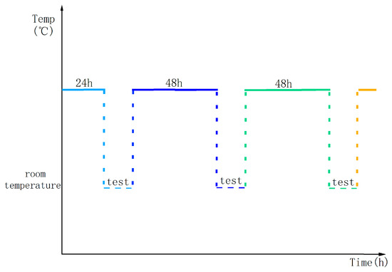
Figure 4.
ADT profile.
According to experience, under S1 conditions, the experimental time increases to about 1000 h after exceeding 1000. When the LOP BE decays close to the critical value of 30%, to make the failure time more accurate, it is necessary to record the LED position and perform an LOP BE test every 24 h to find its failure time. The test process is shown in Figure 4 below.
The x-axis in Figure 4 represents the degradation and test duration, the degradation duration is the first step in Figure 3, and the test time is steps 2–5 in Figure 3. The degradation time is different under different stresses, and the specific degradation time is the x-axis time in Figure 5. The test time under different stresses is also different. Since S2 and S3 have 85% humidity degradation, the test will go through step 2 in Figure 3, and the test time is longer than the remaining three groups of tests.
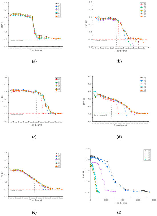
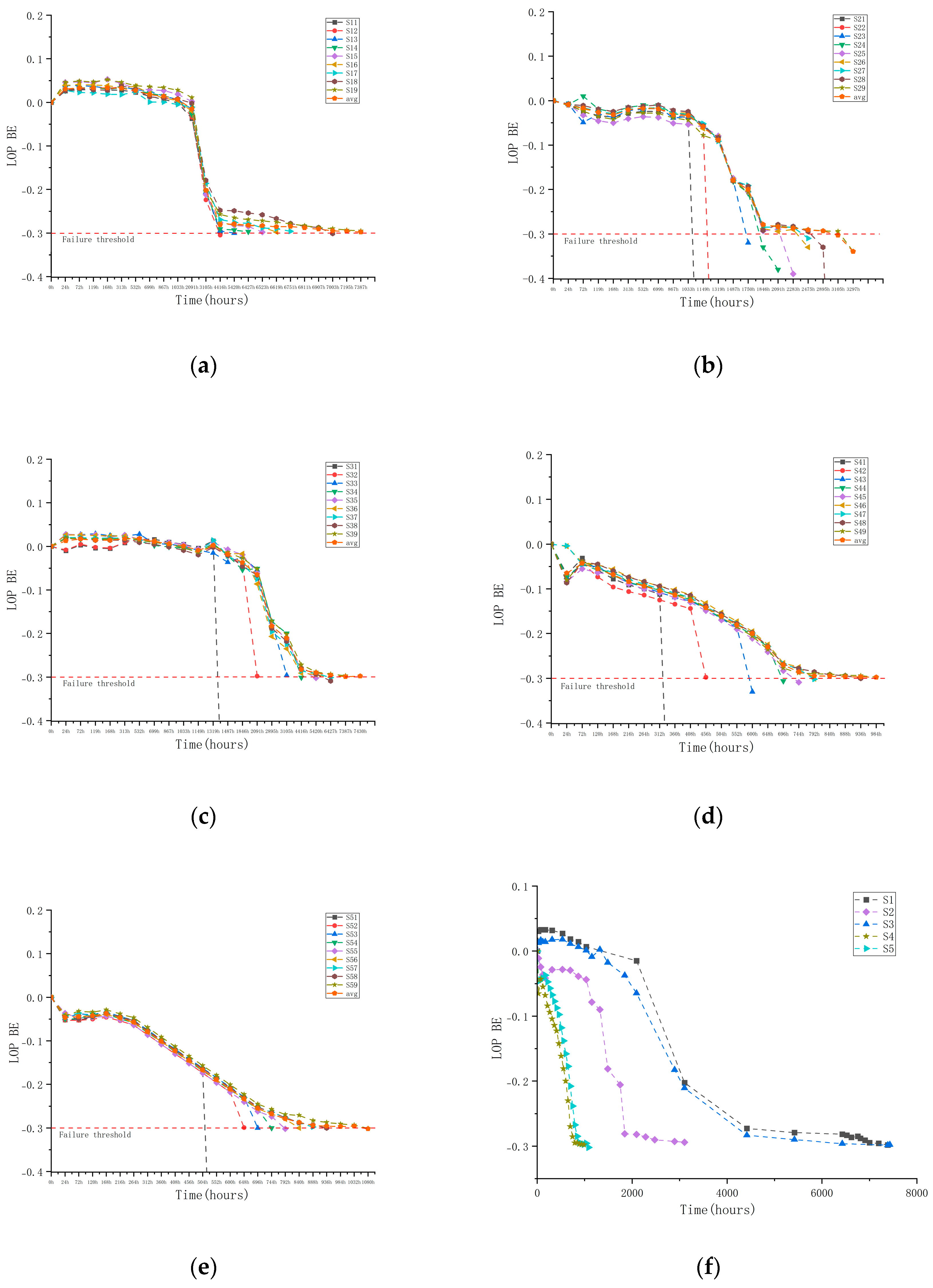
Figure 5.
LOP degradation curves of LEDs under 5 different stresses.
3. Results
The degradation paths of LEDs under S1-S5 stress are shown in the Figure 5 above. To avoid a cluttered image, only 9 LED degradations and the average degradation path of 1 LED path are shown under each stress, as shown in Figure 5 above. Figure 5f shows the average degradation path of 300 LEDs under S1–S5 stress.
Among them, S42 represents the second test sample under S4 stress. The tenth datum in each figure in Figure 5 is the average of the LOP BE of 60 data. Take Figure 5a as an example. When the initial situation is, according to the BE formula, the initial LOP BE is 0, and the x-axis is the measurement time of the LOP BE. The measurement time interval under different pressures is also different. It should be noted that the time line of the x-axis in Figure 5a–e is not proportional but only represents the measurement time. For example, the x-axis distance of 0–24 h is the same as 2091–3105 h, but the actual measurement time difference is very large. However, the x-axis in Figure 5f is proportional to time. Due to the relationship of retaining two decimal places, according to rounding, when the LOP BE value of the tested LEDs is −0.295 to −0.305, the LED is declared to be failed. The time recorded at this time is the LED failure time. When all 300 LEDs fail, the test is declared to be over. We can clearly see that the degradation is relatively mild under S1 stress, and the degradation of LEDs under S2 and S3 stresses will accelerate when the humidity and current are increased. Comparing the degradation of LEDs under S4 and S5 stresses, we can find that temperature is still the main stress that causes LED degradation, and the degradation of LEDs under S4 stress is also the fastest, followed by the degradation of LEDs under S5 stress. Through Figure 5f, we can clearly see the average degradation curve of 60 LEDs from S1 to S5, where the x-axis of each point is the average degradation time of the 60 LEDs, and the y-axis is the average LOP BE.
Under S1 stress, we found that the LOP change of the LED in the first 2091 h was positive; that is, the brightness was higher than the initial value; the LOP change rate also increased from 24 h to 72 h of S4 stress and from 120 h to 168 h of S5 stress. This may be the initial stage of LED self-luminous attenuation; that is, in the early stage of LED use, it may experience a stage of slight increase in light intensity. This is because, during the “aging” process of the device, the junction temperature changes, and material properties gradually stabilize, resulting in a slight increase in luminous efficiency. However, this phenomenon does not exist in the high-humidity S2 and S3 stresses, which may be due to the influence of high humidity on the initial growth of LOP. The Pearson Correlation Coefficient of S1-S5 is shown in Figure 6 below.
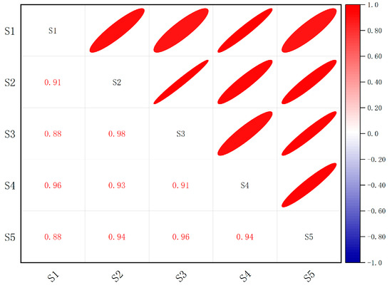
Figure 6.
S1–S5 Pearson Correlation Coefficient.
The Pearson Correlation Coefficient is an indicator used in statistics to measure the linear correlation between two variables. Its value is between −1 and 1. When the value is 1, it indicates a perfect positive correlation, which means that when one variable increases, the other variable will also increase linearly. When the value is −1, it indicates a perfect negative correlation, which means that when one variable increases, the other variable will decrease linearly. When the value is 0, it indicates no linear correlation, which means that there is no linear relationship between the two variables. In Figure 6, we can see that the Pearson Correlation Coefficient of S2 and S3 is 0.98. According to Table 2, the effect of current on the life of LEDs is strongly correlated; the Pearson Correlation Coefficient of S1 and S2 is 0.91, indicating that the effect of humidity and current on the life of LEDs is strongly correlated. The minimum value of the Pearson Correlation Coefficient between all stresses is 0.88, which also shows a high positive linear correlation. Therefore, the coupling relationship between the three stresses of temperature, humidity, and current must be considered.
4. Discussion
4.1. Statistical Data Analysis
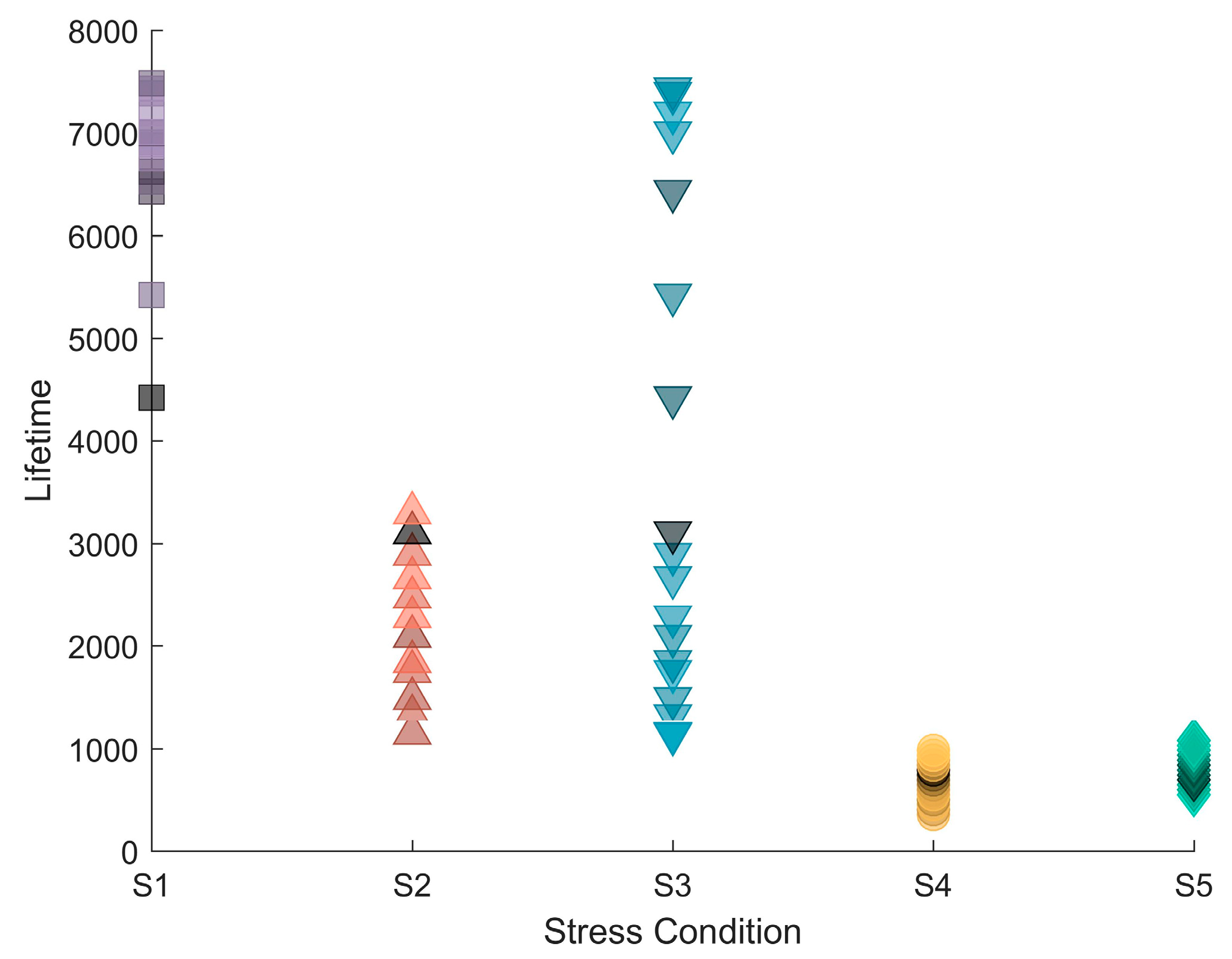
Figure 7 below is a scatter plot of the pseudo-life for LED. The darker the color, the more scatter plots there are for the same life. It can be seen from the Figure 7 below that the effect of increasing the current on the life of LED under S2 and S3 stress in humidity is not negligible. Obviously, the LED of S1 with temperature stress has the longest life, and the influence of temperature is greater than the influence of current increase; that is, the average life of LED under S4 stress is less than that under S5 stress.
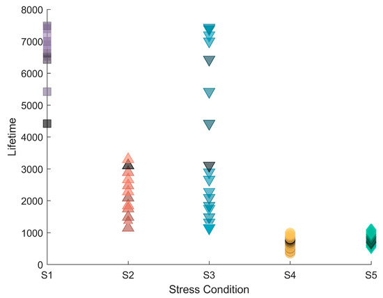
Figure 7.
Scatter plot of a pseudo-life for LED.
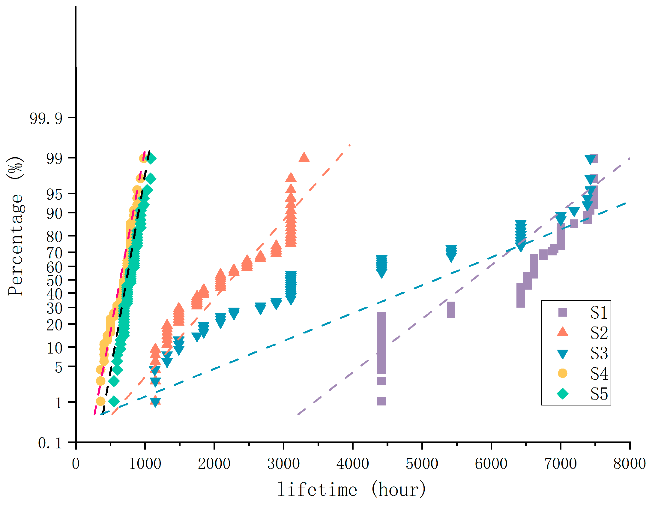
According to the S1–S5 life data obtained in Figure 7, we need to determine whether it meets Assumption 1, that is, whether the data conform to the Weibull distribution. This paper uses the Blom scoring method to find that the data best fit the Weibull distribution, and the Weibull distribution fit is as follows in Figure 8, where the x-axis represents the failure time under stress and the y-axis represents the percentile. The straight line running through the data is the ideal reference line obtained by theoretical calculation of the Weibull distribution, and its slope and intercept are related to the shape parameter and scale parameter of the Weibull distribution.
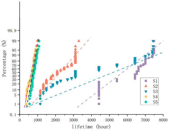
Figure 8.
S1–S5 Weibull distribution goodness of fit.
4.2. Modeling of Generalized Coupled Acceleration Model
Under high-temperature and high-humidity environments, metals and certain organic materials are prone to corrosion, resulting in the degradation of the performance of electrical connection components and packaging materials and increasing the risk of moisture penetration into LED packaging materials, which may cause physical and chemical changes in the materials, such as discoloration, softening, or deterioration. Therefore, it is believed that there is a coupling relationship between temperature and humidity; high temperature will accelerate the aging process of LED materials, especially organic materials (such as packaging resins) and certain semiconductor materials (such as chips and connecting wires) may fail or deteriorate due to high temperature. High current will cause increased heat inside the LED device, which may exceed the thermal capacity of the material and the processing capacity of the heat dissipation design, thereby affecting the stability and life of the material. Therefore, it is believed that there is a coupling relationship between temperature and current; in a high-humidity environment, water vapor can easily penetrate into the LED packaging material, causing the mechanical properties of the material to deteriorate, such as yellowing and cracking. Under high current, the heat generated by the LEDs increases, which will further aggravate the degradation of the material. This coupling of environment and electrical stress will accelerate the degradation process of the LEDs and shorten their life. Humidity will affect the interface between the LED chip and the package, which may cause current leakage, short circuit, and other problems. Under high current conditions, the interface problem will be more serious, which will lead to the degradation of the electrical performance of the LEDs, such as reduced luminous efficiency and color temperature drift. The combined effect of high humidity and high current will enhance the electromigration effect; that is, the metal atoms in the metal wire migrate under the action of the electric field, resulting in the breakage of the wire or increased resistance. This phenomenon is particularly significant under high current density and may eventually lead to the failure of the LEDs. Under the coupling of humidity and current, the failure mode of the LEDs may be more complex and difficult to predict. In this case, the reliability test results of the LEDs may be worse than under a single stress condition, and the failure rate in actual application will also be higher. In this experiment, increasing the current stress under humid conditions will reduce life, so it is believed that there is a coupling relationship between humidity and current. That is, this experiment has coupling terms of temperature and humidity, temperature and current, and humidity and current with three stresses. According to the acceleration model, the three-stress acceleration models without considering coupling, without considering wet–electric coupling, and considering the actual situation are as follows in Equation (15):
Among them, , , and represent the life of LEDs without considering stress coupling, without considering humidity–current coupling, and full coupling, respectively, represents the value to be estimated, a is 1–3, representing the above three cases, respectively, and b is the serial number of the value to be estimated.
4.3. Multi-Parameter Estimation Based on Particle Swarm Optimization
Equation (13) establishes the maximum likelihood function model of the multi-stress acceleration model. Since the multi-stress acceleration model has multiple parameters, there are nine parameters when the three stresses are coupled. The traditional Newton iteration method requires the gradient and Hessian matrix of Equation (13) and needs to provide the initial parameter estimation value, which has the disadvantages of a large amount of calculation and poor solution accuracy. The least squares method also needs to provide the initial parameter estimation value when fitting the nonlinear model of Equation (13), and the selection of the initial value has a significant impact on the optimal solution of the two models. This paper introduces the particle swarm algorithm to transform the parameter estimation problem into the optimal solution problem corresponding to the maximum likelihood function.
Particle Swarm Optimization (PSO) is a swarm intelligence optimization algorithm inspired by the collective behavior of biological groups such as bird flocks or fish schools. It was proposed by Kennedy and Eberhart in 1995 and was originally used to solve optimization problems. Later, it was widely used in various fields, such as engineering optimization, machine learning, and data mining. The algorithm has the characteristics of a simple and flexible algorithm structure, good globality, and fast convergence speed. It is suitable for continuous function extreme value problems and has strong global search capabilities for nonlinear and multi-peak problems.
First, define the variables in the particle swarm. In the multi-parameter optimization of the multi-stress acceleration model, the objective function value is the likelihood function, and the optimization goal is to find the maximum likelihood function. The distribution of the parameters is (lnα0, −α1, −α2, −α3, −α4, −α5, −α6, −α7, −β), which can be abbreviated as (a, b, c, d, e, f, g, h, β), where β is the shape parameter of the Weibull distribution. The process of particle swarm optimization is as follows:
- The positions and velocities of all particles are randomly initialized in the constraint space of the variables, ensuring that the constraint shape parameter β > 0 to ensure that the characteristic life is greater than 0;
- Calculate the objective function value of each particle, that is, the log-likelihood value of the test data under all stress combinations;
- For each particle, its current objective function value is compared with the optimal objective function value (pbest) in the particle’s history and the larger value of the two is selected and redefined as pbest;
- For each particle, its current objective function value is compared with the historical optimal objective function value (gbest) searched by all particles, and the larger value of the two is selected and redefined as gbest;
- Calculate the iteration speed and iteration position of each particle. The expressions are Equation (16).
Among them, are the speed and position of the particle at the k th iteration, independently generating two random numbers and between 0 and 1, and is the inertia coefficient representing the relative weight of the current speed. When running the initial iteration, a larger w value is selected to avoid falling into a local optimal solution due to a small step size. In the later stage of the iteration, the w value needs to be reduced to speed up the convergence and avoid curve oscillation. The expression of is set to , where is the maximum number of iterations set, and and are acceleration coefficients representing the relative weights of the historical optimal value of the particle and the historical optimal value of all particles. In the algorithm in this section, after comprehensive consideration of convergence accuracy and convergence speed, and are both taken as 2.05.
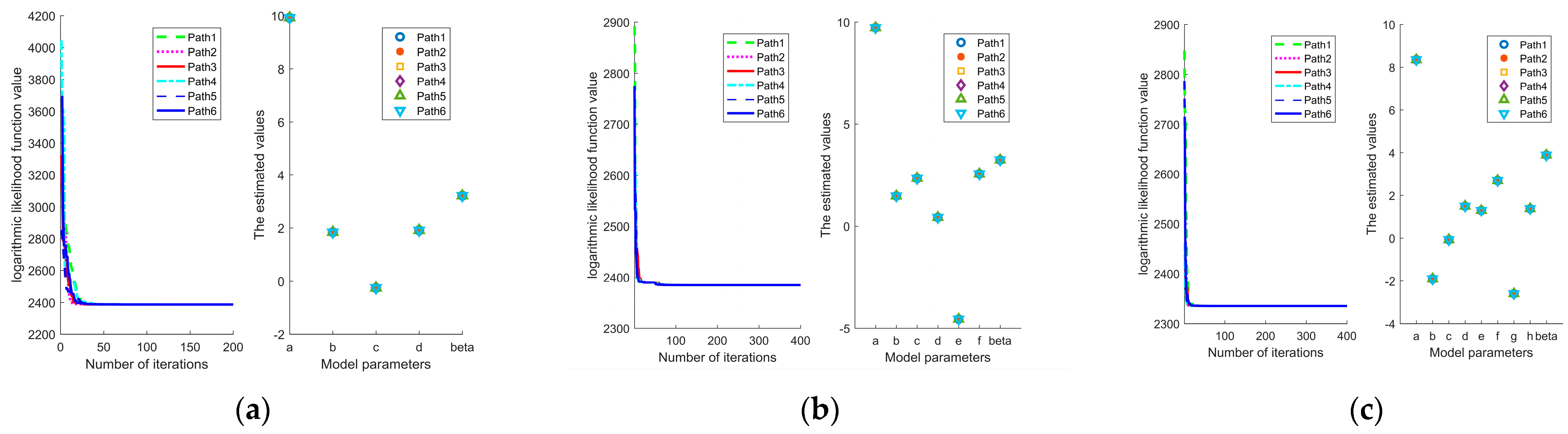
To ensure the accuracy of the parameters, the system randomly generates six different paths to calculate the target and takes the average of the estimated values of these six paths as the estimated parameters. When coupling is not considered, 100 particles are taken, the dimension is 5, the maximum number of iterations is 200, and the parameter vectors estimated by the six different paths are shown in Figure 9a below. When humidity–current coupling is not considered, 100 particles are taken, the dimension is 7, the maximum number of iterations is 400, and the parameter vectors estimated by the six different paths are shown in Figure 9b below. When full coupling is taken, 100 particles are taken, the dimension is 9, the maximum number of iterations is 400, and the parameter vectors estimated by the six different paths are shown in Figure 9c below. The parameter estimates of the three different models in Equation (15) are shown in Table 3.
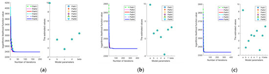
Figure 9.
Parameter estimation for three models. (a): 3-stress coupling is not considered; (b): wet electrical coupling is not considered; (c): fully coupled.
Table 3.
Three-stress parameter estimates of Weibull distribution.
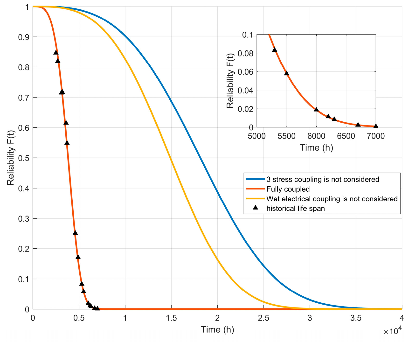
Finally, the life index under normal stress levels (25 °C, 40%RH, 10 mA) can be extrapolated through the solved multi-stress coupling model. The life estimation results of the full coupling model, the particle swarm algorithm without considering humidity–current coupling, and the coupling model are given and compared with the historical life in reliability prediction. The results are shown in Figure 10 below.
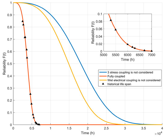
Figure 10.
Evaluation results of different models under normal stress.
According to the blue line in Figure 10, the average life of LEDs is 20,330 h without considering stress coupling, which meets the manufacturer’s standard of 20,000 h for LEDs. However, the actual life is worrying. Without considering the coupling of humidity and current, the life is also very different from the actual situation. It is also problematic to have the life too close to the actual life when considering full coupling because the failure of LEDs includes many aspects, including occasional failure and degradation failure. The historical life scatter points include more stress combinations, such as the number of switching LEDs, salt spray, alternating hot and cold in the morning and evening, and other external factors, as well as different LED manufacturing processes, differences in material quality, and other internal factors, which will lead to the diversity of LED life. There are also defects in the design of the experiment, such as not considering the impact of high temperature and self-heating on humidity, whether the constant temperature, humidity, and current experiment can replace the degradation of LEDs in the real environment, etc. However, it is undeniable that it is still not in line with the actual situation without considering stress coupling. It can be concluded that the full coupling between the three stresses has a great impact on the accuracy of the product life estimation, and the full coupling effect must be considered in LED life assessment.
5. Conclusions
Given the complex environment in which LEDs operate, this paper first proposes a multi-stress accelerated degradation evaluation method considering generalized coupling based on the traditional Arenas model. Secondly, a new gradient three-stress accelerated degradation experiment is designed to find out the coupling relationship between current, temperature, and humidity. Then, for the accuracy of the data, the life extrapolation method is not used. A multi-stress generalized coupling parameter MLE method for the entire sample is proposed, and the particle swarm algorithm is used to obtain unknown parameters to solve the multi-parameter estimation problem of the multi-stress accelerated model. Finally, it is verified that current coupling is not negligible in this LED, and the maximum error with the historical life scatter points is 6.5%, which can effectively solve the problem of poor accuracy in LED life prediction.
This paper only considers one degradation failure of three-stress coupling, which is still different from the actual working conditions and has some limitations. Considering only the three stresses on LEDs as a benchmark is obviously not comprehensive enough and does not fully address potential confounding factors that may affect the reliability of the results, such as variations in LED manufacturing processes or differences in material quality, changes in humidity levels under high-temperature environments and self-heating conditions, etc. Further research and discussion are needed in tests of more stress coupling environments, such as low temperature, vibration and salt spray, and competition failure between degradation failure and accidental failure. In addition, the failure analysis of different LED materials and structures in multi-stress coupling environments is also a future development direction.
Author Contributions
Conceptualization, Z.Z. and Y.D.; methodology, Z.Z., Y.D., and K.L.; software, Y.D.; validation, Y.D. and K.L.; investigation, Z.Z. and X.Y.; writing—original draft preparation, Y.D.; writing—review and editing, Y.D. and X.Y. All authors have read and agreed to the published version of the manuscript.
Funding
This research received no external funding.
Institutional Review Board Statement
Not applicable.
Informed Consent Statement
Not applicable.
Data Availability Statement
The data that support the findings of this study are available from the author (Y.D.) upon reasonable request.
Acknowledgments
Thanks to all of the authors cited in this article and the referees for their helpful comments and suggestions.
Conflicts of Interest
The authors declare no conflicts of interest.
Appendix A
Based on the relationship in the Arrhenius model that the life is proportional to the reverse reaction rate, the relationship between the life and stress under the combined action of the corresponding N stress satisfies the following Equation (A1):
Taking the logarithm of both sides gives the following Equation (A2):
Stress normalization of the above formula yields the following Equation (A3):
Combined with Equation (7), the multi-stress acceleration model in which the characteristic life follows the Weibull distribution can be obtained as follows Equation (A4):
In particular, the multi-stress acceleration model under the combined action of three stresses, where the life obeys the Weibull distribution, is Equation (A5):
References
- Chang, M.-H.; Das, D.; Varde, P. Light emitting diodes reliability review. Microelectron. Reliab. 2012, 52, 762–782. [Google Scholar] [CrossRef]
- Meneghini, M.; Podda, S.; Morelli, A.; Pintus, R.; Trevisanello, L.; Meneghesso, G. High brightness GaN LEDs degradation during DC and pulsed stress. Microelectron. Reliab. 2006, 46, 1720–1724. [Google Scholar] [CrossRef]
- Tan, C.M.; Chen, B.K.E.; Xu, G.; Liu, Y. Analysis of humidity effects on the degradation of high-power white LEDs. Microelectron. Reliab. 2009, 49, 1226–1230. [Google Scholar] [CrossRef]
- Trevisanello, L.; Zuani, F.D.; Meneghini, M.; Trivellin, N.; Zanoni, E.; Meneghesso, G. Thermally activated degradation and package instabilities of low flux LEDs. In Proceedings of the 2009 IEEE International Reliability Physics Symposium, Montreal, QC, Canada, 26–30 April 2009; pp. 98–103. [Google Scholar]
- Mehr, M.Y.; Van Driel, W.D.; Zhang, G.Q. Reliability and lifetime prediction of remote phosphor plates in solid-state lighting applications using accelerated degradation testing. Electron. Mater. 2016, 45, 444–452. [Google Scholar] [CrossRef]
- Nogueira, E.; Orlando, V. Accelerated life test of high luminosity blue LEDs. Microelectron. Reliab. 2016, 64, 631–634. [Google Scholar] [CrossRef]
- Li, Y.; Pan, G.Z. A novel accelerated life-test method under thermal cyclic loadings for electronic devices considering multiple failure mechanisms. Microelectron. Reliab. 2020, 144, 11–17. [Google Scholar] [CrossRef]
- Yang, Z.; Chen, Y. Smart electricity meter reliability prediction based on accelerated degradation testing and modeling. Int. J. Electr. Power Energy Syst. 2014, 56, 209–219. [Google Scholar] [CrossRef]
- Lin, K.; Chen, Y. Reliability assessment model considering heterogeneous population in a multiple stresses accelerated test. Reliab. Eng. Syst. Saf. 2017, 165, 134–143. [Google Scholar] [CrossRef]
- Wang, Y.; Chen, X. Optimal design of step-stress accelerated degradation test with multiple stresses and multiple degradation measures. Qual. Reliab. 2017, 33, 1655–1668. [Google Scholar] [CrossRef]
- Miao, H.; Guo, W. Lifetime prediction of UV LEDs based on Bayesian MCMC and other models. Acta Opt. Sin. 2024, 44, 2223001. [Google Scholar]
- Liang, B.; Wang, Z.; Qian, C. Investigation of step-stress accelerated degradation test strategy for ultraviolet light emitting diodes. Materials 2019, 12, 3319. [Google Scholar] [CrossRef] [PubMed]
- Ibrahim, M.S.; Jing, Z.; Yung, W.K.C. Bayesian based lifetime prediction for high-power white LEDs. Expert Syst. Appl. 2021, 185, 115627. [Google Scholar] [CrossRef]
- Liu, Y.; Wang, Y. A new universal multi-stress acceleration model and multi-parameter estimation method based on particle swarm optimization. Proc. Inst. Mech. Eng. Part O J. Risk Reliab. 2020, 234, 764–778. [Google Scholar] [CrossRef]
- Zhang, F.; Tian, R. Multi-stress accelerated life evaluation method considering generalized coupling. J. Syst. Eng. Electron. 2023, 45, 3350–3361. [Google Scholar]
- Escobar, L.A.; Meeker, W.Q. A review of accelerated test models. IMS 2006, 21, 552–577. [Google Scholar] [CrossRef]
- Wang, M.; Wang, S. Reliability analysis of ball screw based on double-stress accelerated life testing. J. Beijing Univ. Chem. Technol. 2022, 48, 703–709. [Google Scholar]
- Kang, Q.; Li, Y. Reliability estimation of thin film platinum resistance MEMS thermal mass flowmeter by step-stress accelerated life testing. Microelectron. Reliab. 2023, 147, 115026. [Google Scholar] [CrossRef]
- Amleh, M.A.; Raqab, M.Z. Inference in simple step-stress accelerated life tests for Type-II censoring Lomax data. JSTA 2021, 20, 364–379. [Google Scholar] [CrossRef]
- Abd El-Raheem, M.A.M.; Abu-Moussa, M.H. Accelerated Life Tests under Pareto-IV Lifetime Distribution: Real Data Application and Simulation Study. Mathematics 2020, 8, 1786. [Google Scholar] [CrossRef]
- Indmeskine, F.E.; Saintis, L.; Kobi, A. Review on accelerated life testing plan to develop predictive reliability models for electronic components based on design-of-experiments. Qual. Reliab. 2023, 39, 2594–2607. [Google Scholar] [CrossRef]
- Wang, H.; Teng, K. Design an optimal accelerated-stress reliability acceptance test plan based on acceleration factor. IEEE Trans. Reliab. 2018, 67, 1008–1018. [Google Scholar] [CrossRef]
- Nassar, M.; Dobbah, S.A. Inference on Constant Stress Accelerated Life Tests Under Exponentiated Exponential Distribution. EJASA 2023, 16, 234–256. [Google Scholar]
- Lee, I.C.; Hong, Y. Sequential Bayesian Design for Accelerated Life Tests. Technometrics 2018, 60, 472–483. [Google Scholar] [CrossRef]
- Alotaibi, R.; Almetwally, E.M. Optimal test plan of step stress partially accelerated life testing for alpha power inverse Weibull distribution under adaptive progressive hybrid censored data and different loss functions. Mathematics 2022, 10, 4652. [Google Scholar] [CrossRef]
- Wang, F.-K.; Chu, T.-P. Lifetime predictions of LED-based light bars by accelerated degradation test. Microelectron. Reliab. 2012, 52, 1332–1336. [Google Scholar] [CrossRef]
- Levada, S.; Meneghini, M.; Meneghesso, G. Analysis of dc current accelerated life tests of GaN LEDs using a weibull-based statistical model. IEEE Trans. Device Mater. Reliab. 2005, 5, 688–693. [Google Scholar] [CrossRef]
- Lu, G.; Yang, S.; Huang, Y. Analysis on failure modes and mechanisms of LED. In Proceedings of the 8th International Conference on Reliability, Maintainability and Safety, Chengdu, China, 20–24 July 2009; pp. 1237–1241. [Google Scholar]
- Meneghesso, G.; Levada, S.; Zanoni, E.; Podda, S.; Mura, G.; Vanzi, M.; Cavallini, A.; Castaldini, A.; Du, S.; Eliashevich, I. Failuremodes and mechanisms of DC-aged GaN LEDs. Phys. Status Solidi A 2002, 194, 389–392. [Google Scholar] [CrossRef]
- Khan, A.; Hwang, S.; Lowder, J. Reliability issues in AlGaN based deep ultravioletlight emitting diodes. In Proceedings of the IEEE 47th Annual International Reliability Physics Symposium, Montreal, QC, Canada, 26–30 April 2009; pp. 89–93. [Google Scholar]
- Zhang, J.-M.; Zou, D.-S.; Xu, C.; Zhu, Y.-X.; Liang, T.; Da, X.-L.; Shen, G.-D. High power and high reliability GaN/ InGaN flip-chip light-emitting diodes. Chin. Phys. 2007, 16, 1135–1139. [Google Scholar]
- IES TM-28-14; Projecting Long-Term Luminous Flux Maintenance of LED Lamps and Luminaires. IES-USA: New York, NY, USA, 2014.
- Yang, Y.-H.; Su, Y.-F.; Chiang, K.-N. Acceleration factor analysis of aging test on gallium nitride (GaN)-based high power light-emitting diode (LED). In Proceedings of the Intersociety Conference on Thermal and Thermomechanical Phenomena in Electronic Systems (ITherm), Orlando, FL, USA, 27–30 May 2014; pp. 178–181. [Google Scholar]


Disclaimer/Publisher’s Note: The statements, opinions and data contained in all publications are solely those of the individual author(s) and contributor(s) and not of MDPI and/or the editor(s). MDPI and/or the editor(s) disclaim responsibility for any injury to people or property resulting from any ideas, methods, instructions or products referred to in the content. |
© 2024 by the authors. Licensee MDPI, Basel, Switzerland. This article is an open access article distributed under the terms and conditions of the Creative Commons Attribution (CC BY) license (https://creativecommons.org/licenses/by/4.0/).