Characterization of Seismic Signal Patterns and Dynamic Pore Pressure Fluctuations Due to Wave-Induced Erosion on Non-Cohesive Slopes

Abstract

Wave erosion of slopes can easily trigger landslides into marine environments and pose severe threats to both the ecological environment and human activities. Therefore, near-shore slope monitoring becomes crucial for preventing and alerting people to these potential disasters. To achieve a comprehensive understanding, it is imperative to conduct a detailed investigation into the dynamics of wave erosion processes acting on slopes. This research is conducted through flume tests, using a wave maker to create waves of various heights and frequencies to erode the slope models. During the tests, seismic signals, acoustic signals, and pore pressure generated by wave erosion and slope failure are recorded. Seismic and acoustic signals are analyzed, and time-frequency spectra are calculated using the Hilbert–Huang Transform to identify the erosion events and signal frequency ranges. Arias Intensity is used to assess seismic energy and explore the relationship between the amount of erosion and energy. The results show that wave height has a more decisive influence on erosion behavior and retreat than wave frequency. Rapid drawdown may potentially cause the slope to slide during cyclic swash and backwash wave action. As wave erosion changes from swash to impact, there is a significant increase in the spectral magnitude and Power Spectral Density (PSD) of both seismic and acoustic signals. An increase in pore pressure is observed due to the rise in the run-up height of waves. The amplitude of pore pressure will increase as the slope undergoes further erosion. Understanding the results of this study can aid in predicting erosion and in planning effective management strategies for slopes subject to wave action.

1. Introduction

Coastal slopes are often subject to wave erosion, leading to landslides into marine environments. Wave erosion not only exposes the slope and causes soil loss but also severely threatens the ecology, human activities, and the safety of public facilities. A “marine geohazard” is defined as geological features and processes in coastal and offshore environments that lead to loss of life and assets [1,2,3,4,5,6]. The fundamental problems of marine geohazards are highlighted, such as coastal erosion, beach erosion, and retreat, among others. To develop corresponding mitigation measures, it is crucial to monitor and investigate the failure mechanisms of slopes under wave erosion.

The investigation into geomorphological changes in slope profiles caused by wave erosion has been a focus of numerous studies, each contributing to our understanding of coastal dynamics, erosion processes, and the mechanisms behind bluff and cliff retreat. Vallejo [7] examined how unconsolidated coastal bluffs along the Great Lakes in the USA respond to wave action, uncovering patterns of bluff retreat and incorporating these findings into slope evolution models. These models provide insights into recession rates and the impact of wave action on bluff stability. Similarly, Shipman [8] focused on coastal bluffs and sea cliffs on Puget Sound, Washington, USA, identifying wave action as a key driver of erosion. Shipman’s work highlighted the vulnerability of sedimentary layers to erosion and the importance of beach and berm geometry in protecting bluffs from wave-induced erosion in shielding the bluff toe from direct wave contact. Hampton et al. [9] provided comprehensive overviews of coastal cliff formation, evolution, stability, and the dual influence of terrestrial processes and wave action. They noted the episodic nature of wave impact and cliff retreat, influenced by the wave climate, and identified wave action at the base of landslides and high groundwater levels as key triggers for large coastal landslides. Kawamura and Miura [10] and Ji et al. [11] contributed to understanding the mechanisms behind wave-induced erosion and its impact on coastal geology. Kawamura and Miura’s physical model tests shed light on the failure mechanism of coastal cliffs, while Ji et al. [11] explored the geomorphic evolution of reservoir banks due to wave erosion, demonstrating the formation of a stepped topography influenced by wave actions. Qin et al. [12] and Ozeren et al. [13] investigated erosion processes in specific coastal environments, with Qin et al. focusing on riverside slope failure due to wind wave erosion and Ozeren et al. examining wave-impacted embankment slopes. Both studies emphasized the correlation between wave characteristics and the erosion process. Morales et al. [14] and Alberti et al. [15] studied the dynamics of coastal cliffs and platforms, noting the significant influence of wave processes on coastal morphology and the triggering of landslide activity by a combination of wave-induced erosion and substantial rainfall. These studies highlight the differential erosion along coastlines and the importance of geological and climatic factors in coastal stability and erosion rates.

The retreat of coastal slopes due to erosion is a critical concern for coastal management and environmental sustainability. Carpenter et al. [16] discussed the recession rates of soft cliffs. They indicated that the rate of sea level rise and strength of the costal materials control the cliff retreat and shore profile. Castedo et al. [17] investigated wave erosion on clay coasts. They concluded that bluff crest recession rates are highest during high water levels, and the bluff slopes failed in rotational slides and topples. The volume and morphology of the beach significantly influence the frequency and intensity of run-up reaching the bluff face, thus impacting the rates of bluff recession. Wang et al. [18] revealed that waves scour soil particles as they climb the slope, eventually leading to wave erosion niches and collapses. The erosion rate initially peaks then decays exponentially.

Many scholars have studied the characteristics of slope failure through seismic signals. Feng et al. [19] identified three types of riverbank landslides through model tests and found that the characteristics and processes of these landslides correspond to their seismic signals and time-frequency spectra. The three types of riverbank landslides are as follows. (a) Single landslide: Soil slides along the same sliding surface. (b) Intermittent landslide: Soil gradually slides intermittently along the same sliding surface. (c) Successive landslide: Different soils continuously slide from different sliding surfaces. Feng et al. [20] conducted model tests simulating landslides due to seepage and identified precursor signals from single landslide-induced seismic signals, which are helpful for landslide early warning. Feng et al. [21] recorded seismic signals of a slope model in a field test, showing that seismic signals of landslide events can be recognized even when the slope model is eroded by floods. Chang et al. [22] explained the main physical processes of rock slope failure through seismic signals. Their research showed that rock slope failure events mainly include multiple mass slides, toppling, and interactions of rock mass. Multiple rockslides present pulse-like characteristics in the time-frequency spectrum, reflecting the sudden, brief seismic peaks generated each time rocks hit the ground. Boulders impacting show columnar features in the time-frequency spectrum, indicating a period of intense vibration. Slope sliding and rock collisions produce different seismic time-frequency spectrum traces, which help to distinguish different landslide events. Helmstetter and Garambois [23] analyzed the seismic signals of rockfall events of different sizes. Their findings indicated that smaller rockfall events, involving less rock mass or covering smaller areas, produced seismic signals mainly concentrated at higher frequencies; larger rockfall events, involving more massive rocks or covering more extensive areas, produced stronger low-frequency responses. This demonstrates that different collapse behaviors produce distinct collapse intensities and delays. By monitoring seismic signals, we can track these events.

The impact of wave erosion on slope stability, particularly through changes in pore pressure, has been a significant focus of research across various studies. Zhao et al. [24] explored how water level changes and wave erosion affect slope stability, noting the roles of seepage, wave swash, and hydraulic gradient in reducing soil strength and potentially leading to slope failure. Hegge and Masselink [25] studied interactions between swash and groundwater, finding that swashes extending above the mean groundwater level cause a rise in the groundwater table, impacting slope stability. Peng et al. [26] used flume experiments to study the influence of water level and wave height on dam stability, demonstrating the relationship between pore pressure changes and wave activity.

Monitoring the acoustic signals of wave erosion and slope failure helps to understand the condition of wave-eroded slopes. Previous research has indicated that seismic signals associated with the movement of materials and acoustic signals are related and complementary. The combination of these two types of sensors can serve as the basis for disaster monitoring and warning systems. However, research on the analysis of acoustic signals from wave-eroded slopes is currently lacking, with most studies focusing on debris flows and rockfall events. Nevertheless, valuable insights and characteristics of acoustic signals can still be gleaned from these studies. Huang et al. [27] explored the differences between seismic and acoustic signals generated by rocks in riverbeds and indicated that the attenuation rate of acoustic signals in the air is much less than the attenuation rate of seismic signals on the ground. This suggests that acoustic signals can be captured at relatively greater distances, aiding in monitoring over broader areas. Moreover, the data showed that the frequency range of seismic and acoustic signals generated by rock impacts on riverbeds is roughly the same. This frequency similarity indicates that ground seismic signals and airborne acoustic signals originate from the same seismic source, which is crucial for analyzing and interpreting natural phenomena. Chou et al. [28] analyzed the acoustic signals generated by debris flows and found that sound signals can reflect the dynamic characteristics of debris flows. For example, the peak frequency of the signal is related to parameters such as the velocity, depth, and discharge of the debris flow. Liu et al. [29] studied the acoustic signals of debris flows using data from flume experiments and actual monitoring. The research revealed that in the absence of strong external interference, debris flow acoustic signals can be easily distinguished from environmental noise based on their characteristics. For instance, debris flow acoustic signals typically have a very long duration compared to the shorter duration of other noise sources. Acoustic signals, similar to seismic signals, can provide information about the characteristics of material movement and help identify different events through signal features such as duration, amplitude, and spectrum. In general, the breaking and splashing of waves produce sound, and the louder the impact of waves on slopes, the louder the sound may be. Friction between soil particles during slope movement also generates sound. Based on the fact that wave erosion and slope sliding produce acoustic signals with different characteristics, monitoring acoustic signals can help us indirectly infer the intensity of wave impacts or identify coastal slope failure events.

The purpose of this study is to investigate the dynamic characteristics of seismic signals, acoustic signals, and pore pressure of slopes under various wave erosion conditions. Therefore, we conducted multiple sets of flume tests involving wave erosion, using waves with varying heights and frequencies to erode the slope models. Seismic and acoustic signals were analyzed using the Hilbert–Huang transform. This study explains the variations in seismic and acoustic signals as well as pore pressure during the test process. We also analyzed the seismic signals generated during slope model sliding and collapses in the tests. Additionally, we conducted a parameter analysis to investigate the influence of wave height and frequency on slope erosion. We obtained some important findings. Wave height plays a more critical role in coastal erosion and retreat than wave frequency; the phenomenon of rapid drawdown, triggered by cyclical swash and backwash, is a key factor inducing slope slides; a shift in erosion mechanisms from swash to direct impact is noted to elevate seismic and acoustic signals, indicating a change in the erosion dynamics. Furthermore, an increase in wave run-up height leads to elevated pore pressure within slope, which is a precursor to intensified erosion. These insights underline the complex interplay between wave dynamics and coastal erosion processes, and can serve as a reference for the implementation of coastal slope monitoring and prewarning.

2. Methods

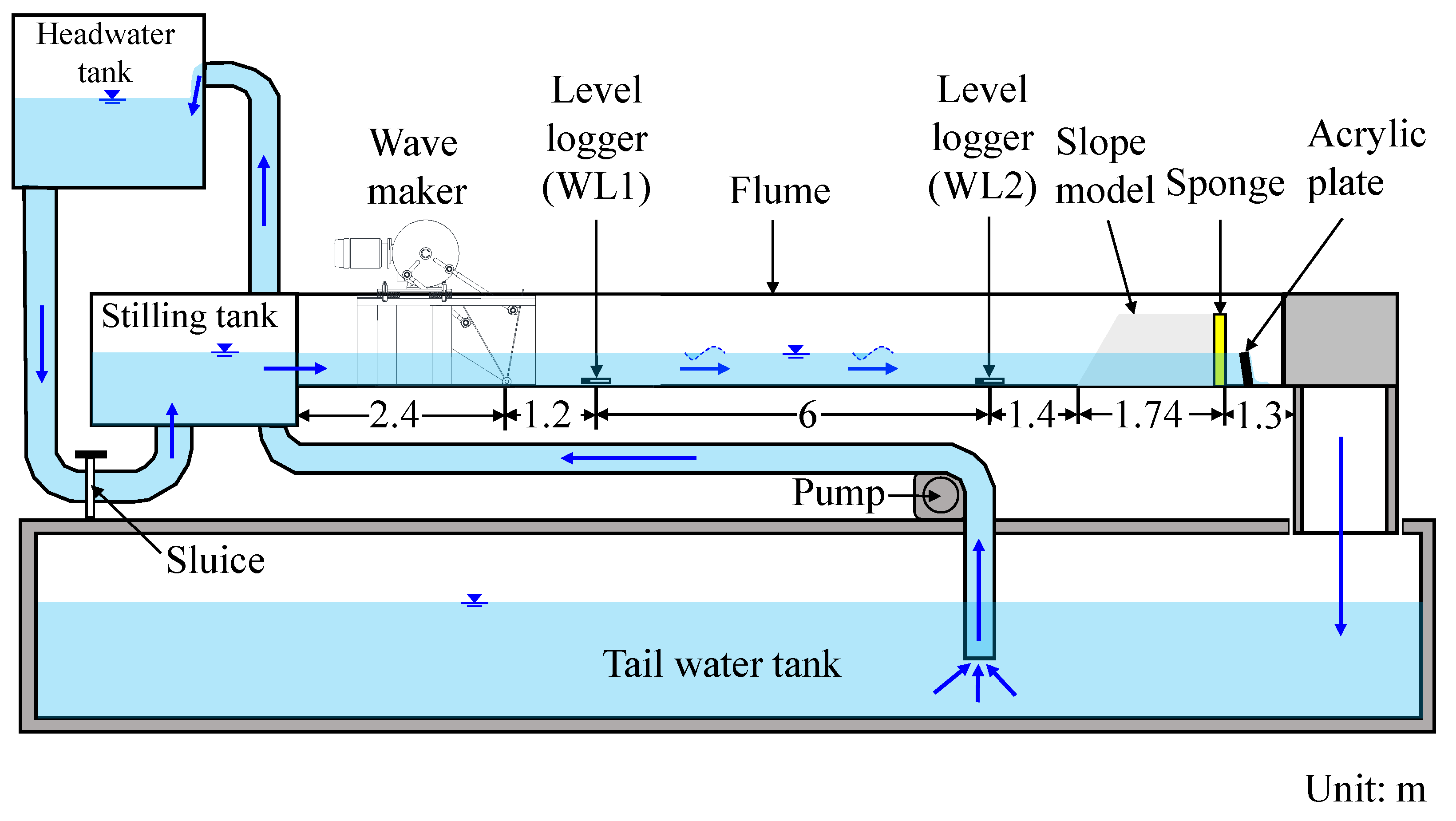
2.1. Flume Configuration

The test setup of Ozeren et al. [13] and Peng et al. [26] was referred to for this study. Within the flume, the wave maker and slope models were configured. The wave maker employed a flap-type design capable of generating waves with varying frequencies and wave heights. During the tests, water level changes were measured. We evenly poured sand into the slope model area in the flume and built it layer by layer without compaction, aiming to keep it loose and easily erodible for inducing damages. At the back of the slope model, a sponge and acrylic plate were installed. The sponge was fixed by a plate with drain space and served to prevent the loss of slope materials while directing water toward the acrylic plate behind it. The acrylic plate allowed water to overflow out of the flume so that the water level in the flume could be controlled. The flume used for the model tests measures 15 m × 0.6 m × 0.6 m (L × W × H), as shown in Figure 1. This flume is the same one used by Feng et al. [19]. The bottom of the flume has a slope of 0.1%. Water was pumped from a reservoir to the headwater. The water entering the water tank from the headwater is controlled by the sluice.

2.2. Slope Model and Layout of the Sensors

Table 1. The dimensions of the slope model.

Sloping of the Slope Model β [°]	Height of the Slope Model H [m]	Top Length of the Slope Model L1 [m]	Bottom Length of the Slope Model L2 [m]	Initial Water Level Hi [m]
40	0.6	1.1	1.7	0.3

lists the dimensional information of the slope model. We used uniform rounded sands to construct homogeneous non-cohesive slope models. The source of the sands is Vietnam. After the sieve analyses, the grain size parameters of the sands were obtained as D₅₀ = 1.74 mm, D₁₀ = 0.94 mm, and D₉₀ = 3 mm. The model’s average moist unit weight is approximately 1.447 t/m³, while the dry unit weight is about 1.429 t/m³. The water content by weight is measured at around 1.5%. To ensure that the slope materials are loose and easily damaged, we did not compact them during the model-building process. After the slope model was built, we let the model sit still for 5 h to allow moisture in the model to distribute naturally before conducting the tests.

The layout of sensors is as shown in Figure 2. This study used 3 accelerometers (Acc 1–3) and 4 pore pressure gauges (PP1–4) to record the seismic signals and pore pressure of the slope models. The wave level is measured by two wave gauges (WL1, WL2), positioned 7.4 and 1.4 m away from the toe of the slope model, as shown in Figure 1. We also placed a microphone (Mic) above the surface of the slope model to record the acoustic signals of slope erosion and slide/collapse caused by waves. The specifications of the accelerometers and the microphone are listed in Supplementary Tables S1 and S2. In addition, 3 cameras were set up during the tests to record the front, top, and side views of the slope model.

2.3. Data Analysis

To quantify the relationship between wave height, wave frequency, slope erosion, and slope retreat, we defined significant wave height (Holthuijsen [30]), erosion ratio, and retreat. The run-up height reflects the wave erosion range and influences pore pressure in the slope, so we also defined the wave run-up height.

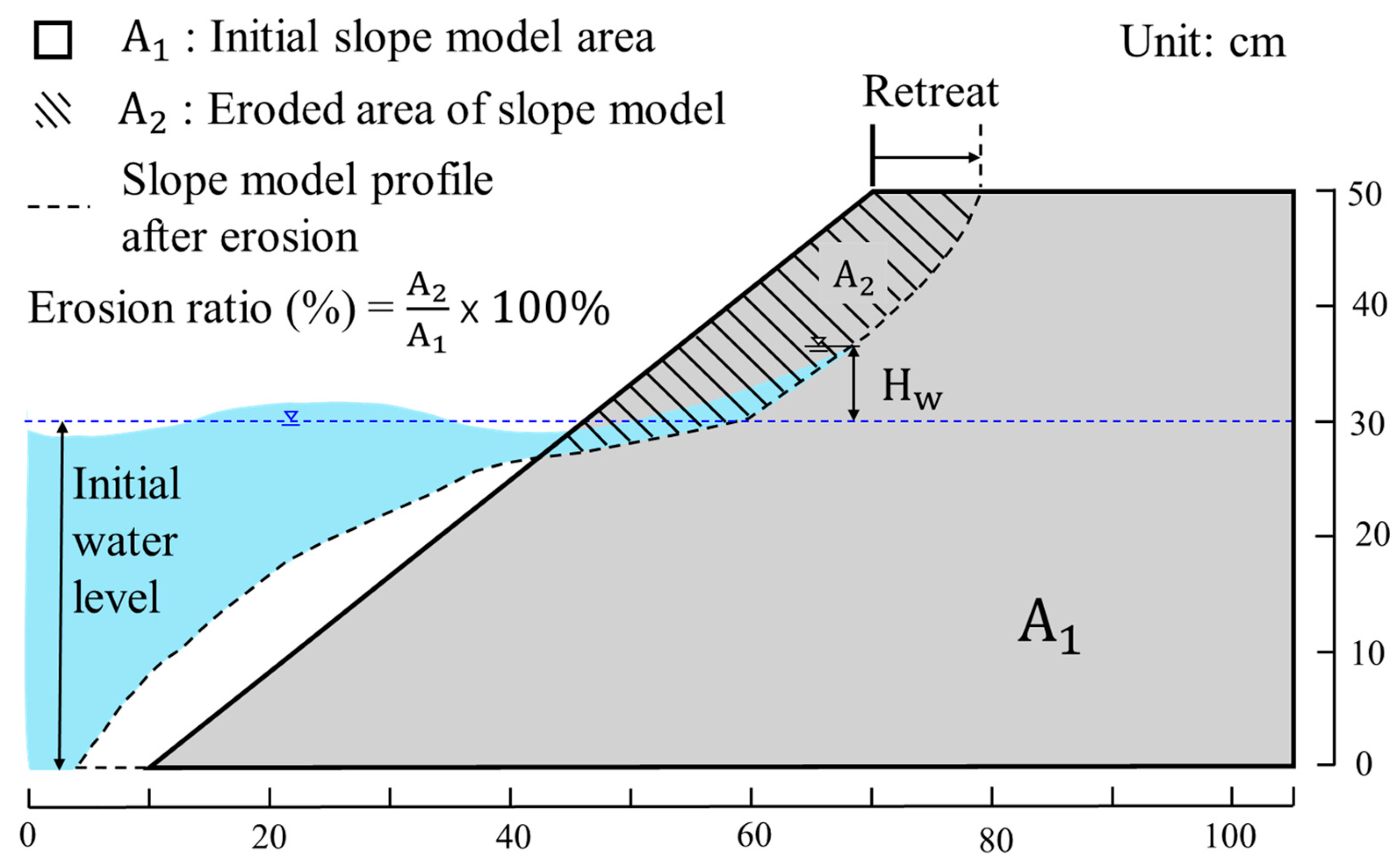
2.3.1. Erosion Ratio, the Run-Up Height of Wave and Retreat of Slope Model

Figure 3 illustrates the assessment methods for erosion ratio, the run-up height of the wave (H_w), and retreat, as described by Peng et al. [26]. A₁ represents the initial surface area of the slope before a test, while A₂ represents the area of the slope materials that has been eroded within the initial slope profile. The run-up height of the wave is the difference in elevation between the highest point reached by the wave as it climbs up the slope and the initial water level. Retreat refers to the reduced distance of the crown of the slope model.

2.3.2. Significant Wave Height, H_s

The definition of significant wave height H_s is the average height of the highest one-third of the waves measured from a set of wave data over a certain period. It generally involves selecting the highest one-third of wave heights and calculating their average to obtain the significant wave height (Equation (1)).

$${\mathrm{H}}_{\mathrm{s}}={\displaystyle \frac{1}{\frac{1}{3}N}}{\sum }_{m=1}^{{\displaystyle \frac{1}{3}}N}{H}_m$$

(1)

For the seismic and acoustic signals, we employed the Hilbert–Huang Transform (HHT, Huang et al. [31]) for analyses. We also calculated the Arias intensity (I_A, Arias [32]) for the seismic signals. Detailed explanations are as follows.

2.3.3. Hilbert–Huang Transform, HHT

The Hilbert–Huang Transform (HHT, Huang et al. [31]) can be used to analyze complex and nonlinear signals. It is particularly useful for interpreting seismic and acoustic signals. HHT consists of Empirical Mode Decomposition (EMD) and Hilbert Transform (HT). EMD decomposes the signal into several Intrinsic Mode Functions (IMFs) and a residual component. The IMFs can then be processed with the HT to obtain a time-frequency representation. This time-frequency spectrum shows the relationship between spectral magnitude (i.e., instantaneous energy), instantaneous frequency, and time, which can help identify the signal characteristics during the erosion process of the slope models. This study conducted the HHT analysis using Visual Signal Ver. 1.6 software (AnCad, Inc., Taipei, Taiwan [33]).

2.3.4. Power Spectral Density

The power spectral density (PSD) can be used to analyze how the power of a signal changes over time within a specific frequency range. The calculation of PSD is referred and modified from Yan et al. [34] as follows (Equation (2)):

$${PSD}_{f_{min}-f_{max}}\hspace{0.17em}\left(t\right)={\displaystyle \frac{1}{{(f}_{max}-f_{min})}}\times {\sum }_{f_{min}}^{f_{max}}\hspace{0.17em}HHT\hspace{0.17em}\left(t,f\right)\hspace{0.17em}df$$

(2)

where $f_{min}$ and $f_{max}$ represent the minimum and maximum frequencies of the analyzed frequency range; “t” represents time; and “HHT (t, f)” represents the time-frequency analysis of the signal using the Hilbert–Huang Transform.

2.3.5. Arias Intensity, I_A

Arias Intensity (I_A, Arias [32]) is a standard measure of seismic intensity. It is defined as the time integral of the square of the acceleration, and the calculation formula is as follows (Equation (3)):

$${\mathrm{I}}_{\mathrm{A}}={\displaystyle \frac{\pi }{2g}}{\int }_{t_1}^{t_2}{\left[a\left(t\right)\right]}^{2}dt$$

(3)

where I_A represents Arias Intensity, “a(t)” is the acceleration as a function of time, and t₁–t₂ is the duration of the seismic event being input. This measure provides a quantitative understanding of the total energy released by the seismicity over its duration, which is particularly useful in assessing the potential damage or effects of seismicity.

2.4. Setup of the Model Tests

A total of 12 tests were performed (

Table 2. Test information of the 12 slope models.

Case	Initial Water Level Hi [cm]	Signifi. Wave Height Hs [cm]	Wave Frequency f [Hz]	Erosion Ratio E [%]	Retreat Re [cm]	Arias Intensity IA [m/s]
Baseline	30.5	1.75	Stage 1: 0.33	0.805	0	0.00298
		2.29	Stage 2: 0.416	0.530	8.226	0.00552
		4.7	Stage 3: 0.5	14.192	20.513	0.00829
1	29.2	1.72	Stage 1: 0.33	0.150	0	0.00301
		2.2	Stage 2: 0.416	0.824	8.639	0.0045
		3.49	Stage 3: 0.5	12.231	18.508	0.00669
2	31.4	1.83	Stage 1: 0.33	0.361	0	0.00338
		2.37	Stage 2: 0.416	0.353	6.298	0.0058
		3.97	Stage 3: 0.5	13.713	20.547	0.00605
3	29.3	2.85	0.833	12.671	22.591	0.01682
4	28.1	4.19		17.649	28.875	0.02747
5	29.4	5.42		18.657	35.064	0.04605
6	29.5	2.95	0.916	13.407	23.138	0.01319
7	30.3	4.22		18.535	25.368	0.0292
8	30.5	5.11		22.359	37.327	0.0487
9	28.6	2.37	1	10.561	15.0311	0.02881
10	28.3	3.82		10.561	26.917	0.04978
11	28.5	4.72		21.131	37.670	0.0751

Note: The erosion ratio and retreat are evaluated stage by stage, and are not cumulatively summed from preceding stages.

). To study the effects of wave height and frequency on the erosion ratio and retreat, we set up a variety of different waves for comparisons and parametrical study. Among them, a test is selected as the Baseline Case for a detailed explanation of various phenomena. The selection of the Baseline Case is based on the completeness of the test result data and the coverage of multiple different wave scenarios. The wave frequencies of the 12 tests ranged from 0.33 Hz to 1 Hz and the significant wave heights ranged from 1.72 to 5.42 cm. Table 2 lists the significant wave height H_s, wave frequency, erosion ratio, retreat, and Arias Intensity for each test.

For comparison, we conducted three tests with the same setup (Baseline Case, Case 1, and Case 2). Varying wave frequencies of 0.33 Hz, 0.416 Hz, and 0.5 Hz were set in the Baseline Case and Cases 1 and 2, which are relatively lower frequencies compared to Cases 3 to 11, which used fixed wave frequencies such as 0.833 Hz, 0.916 Hz, and 1 Hz. To study the effects of different wave heights on the volume of slope erosion and retreat, this study generated waves of three different heights at 0.833 Hz, 0.916 Hz, and 1 Hz.

This study assumed the Froude model law scaling ratio, λ, as 1/80. According to the Froude model law, wave height of prototype = wave height of model/λ, and wave period of prototype = wave period of model/√λ. For the Baseline Case, the significant wave height and frequency/period of model scale, corresponding to prototype scales, are listed in

Table 3. Significant wave height H_s and frequency/period of the model scale (Baseline Case) corresponding to prototype scales.

	Model Scale (Baseline Case)	Prototype Scale	Douglas Sea Scale/State of the Sea
Significant wave height:
Stage 1	1.75 cm	1.4 m	4/Moderate
Stage 2	2.29 cm	1.83 m	4/Moderate
Stage 3	4.7 cm	3.76 m	5/Rough
Wave frequency (Period):
Stage 1	0.33 Hz (3.03 s)	0.037 Hz (27.05 s)	0.037 Hz (27.05 s)
Stage 2	0.416 Hz (2.4 s)	0.047 Hz (21.43 s)	0.047 Hz (21.43 s)
Stage 3	0.5 Hz (2 s)	0.056 Hz (17.86 s)	0.056 Hz (17.86 s)

Note: The Froude model law scaling ratio, λ = 1/80.

. The significant wave height of the prototype in this study is about 1~4 m, and the wave period of the prototype corresponds to around 17~28 s. Waves with heights between 1 and 4 m are typically generated under moderate/rough sea states or slightly stronger storm conditions. The depth of the water in the flume is set to 30 cm, which corresponds to a 24 m depth of the prototype. The height of the slope model was built to 50 cm, which corresponds to a 40 m height of the prototype slope. For reference, in the 4th column of Table 3, we also listed the Douglas Sea Scale and description of wave state according to World Meteorological Organization (Morrisey et al. [35]).

2.5. Test Procedures

The test procedures for this study, which are modified from Peng et al. [26], are as follows:

(1)

Build the slope model, installing sensors and cameras.

(2)

Let the slope model sit for 5 h, allowing the water inside the slope model to naturally drain.

(3)

Once the slope model has settled, pump water from the reservoir into the flume’s headwater until a sufficient volume is reached.

(4)

Begin recording data (water level in the flume, seismic signal, acoustic signal, pore pressure, and video).

(5)

Open the sluice to release water into the flume until the water level reaches 0.3 m.

(6)

Allow the slope model to sit until the water level in the slope model also reaches 0.3 m.

(7)

Turn on the wave maker motor and record the seismic and acoustic signals due to the motor for analyzing its noise.

(8)

Start the test. Turn on the wave maker to create waves that erode the slope model.

(9)

When the slope profile reaches a state of equilibrium, stop the wave maker, and the test ends.

The Baseline Case consists of three stages. The first stage ends when there is minimal change in the slope’s geometry, at which time the wave maker was turned off. When the amplitude of the pore pressure in the slope model decreased and stabilized, the wave maker was started again, marking the beginning of the next stage of the test.

3. Results and Discussion

In this section, the characteristics of pore pressure and seismic and acoustic signals due to wave erosion of the slope are discussed. The results of the Baseline Case are discussed in detail. Two types of wave erosion are defined: impacting and swashing. Impact-type erosion involves wave breaking and splashing, whereas swash-type erosion involves only water moving up and down without breaking and splashing.

The pore pressure signals might indicate how the internal structure of the slope is affected by the waves. An increase in pore pressure can signify that water is being pushed into the slope, potentially destabilizing it and causing material to become loose or displace. Seismic signals can reveal the intensity and the effect of the waves reaching the slope. Different erosion types might show distinctive seismic patterns. The acoustic signals generated by the erosion processes can provide additional insights.

Impact-type erosion with wave breaking and splashing is likely to produce stronger and more abrupt seismic signals compared to the swash type. Impact-type erosion might generate louder and sharper sounds due to the breaking and splashing, while swash-type erosion might have a more consistent and softer soundscape. The evidence is provided in the following. By analyzing these signals and comparing the two types of erosion (impacting and swashing), researchers can gain a deeper understanding of the erosion mechanisms and the effects of different wave actions on slope stability. This analysis is crucial for designing and implementing measures to protect slopes from erosion.

3.1. Overall Interpretations of the Results of Baseline Case

Different wave erosion and slope damage conditions lead to changes in water level, seismic signals, acoustic signals, and pore pressure. To understand the causes of these changes, it is essential first to understand the erosion conditions of the slope. The results of the Baseline Case are divided into three stages, with each stage having the waves set differently in terms of wave height and frequency. In this study, the characteristic of the wave maker is that when a higher wave frequency is set, the wave height also increases accordingly. The limitation of this wave maker causes a correlation between the wave frequency and wave height of the waves produced.

Table 4. The timeline of Baseline Case.

Time [s]	Stage	Procedures/Events	Changes in the Signals/Data
0	-	Test started.	-
250–1180	-	Pumped water into flume until water depth reached 30 cm and waited for the water level in the slope model until steady at 30 cm.	(1) The amplitude of seismic signal increased during 250–280 s. After 280 s, the seismic signal amplitude decreased. (2) The pore pressure of PP1–PP3 and PP4 increased to 0.56 kPa and 0.31 kPa.
1050	-	Turned on the wave maker.	-
1180	Stage 1	Stage 1 started. Wave frequency = 0.33 Hz; Significant wave height = 1.75 cm	The amplitude of the seismic signals and pore pressure increased.
1188–1218		The rapid change in the water level on the slope initiated the onset of instability in the slope model, leading to landslides.	The amplitude of seismic signals of Acc 1 significantly increased.
2380		Stage 1 ended.	The amplitude of the seismic signals and pore pressure decreased.
2380–2520	-	Turned off the wave maker and waited for waves, seismic and acoustic signals, and the pore pressure in the slope model to become stable before Stage 2.	-
2520	Stage 2	Stage 2 started. Turned on the wave maker. Wave frequency = 0.416 Hz; Significant wave height = 2.29 cm	The amplitude of the seismic signals and pore pressure increased.
2528–2562		The rapid change in the water level on the slope initiated the onset of instability in the slope model, leading to landslides.	The amplitude of seismic signals of Acc 1 and Acc 2 significantly increased.
3720		Stage 2 ended.	The amplitude of the seismic signals and pore pressure decreased.
3720–3840	-	Turned off the wave maker and waited for waves, seismic and acoustic signals, and the pore pressure in the slope model to become stable before Stage 3.	-
3840	Stage 3	(1) Stage 3 started. Turned on the wave maker. Wave frequency = 0.5 Hz; Significant wave height = 4.7 cm (2) The accelerometer Acc1 was exposed on the slope model.	(1) The amplitude of the seismic signal, acoustic signals, and pore pressure increased. (2) The amplitude of seismic signals of Acc1 became unreliable.
3849–3862		The rapid change in the water level on the slope initiated the onset of instability in the slope model, leading to landslides.	The amplitude of seismic signals significantly increased.
4391–4692		The wave run-up height rose, and the force of wave impaction increased, which caused the slope model to collapse and also caused the slope to retreat rapidly.	(1) The amplitude of seismic and acoustic signals increased gradually. (2) The pore pressure increased and the amplitude of pore pressure also increased.
4693–4966		The wave run-up height went down, and the force of wave impaction decreased.	(1) The amplitude of seismic and acoustic signals decreased. (2) The pore pressure decreased and the amplitude of pore pressure decreased slightly.
5160		Stage 3 ended. Turned off the wave maker and the whole test ended.	The amplitude of the seismic signal, acoustic signals, and pore pressure decreased.

lists the events and changes of recorded data of the Baseline Case, detailing the changes and observations made at each stage. Figure 4 shows the slope model’s erosion process from Stage 1 to Stage 3.

During Stage 1 (1180 s–2380 s), the slope was eroded by 0.33 Hz waves. The erosion range of the Stage 1 waves was small due to the highest run-up height of wave (H_w) being only about 2.1 cm. The slope damage was limited to the area near the water, forming a wave-cut notch (Figure 4c). Also, because the erosion range of the waves was small, the wave-cut notch did not continue to expand during Stage 1 (Figure 4d,e).

During Stage 2 (2520 s–3720 s), the erosion range of the 0.416 Hz waves was slightly larger (the highest H_w was about 3.4 cm), which enlarged the wave-cut notch (2528 s–2562 s), triggered landslides, and caused the slope to retreat (Figure 4h). However, the erosion range of the waves was still small during Stage 2, so many soil masses remained on the slope after the landslide and were not washed away by the wave backwash (Figure 4i,j).

During Stage 3 (3840 s–5160 s), the waves at 0.5 Hz were higher, and the highest H_w reached about 13.3 cm (the erosion range reached 86.6% of the slope height), causing the slope damage and retreat to exceed that of Stage 1 and Stage 2 (Figure 4l–o). This indicates a significant increase in the impact of wave action on the slope.

The side view of the test during Stage 3 is available for viewing in Video S1 of the Electronic Supplementary Materials, which is presented in a 16× time-lapse format. Supplementary Figure S1 presents a series of side-view images of the slope model from Stage 1 to Stage 3. Supplementary Figures S2 and S3 display the environmental and human noise of seismic and acoustic signals, respectively, for reference.

Figure 5 presents the recorded data from the wave gauges, accelerometers, piezometers, and the microphone. Figure 5a shows the water level in the flume, and by calculating the amplitude of the water level, the significant wave heights H_s for Stage 1, Stage 2, and Stage 3 were found to be 1.75 cm, 2.29 cm, and 4.7 cm, respectively. Figure 5a shows that the water level changes were stable during Stage 1 and Stage 2. However, there was a significant change in the water level amplitude during Stage 3. This might be due to the changes in the slope profile; that is, the changes in the slope profile affected the location of wave reflection. The interaction between incident and reflected waves could have caused resonance phenomena, leading to an increase in wave amplitude during Stage 3.

In general, coastal erosion processes could involve erosion, block falls and mass movements, etc. Usually, wave erosion could first induce undercutting of coastal slope toes near sea level, then trigger block falls if vertical joints are formed due to gravity or even trigger large-scale mass movements when deeper-seated rupture surfaces further developed. These different types of erosion processes could happen in no particular order.

Wave erosion occurs mostly within the range of wave swash, while mass movements can occur from the wave swash zone up to the top of the slope. Block falls may occur when the slope within the wave swash zone becomes flatter and the slope above the wave action zone becomes steeper, resulting in a steep cliff profile. Two primary causes may lead to mass movements. (1) The periodic action of waves and backwash creates fluctuations in pore pressure within the slope, gradually weakening its structure and increasing the likelihood of sliding. (2) Swash and backwash can erode the slope’s surface, resulting in the formation of a wave-cut notch, which further compromises the support for the slope above the notch, ultimately triggering a large-scale slope failure.

Taking the Baseline Case as an example, during the initial stage of erosion, the slope within the wave swash zone is steep, and the primary type of slope failure is sliding. This causes materials to move downslope into the wave swash zone, where they are eroded by the waves (Figure 4a–l). Swash and backwash formed a wave-cut notch on the slope surface (Figure 4c). As the waves continuously act on the slope, their angle within the swash zone gradually becomes less steep and flatter, while the slope above the swash zone begins to develop a steep cliff profile (Figure 4l–o). At this stage, block falls occurred.

Figure 5b–d show the seismic signals from accelerometers Acc 1–3. Figure 5b–d indicate that as the wave height increases, the amplitude of the seismic signals also increases, as seen from Stage 1 to Stage 2, and increases significantly in Stage 3. By comparing the acceleration amplitude of Stage 3 in Figure 5b–d, we learn that the closer the accelerometer is installed to the slope face, the higher the amplitude it records. Additionally, the amplitude difference between Stage 2 and Stage 3 of Acc 1 (Figure 5b) is much higher than that between Stage 2 and 3 of Acc 2 (Figure 5c), also due to Acc 1 being installed closer to the slope face than Acc 2. Similarly, the phenomenon still exists when comparing the amplitudes of Acc 2 and Acc 3. It can be seen that the closer the monitoring position is to the slope, the more obvious the difference in the amplitude of seismic signals caused by different wave erosions. Therefore, if the monitoring position is close to the slope, it may also help identify different wave erosion forces.

The amplitude of seismic signals undergoes significant changes at 1188 s–1218 s, 2528 s–2562 s, and throughout Stage 3. These changes are primarily attributed to slides and the impact of waves. A detailed explanation of how these events influence the seismic signals is provided in Section 3.2 and Section 3.3. The amplitudes of seismic signals from Acc 1, as shown in Figure 5b, were cut off during Stage 3 because the accelerometer was exposed on the slope and can no longer accurately measure the seismicity of the slope.

Figure 5e shows the acoustic signal from the microphone. During Stage 1 and Stage 2, the amplitude of the acoustic pressure mostly oscillates steadily, as the wave action involves less wave breaking and splashing and more swashing. In Stage 3, however, the amplitude of the acoustic signal is amplified due to the increase in wave height and H_w. The increase in wave height and H_w expands the erosion area and changes the type of wave erosion from swash to impact. These changes lead to more frequent wave breaking and splashing, amplifying the sounds during erosion. This suggests that increases in wave height and H_w may result in louder sounds due to wave breaking and splashing, which produces a more pronounced acoustic signal.

Figure 5f–i present the pore pressures at PP1 to PP4. From these figures, the pore pressure remains stable with a constant amplitude envelope during Stage 1 and Stage 2. However, in Stage 3, the pore pressure undergoes significant changes due to the increase in H_w and wave height. Wave resonance might have occurred during Stage 3 due to changes in the profile of the slope, further increasing the wave height.

For Stage 3, the water level WL1, pore pressure PP1–PP4, and run-up height of wave H_w (Figure 6) were compared, as well as the deformed profiles of the slope in Figure 7, to discuss the reasons for the pore pressure changes. Figure 6 marks the timing (t₀–t₆) for which pore pressure changes corresponded to changes in H_w and wave height. Figure 7 shows the change in the slope profile during t₀~t₆, with the slope profile made through video screenshots and manually tracing.

Figure 6a,b show that the water level and pore pressure PP1 follow a similar envelope curve from t₀ to t₃. In these figures, the amplitude of the water level and pore pressure PP1 increase at t₁, followed by a decrease from t₂ to t₃. As the piezometer PP1 was installed near the slope surface (as indicated in Figure 2 and Figure 7), the measurement of pore pressure was directly affected by changes in the water level above it. This indicates that the changes in pore pressure near the slope closely reflect the changes in water level amplitude.

The distances between the piezometers PP1–4 and the slope surface gradually shorten as the slope is eroded (Figure 7). This causes the amplitude of the pore pressure PP1–4 to increase from t₁ to t₂ (Figure 6b–e). As the distance between the piezometers and the slope surface decreases, the influence of the waves on the pore pressure increases, leading to an increase in the amplitude of the pore pressure. Variations in the pore pressure PP2–4 and H_w show similar trends, as indicated by the red arrows in Figure 6c–f. Both increase from t₀ to t₃, then decrease from t₃ to t₄ and from t₅ to t₆. This indicates that as H_w increases, the water level inside the slope also rises due to infiltration, which in turn causes the pore pressure to increase. Conversely, when H_w decreases, the pore pressure also declines. The piezometers installed at different locations show that the ones closer to the slope surface PP1 are primarily influenced by changes in wave height, while those farther from the slope surface PP2–4 are mainly affected by changes in the water level after infiltration.

By observing the pore pressure PP1, which is closest to the slope face, and the variation in H_w from t₃ to t₆, we found similar trends, as indicated by the blue arrows in Figure 6b,f. It can be deduced that the changes in wave height no longer directly affect the pore pressure at PP1. Instead, H_w influenced the pore pressure of PP1 more significantly. This shift is likely because wave erosion caused the slope to deform progressively during t₀ to t₃ (as shown in Figure 7), leading to the dissipation of wave energy. Therefore, as H_w decreases, the water level above the piezometer PP1 also decreases, thereby decreasing the pore pressure of PP1.

In essence, the results demonstrate how the severity of wave erosion at different stages affects slope stability, highlighting the critical role of wave characteristics in the slope erosion process. Important points can be summarized as follows:

(1)

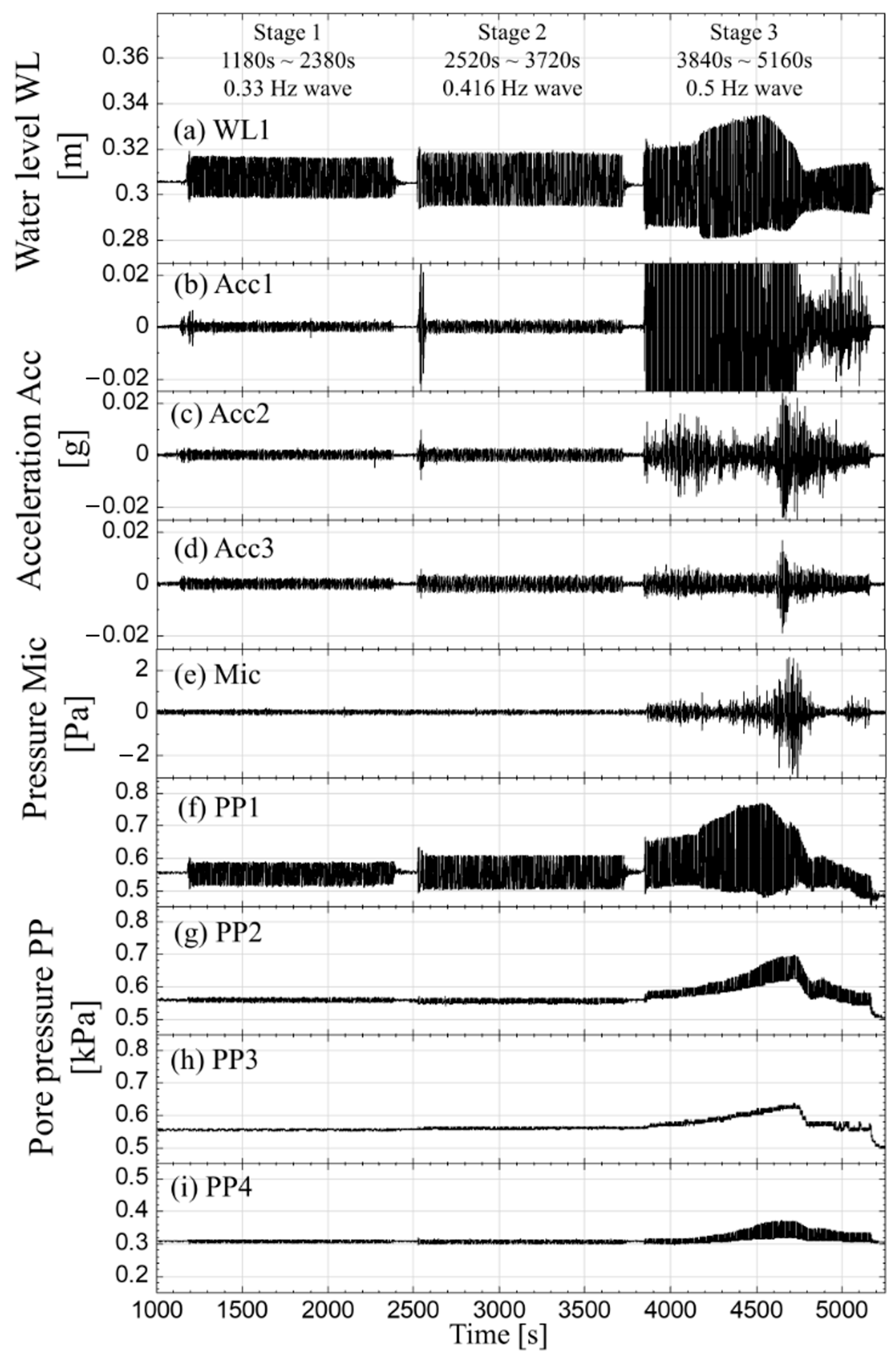
Water height variations: The water height is stable in Stages 1 and 2, but there are significant variations in Stage 3 due to slope profile changes affecting wave reflection.

(2)

Seismic signals: The amplitude of seismic signals increases with wave height, and accelerometers closer to the slope will record higher readings.

(3)

Acoustic signals: The acoustic signals are “quieter” in Stages 1 and 2 and are “louder” with more variations in Stage 3 due to increased wave breaking and splashing.

(4)

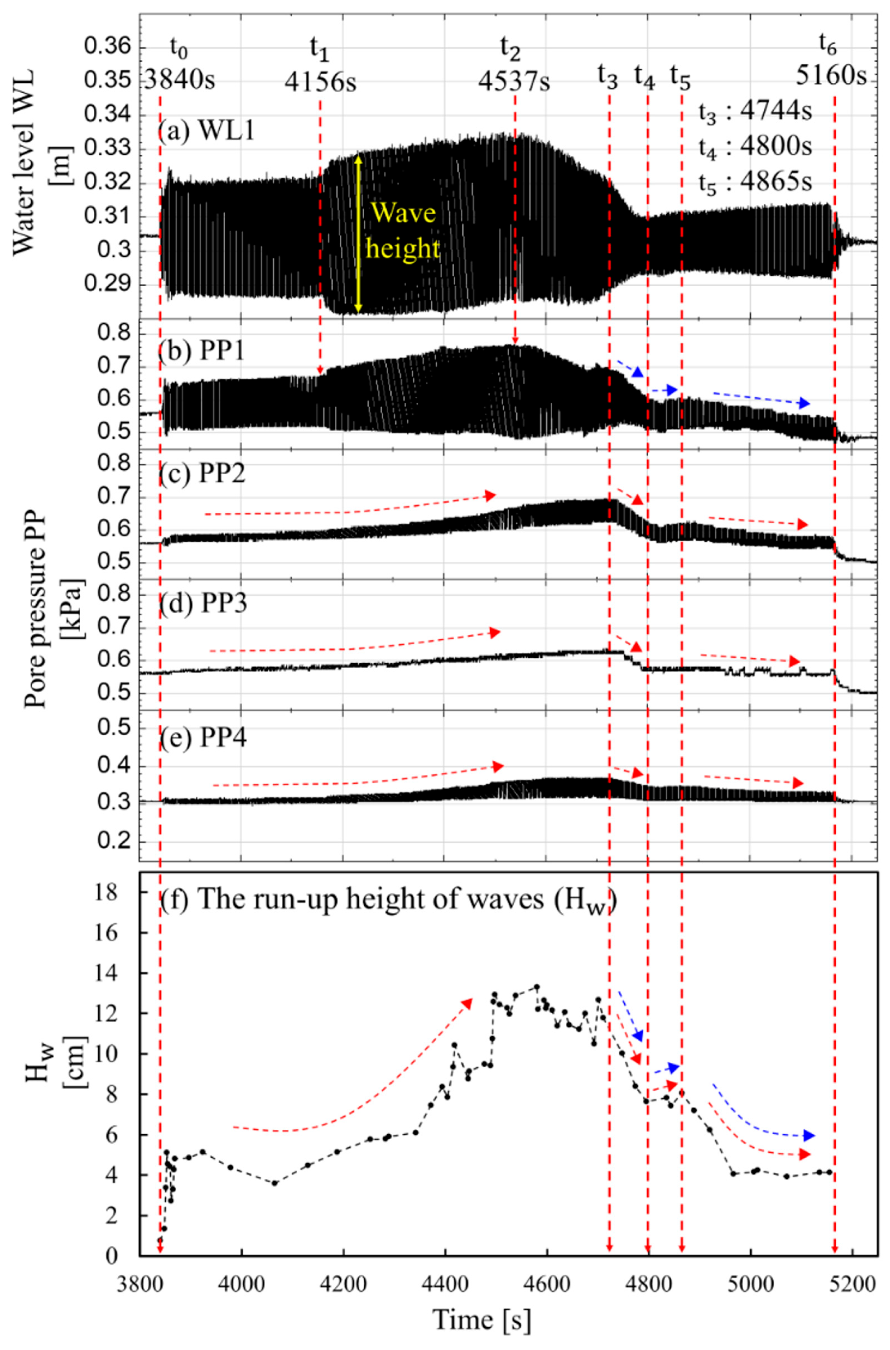
Pore pressures: The pore pressures in the slope are stable in the early stages and have significant changes in Stage 3. Pore pressure changes reflect variations in wave height and H_w, with higher readings when the piezometer is near the eroded slope face. Higher wave height and H_w raise the water level inside the slope, increasing pore pressure.

(5)

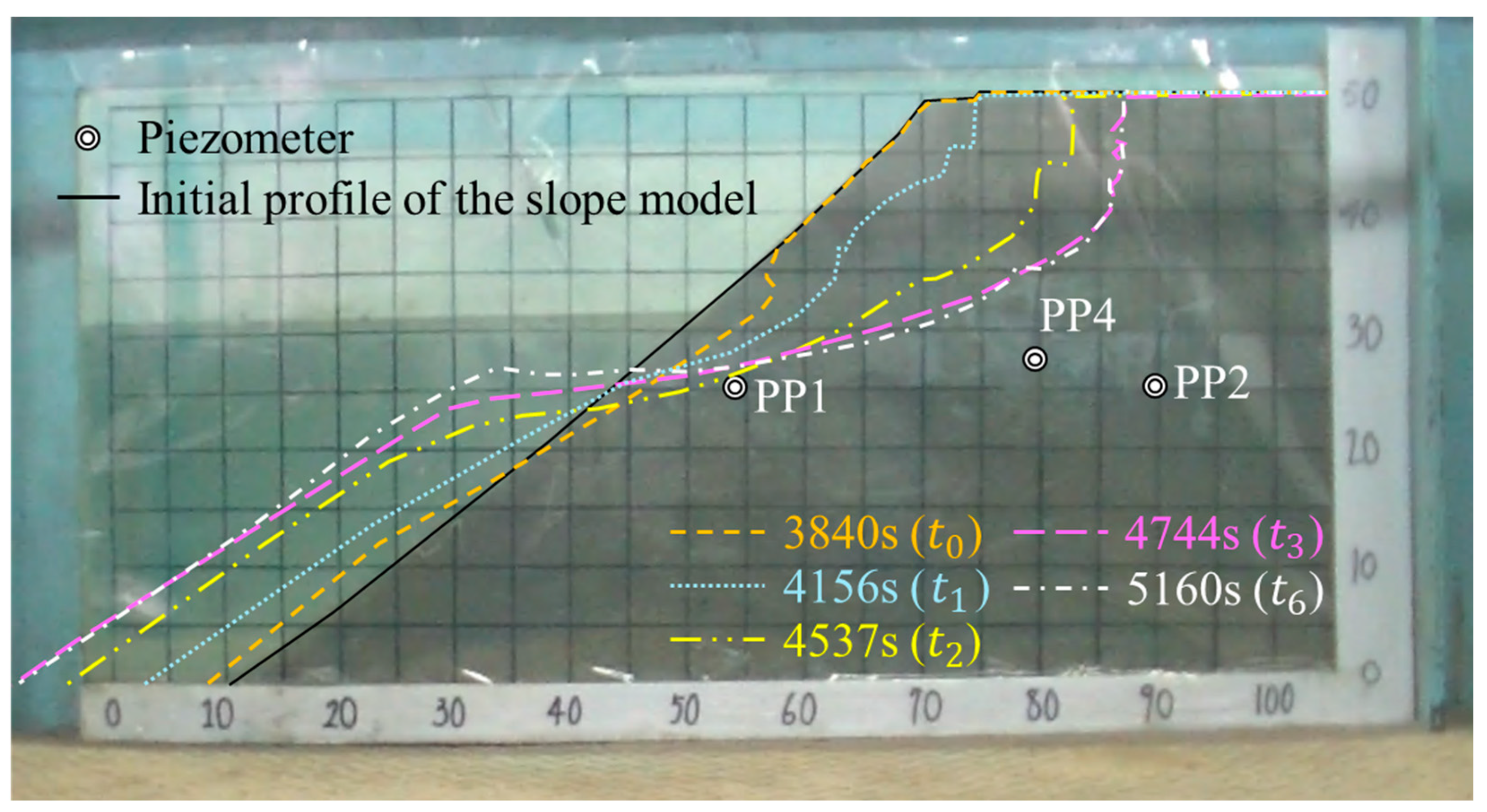
Geometry changes in slope: A change in the slope’s geometry due to wave erosion affects wave energy dissipation, influencing water levels above the piezometers and altering pore pressure.

From the above discussions, the trends between changes in pore pressure and changes in wave height and H_w are similar. The proximity of piezometers to the eroded slope affected the amplitude of pore pressure readings. As the wave height and H_w increased, so did the water level inside the slope, influencing the pore pressure. The geometry changes in the slope due to wave erosion also affected the dissipation of wave energy, thereby influencing the water level above the piezometers and consequently altering the pore pressure.

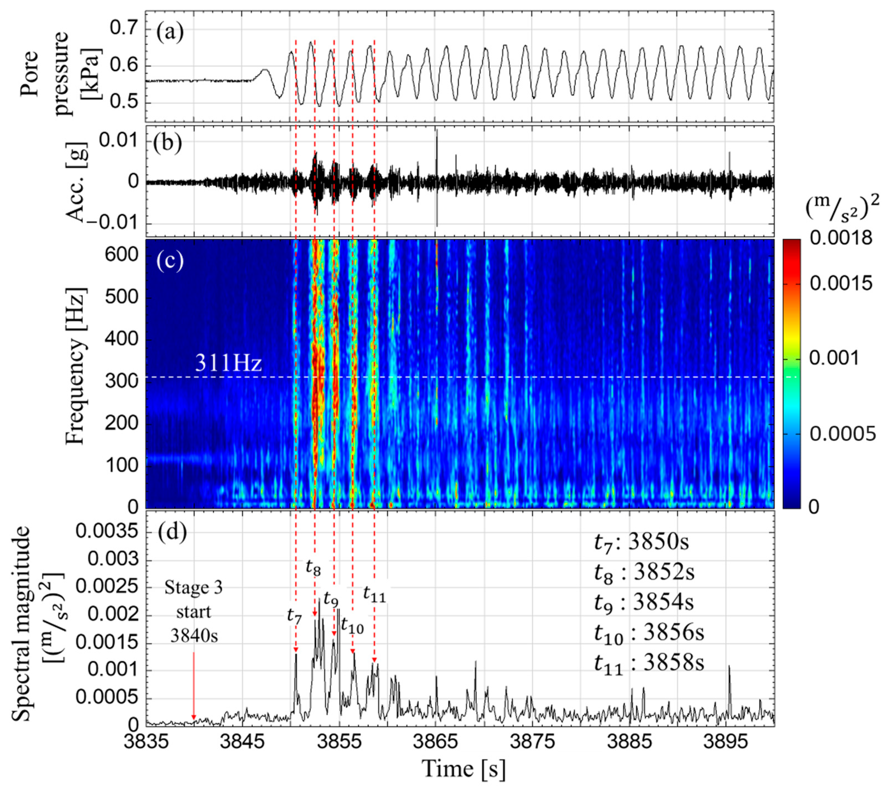
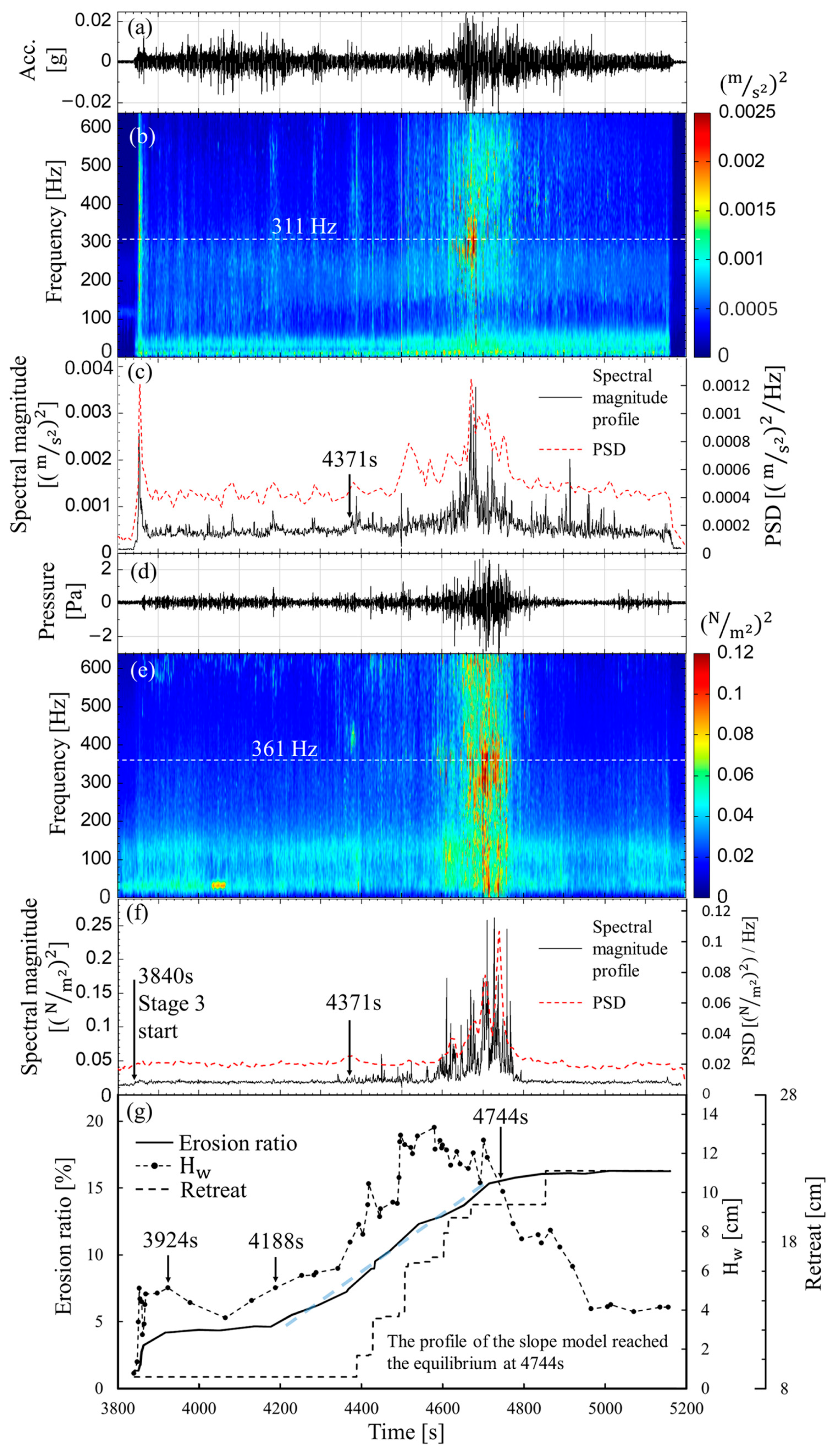
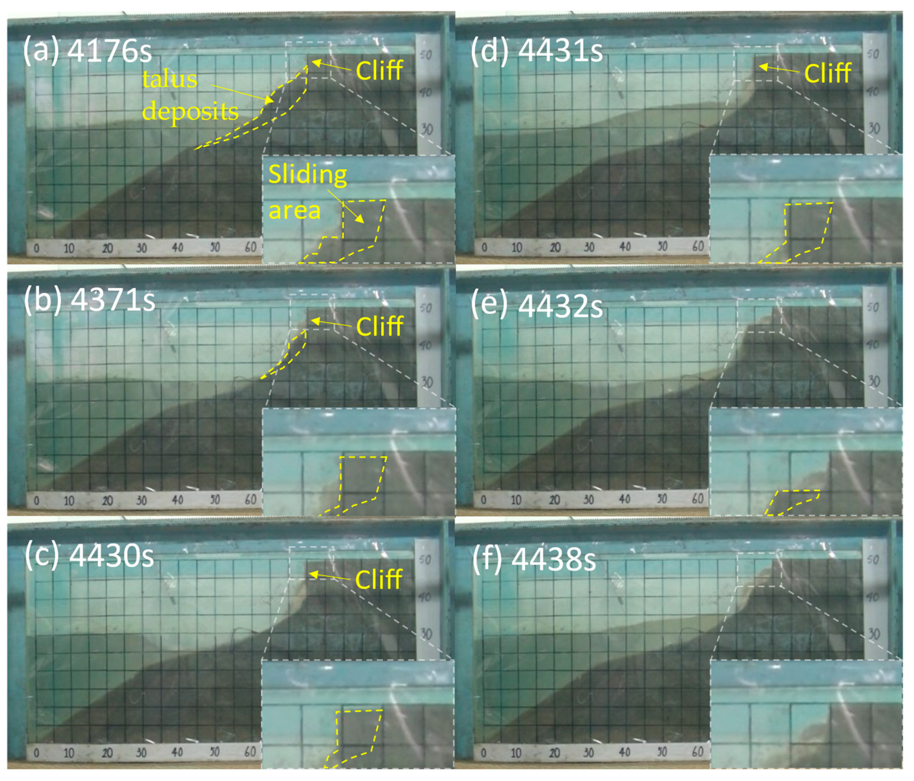
3.2. Characteristics of the Seismic Signals of the Slope Failure (Baseline Case)

Wave erosion leads to changes in the slope profile, and these changes in profile can affect the hydraulic conditions of the waves, which in turn can lead to changes in the scenarios of slope failure. In the Baseline Case, we observed three types of failure scenarios during Stage 3:

(1)

Slope sliding induced by cyclic wave backwash: This occurs when the water retreating back into the ‘sea’ (backwash) pulls material from the slope with it, leading to sliding. The cyclic nature of the waves can cause repeated sliding events.

(2)

Re-sliding of the previously slid soil mass induced by wave swash: Swash refers to the water rushing up the slope after breaking. This scenario involves the reactivation and further movement of soil masses that had previously slid down but not completely detached or been washed away.

(3)

Slope collapse induced by wave impact: This refers to the failure and sudden movement of a portion of the slope due to the force of the waves impacting the slope, often accompanied by breaking and splashing.

To understand the characteristics of the seismic signals of slope failure under these three scenarios, we selected seismic signals from three periods for analysis, specifically 3835 s–3900 s, 3800 s–4680 s, and 4500 s–4600 s, and we discuss them in detail as follows.

Figure 8 presents the pore pressure PP1, seismic signal Acc 2, time-frequency spectrum, and spectral magnitude profile from 3835 s to 3900 s. The PP1 piezometer, being close to the slope surface, can measure changes in the water level above it. In Stage 3, wave generation starts at 3840 s, and the amplitude of both the PP1 pore pressure (Figure 8a) and the seismic signal Acc 2 (Figure 8b) begin to increase after this time. During 3850 s–3858 s, the slope experienced five slides. The yellow and red energy traces in the time-frequency spectrum (Figure 8c) are caused by the slope sliding. Since the energy traces are approximately concentrated around 311 Hz, we plotted the spectral magnitude profile of 311 Hz, as shown in Figure 8d. The 311 Hz is auxiliary, determined by using Fourier Transform to convert the signal from the time domain to the frequency domain, and then the frequency centroid is calculated to determine the frequency where the energy is concentrated. Figure 8d marks the times (t₇–t₁₁) when the spectral values rise, which also represent the moments of slope sliding. Comparing Figure 8a with Figure 8d, we observe that the peaks in spectral values (t₇–t₁₁) correspond to decreases in PP1 pore pressure, indicating that slope sliding occurs during backwash when the water level on the slope face drops. Therefore, as the waves cyclically backwash, rapid drawdown might also be one of the causes of slope sliding. Figure 9 is a set of snapshots during 3840 s–3858 s, with the red dashed line representing the area of slope sliding. The processes of t₇–t₁₁ sliding and timing can be viewed from Video S2.

Figure 10 presents the seismic signal, time-frequency graph, spectral magnitude profile of Acc 2, and retreat from 3800 s to 4680 s. Since the energy traces were also concentrated around 311 Hz during 3835 s–3900 s, we plotted the spectral magnitude profile at 311 Hz. The 311 Hz is auxiliary, selected by using Fourier Transform to convert the signal from the time domain to the frequency domain, and then calculate the frequency centroid where the energy is concentrated. Figure 10c shows spectral peaks at t₁₂–t₁₆, which are due to slope sliding (t₁₂–t₁₅) and collapse (t₁₆). Because collapse causes the slope to retreat, the retreat distance increases at t₁₆ (Figure 10d). Figure 11a presents photos of the landslide (t₁₂–t₁₅) and collapse (t₁₆) during 4025 s–4388 s. During the test, the upper part of the slope gradually formed a cliff (Figure 11a) due to wave erosion. The soil accumulated on the cliff’s surface, already loosened by previous sliding, was prone to re-sliding due to wave swash (Figure 11a–d). As the soil on the upper cliff was gradually carried away by backwash, the cliff lost its protection, making it susceptible to collapse due to wave erosion (Figure 11e). The processes of t₁₂–t₁₅ sliding and t₁₆ collapsing can be viewed from Videos S3 and S4. These videos provide a visual representation of the slope’s transformation and re-sliding events.

Figure 12 presents the seismic signal Acc 2, time-frequency graph, and spectral magnitude profile from 4500 s to 4600 s. During this period, the force of the wave impact on the slope was substantial, and significant sounds of wave impact can be heard from the experimental video. Figure 12b shows faint blue vertical energy traces in the time-frequency spectrum, which are caused by wave impact on the slope. Figure 12c marks the times of slope collapse (t₁₇–t₂₂) that were observed from the test video, with spectral value peaks at t₁₈, t₂₀, and t₂₂. The collapses at t₁₇, t₁₉, and t₂₁ are hard to recognize from Figure 12c, which may due to the very small energy and the characteristic of the seismic frequency content of the collapses. Corresponding photos from the experiment (Figure 13c,e,g) show that the upper cliff of the slope had larger collapses at t₁₈ and t₂₀, resulting in greater vibrations. The collapse event at t₂₂ was recorded due to the falling soil mass being closer to the sensor Acc 2. There are no peaks in the spectral values at t₁₇, t₁₉, and t₂₁, possibly because the volume of the collapse was small, or the locations of the falling soils were too far from the sensor to be reflected in the seismic signal. During the rapid retreat of the slope, the force of the wave impact was stronger, creating many energy traces in the time-frequency spectrum (Figure 12b), making it more challenging to identify collapse events. However, during periods of wave swash, there are fewer energy traces from wave impact on the slope; therefore, the collapse event can be identified. The processes of t₁₇–t₂₂ collapse can be viewed in Video S5.

The above discussion provides a detailed account of how wave-induced changes in slope profiles lead to varied forms of slope failure, utilizing seismic signal analysis to understand the complex interactions between wave action and slope stability. We believe that the ultimate causes of slope failure due to wave erosion are cyclic processes, such as swash, backwash, rapid drawdown, and toe erosion. As the soil masses on the upper cliff of the slope are gradually carried away by backwash, the cliff becomes prone to collapse due to wave erosion. If a collapse occurs under the conditions of wave impact on the slope, the energy traces of the collapse on the time-frequency spectrum may be obscured or interfered with by the traces of wave impact energy. This complex interplay of wave forces shows that slope stability is not just a matter of static geological conditions but is significantly influenced by the dynamic forces exerted by waves. These forces cyclically and progressively weaken the slope, leading to various types of failure over time. Monitoring the seismic signals and analyzing the time-frequency spectrum and spectral magnitude profile provide valuable insights into the dynamic wave actions and slope failure processes.

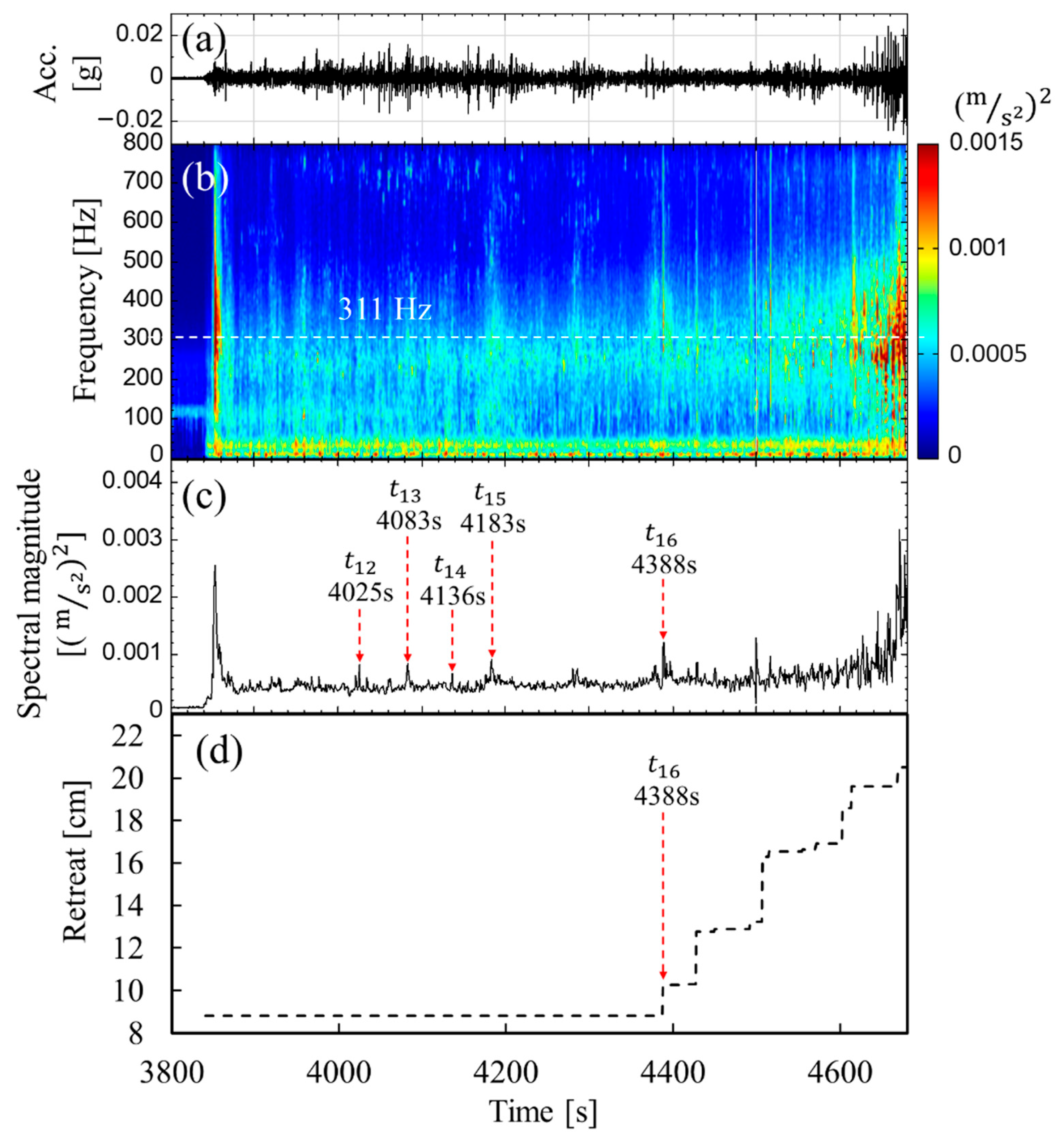
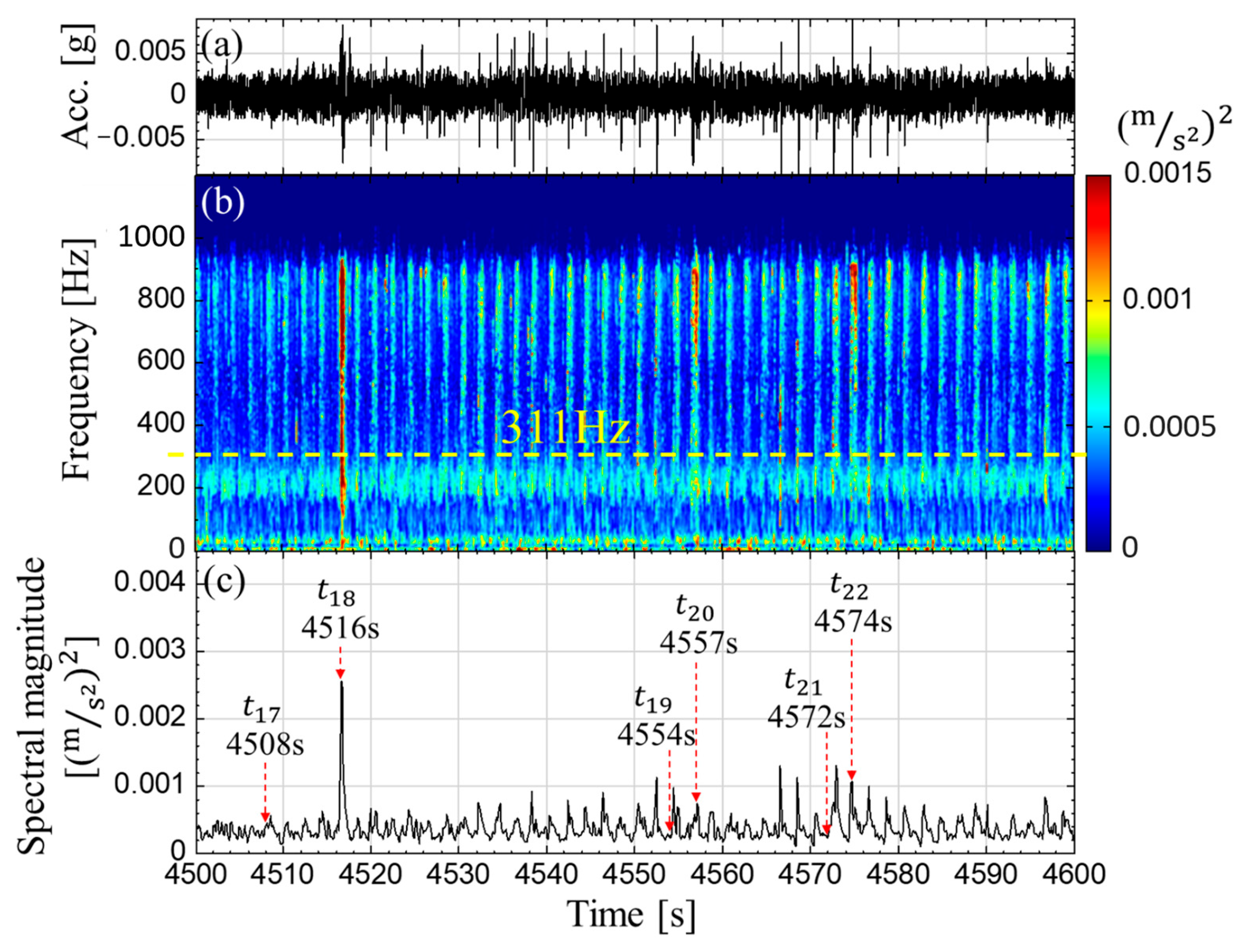
3.3. Slope Erosion Versus Seismic Signals and Acoustic Signals (Baseline Case)

In the Baseline Case, significant changes in seismic and acoustic signals were observed during Stage 3, compared to Stages 1 and 2. Observing Figure 4 reveals that the majority of slope damage due to wave erosion occurs in Stage 3. Figure 14a–f present the analysis results of seismic and acoustic signals. To understand the reasons behind the changes in the signals, we examined the variations in spectral magnitude and Power Spectral Density (PSD) (Figure 14c,f) and compared them with the erosion ratio, run-up height of waves (H_w), and retreat (Figure 14g). We also correlated these with video observations of the wave erosion behavior and slope damage over time. Figure 14b is the time-frequency spectrum of the seismic signal, and the spectral magnitude profile of 311 Hz is shown in Figure 14c. Figure 14e is the time-frequency spectrum for the acoustic signal; because the red and yellow energy traces are concentrated around 361 Hz during 4600 s–4800 s, we took the 361 Hz cross-section of the time-frequency spectrum, obtaining the spectral magnitude profile for the acoustic signal (Figure 14f). To observe the changes in energy from 0–600 Hz, we calculated the PSD for seismic and acoustic signals, respectively (Figure 14c,f).

During 3840 s–3924 s, the slope experienced sliding, which caused the spectral magnitude and PSD of the seismic signal to rise (Figure 14c), but there was no significant rise in the spectral values and PSD of the acoustic signal (Figure 14f). This may be because the sound of soil particles rubbing against each other and the sound of wave erosion on the slope was relatively quiet during slope sliding.

During 4188 s–4371 s, both H_w and the erosion ratio rose (Figure 14g), indicating that as H_w increased, the range of wave erosion also increased. This led to more soil being eroded away by the waves, raising the erosion ratio. Generally, it is expected that as the erosion ratio rises, both seismic and acoustic signals would increase. However, our test showed that the spectral magnitude and PSD of the signals (Figure 14c,f) did not increase correspondingly with the erosion ratio (Figure 14g). This is because the soil carried away by wave backwash during 4188 s–4371 s was just the soil that previously slid and remained on the slope surface. These soil masses were loosely structured, and the wave swash could erode and carry them away without generating impact. This is also why, during 4188 s–4371 s, the spectral magnitude and PSD of seismic and acoustic signals did not rise, while the erosion ratio continued to increase.

Figure 15 shows the changes in slope profile during 4176 s–4438 s. According to Figure 15a–c, as the waves erode, the upper part of the slope gradually forms a steep cliff due to the decreasing amount of “talus deposits”. The term “talus deposit” refers to materials from the upper slope that accumulate on the surface after sliding and/or collapsing, without being backwashed into the water. As shown in Figure 15a, the talus deposits covering the slope surface had previously experienced sliding but had not yet been eroded away due to the limited range of wave erosion. Because this talus deposit had experienced sliding, its structure was loose and easily eroded away as the range of wave erosion increased due to H_w rising (Figure 15b), even if the force of wave erosion was weak. This helps further explain why the energy of seismic and acoustic signals did not increase at high erosion ratios during 4188 s–4371 s. As most of the talus deposits were eroded away (Figure 15a,b) during 4176 s–4371 s, waves subsequently began to erode previously unaffected areas of the slope. Since the type of wave erosion began to change from swash to impact after 4371 s, this caused the spectral magnitude and PSD of both seismic and acoustic signals to begin to rise (Figure 14c,f).

During 4600 s–4800 s, the wave erosion was in the form of impact, and the sound of wave erosion was noticeably louder during this period. This illustrates that the yellow and red energy traces in the time-frequency spectrum (Figure 14b,e) are caused by wave impact. Compared to swash-type wave erosion, impact-type wave erosion causes more significant vibrations on the slope and also produces louder sounds. We found that as H_w decreased, the PSD of both signals also decreased. Observing Figure 14c,f,g, during 4600 s–4800 s, the PSD of the seismic signal began to decrease at 4670 s, followed by a decrease in H_w at 4701 s, and finally, the PSD of the acoustic signal decreased at 4739 s. The timing differences of approximately 1–2 min are relatively minor compared to the entire duration of Stage 3, and the times of decline for the three factors (PSD of the seismic signal, PSD of the acoustic signal, and H_w) are closely aligned. This reflects that a decrease in H_w reduces both the force of wave erosion on the slope and the energy of the sound.

Figure 14g shows that H_w first decreases and then increases, and the erosion ratio changes little during 3924 s–4188 s. Generally, each time H_w surpasses its previous maximum value, it indicates that a new range of the slope is being eroded. During 4188–4744 s, although H_w gradually rose, the erosion ratio only steadily increased. This indicates that the erosion rate during this duration is about the same, because the slope of the curve of the erosion ratio is approximately the same (as the light blue dashed line). So, although H_w increased, the erosion rate did not correspondingly increase. After 4744 s, the erosion ratio slowly changed from 16% to the final 16.5%. This indicates that after 4744 s, the force of wave impact on the slope had significantly reduced, causing only a small amount of erosion, and the erosion rate approached zero. This caused the curve of the erosion ratio to gradually level off, and the slope’s profile tended toward a steady state. It is defined such that the slope reaches a state of equilibrium profile.

As shown in Figure 15a–c, as the talus deposits gradually decreased due to swash, the top of the slope began to gradually form a cliff. In this process, the disappearance of the protection from the talus deposits relative to the top of the cliff meant that the cliff had a tendency to slide; for example, the sliding area is the yellow dashed zone shown in Figure 15a–e. When the cliff’s profile is formed and the range of wave erosion can affect the stability of the cliff, the top of the cliff is prone to sliding or collapsing (Figure 15d–f).

This section can be summarized as follows. (1) Intense wave swash and impact on the slope surface will increase seismic and acoustic energy. (2) Despite increases in H_w and erosion ratio, the spectral values and PSD of seismic and acoustic signals did not rise correspondingly. This was attributed to the erosion of loosely structured soil that had previously slid and remained on the slope without impact. (3) As erosion changed from swash to impact, there was a noticeable increase in the spectral values and PSD of both seismic and acoustic signals. (4) Wave erosion occurred through impact, producing louder sounds and greater seismic activity than swash erosion. (5) Despite the gradual increase in H_w, the erosion rate remained roughly the same, and the erosion rate did not increase correspondingly with H_w. (6) The turning points of the decrease in vibration and sound energy indicate that the force of wave erosion on the slope began to gradually diminish, due to the decrease in the run-up height of the wave (H_w).

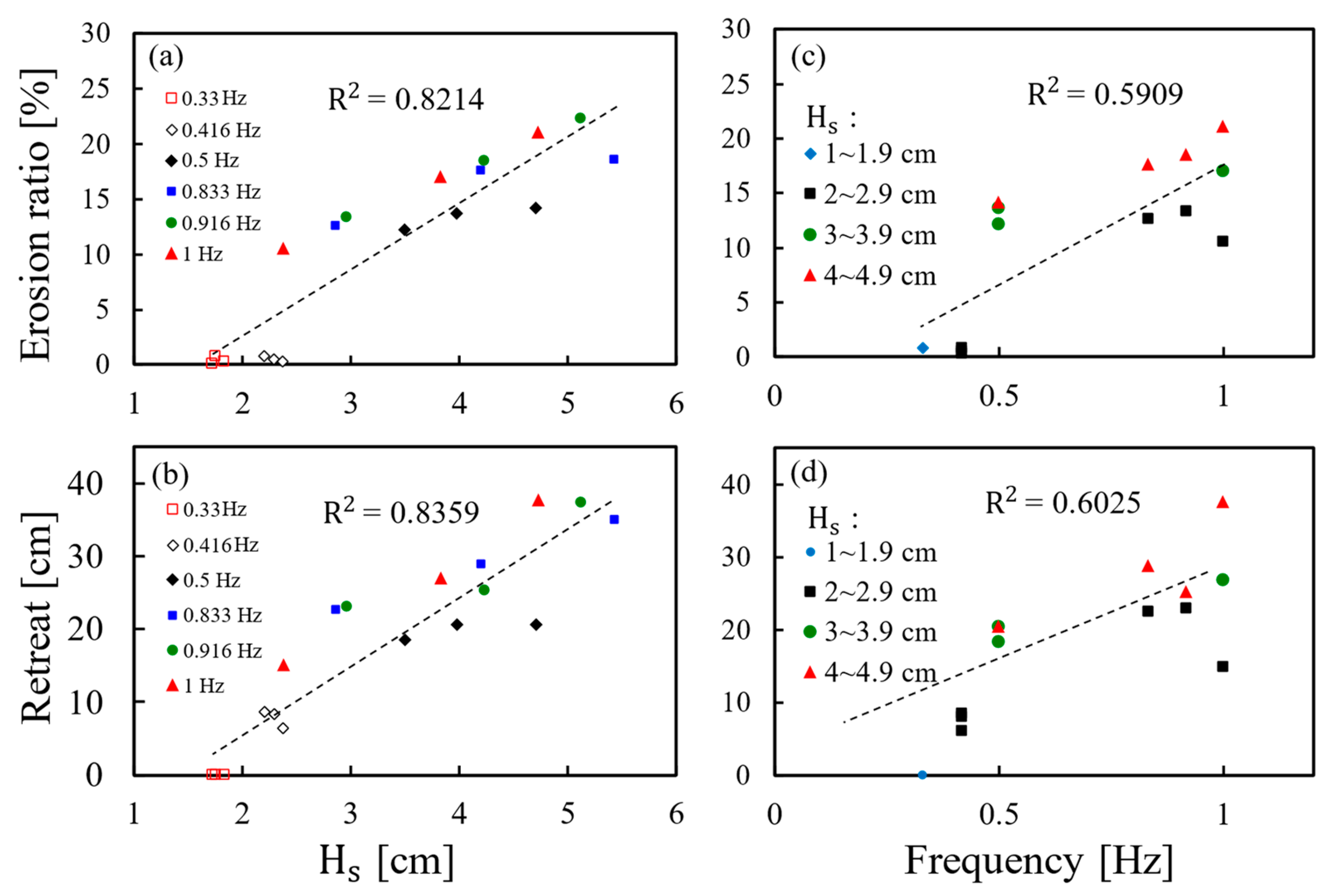
3.4. Parametric Study of Influence of Significant Wave Height H_s and Wave Frequency on the Erosion Ratio, Retreat, and Arias Intensity I_A

This section discusses the influence of significant wave height H_s and wave frequency on the erosion ratio, retreat, and I_A by comparing the test results from the Baseline Case and Cases 1–11. The significant wave height H_s is discussed instead of the wave height because the wave height during Stage 3 in the Baseline Case, Case 1, and Case 2 varied too much. Table 2 lists the outcomes of the erosion ratio, retreat, and I_A. These outcomes are evaluated based on the state of the equilibrium profile and a duration of 900 s since the wave maker started. The results are plotted in Figure 16 and Figure 17 with trend lines.

According to Figure 16a, there is a noticeable correlation between the erosion ratio and H_s (significant wave height); even under the same wave frequency conditions, a higher H_s typically indicates a higher erosion ratio. However, under the wave action of 0.33 and 0.416 Hz, the erosion ratio is relatively smaller due to the lower H_s. This underscores the significant impact of H_s on the erosion ratio. Figure 16b illustrates the relationship between retreat and H_s. Under the same wave frequency conditions, a higher H_s results in a longer retreat distance. With 0.33 Hz wave action, the retreat is almost negligible, as the lower H_s restricts erosion primarily to the slope surface. In contrast, under the influence of 0.416 Hz waves, due to the higher H_s, the retreat is notably longer than that at 0.33 Hz. The trend lines derived from linear regression analysis in Figure 16a,b, with an R² value of approximately 0.8, demonstrate the strength of these correlations. Figure 16c shows that as wave frequency increases, regardless of whether the H_s is the same or not, the slope’s erosion ratio exhibits an upward trend. Additionally, Figure 16c also reveals that a higher H_s is associated with a relatively higher erosion ratio. Figure 16d indicates that higher wave frequencies lead to an increase in the retreat distance of slopes, a trend that is consistent across different H_s values. The linear regression analysis for Figure 16c,d shows trend lines with an R² value of about 0.6. These data suggest that the impact of H_s on the erosion ratio and retreat is greater than that of wave frequency.

Figure 17 reveals a significant trend; the higher the erosion ratio, the greater the resulting I_A and seismic energy. This finding can be an important future application for seismic monitoring and early warning of slope erosion or collapse and sliding under wave actions. For example, if a seismic sensor detects a higher amount of seismic energy, it may indicate that the slope is experiencing more severe erosion.

There are various methods to mitigate erosion effects, including hardware engineering measures (such as breakwaters and sea walls), “software” measures (like beach nourishment and vegetation planting), and methods to reduce wave energy (such as underwater dissipaters and artificial reefs). The results of this study could be used to help assess the erosion conditions of coastal slopes, aiding in the formulation of strategies to mitigate wave erosion effects.

4. Conclusions

This study conducted flume tests on wave erosion of slope models, utilizing various wave frequencies and heights for the tests. The data measured during the experiments included wave water levels, seismic and acoustic signals, and pore pressure. We also analyzed the slope model’s erosion ratio, slope retreat, and the run-up height of the wave (H_w) through image analysis. The study found that at least three factors influence the seismic and acoustic energy of wave erosion, including (1) wave height, (2) waves swashing and impacting the slope, and (3) the run-up height of the wave. This phenomenon could be applied and is promising for issuing near-shore slope failure warnings. The main conclusions are as follows:

• Piezometers and seismic sensors should be installed as close to the slope surface as possible but also positioned to avoid exposure by erosion. This placement allows for the measurement of more significant signals. The variation in wave height strongly affects the amplitude of pore pressure near the slope surface. The higher the wave height, the greater the amplitude of the pore pressure, indicating stronger wave erosion forces. Therefore, sensors should be placed as close to the slope face as possible in applications to assess changes in wave height and the condition of wave erosion.
• As the run-up height of the wave (H_w) rises, the pore pressure generally also increases, even if the piezometers are installed a bit away from the slope surface. The increase in pore pressure can be used as an indicator of the increase in the H_w, reflecting the enlargement of wave erosion on slopes. As waves gradually erode the slope surface, the amplitude variation in pore pressure increases, serving as an indicator that the slope has undergone further erosion.
• When waves backwash cyclically, the rapid drawdown phenomenon may induce sliding of the slope.
• Generally, when waves intensely swash and impact the slope surface, seismic and acoustic energy traces in the time-frequency spectrum will be very obvious. If a collapse occurs while the wave impacts the slope, the energy traces of the collapse in the time-frequency spectrum can easily be masked by the energy traces of the impacting waves.
• With the transition of erosion from swash to impact, a marked rise in both the spectral magnitude and Power Spectral Density (PSD) of seismic and acoustic signals was observed. The impact mode of wave erosion generated louder sounds and more significant seismic energy compared to that from swash erosion.
• Sometimes, even when H_w and the erosion ratio increase, the spectral values and PSD of the seismic and acoustic signals may not increase correspondingly. This is due to previously slid loose soils being swashed without being impacted. Even though the H_w gradually increased, the erosion rate remained roughly the same; that is, the erosion rate did not increase correspondingly with H_w. As the H_w decreased, the turning point where seismic and acoustic energy declined indicates that the force of wave erosion on the slope began to diminish gradually.
• Wave height has a greater influence on erosion and retreat compared to wave frequency, based on the R² values from the linear regression.
• Arias Intensity (I_A) and erosion ratio increased exponentially. Therefore, when I_A due to wave action can be obtained for a slope, there is great potential for I_A to be applied in estimating the erosion ratio for that slope.

Due to the small scale of the tests, all seismic signals generated during the small-scale model tests can be easily recorded. However, if significant human or environmental noise is present and the source of this noise is close to the sensors, the seismic signals we intend to monitor may be easily obscured. Natural slopes are usually composed of a variety of materials, such as gravels, sands, silts, and clay, and rocks whose properties can affect wave propagation and lead to significantly different signal patterns. Therefore, further study could consider investigating slopes with various geological materials. The direction of wave impact and the direction of slope sliding may be identified by seismic signals in specific directions. Therefore, in the future, attempts can be made to measure the multi-directional seismic signals of slopes.

References

1. Bao, Y.; Tang, Q.; He, X.; Hu, Y.; Zhang, X. Soil erosion in the riparian zone of the Three Gorges Reservoir, China. Hydrol. Res. 2015, 46, 212–221. [Google Scholar] [CrossRef]
2. Cleary, P.W.; Prakash, M.; Mead, S.; Lemiale, V.; Robinson, G.K.; Ye, F.; Ouyang, S.; Tang, X. A scenario-based risk framework for determining consequences of different failure modes of earth dams. Nat. Hazards 2015, 75, 1489–1530. [Google Scholar] [CrossRef]
3. Lopez-Saez, J.; Corona, C.; Morel, P.; Rovéra, G.; Dewez, T.J.B.; Stoffel, M.; Berger, F. Quantification of cliff retreat in coastal Quaternary sediments using anatomical changes in exposed tree roots. Earth Surf. Process. Landf. 2018, 43, 2983–2997. [Google Scholar] [CrossRef]
4. Sajinkumar, K.S.; Kannan, J.P.; Indu, G.K.; Muraleedharan, C.; Rani, V.R. A composite fall-slippage model for cliff recession in the sedimentary coastal cliffs. Geosci. Front. 2017, 8, 903–914. [Google Scholar] [CrossRef]
5. Severson, J.P.; Nawrot, J.R.; Eichholz, M.W. Shoreline stabilization using riprap breakwaters on a Midwestern reservoir. Lake Reserv. Manag. 2009, 25, 208–216. [Google Scholar] [CrossRef]
6. Zhu, C.; Peng, J.; Jia, Y. Marine geohazards: Past, present, and future. Eng. Geol. 2023, 323, 107230. [Google Scholar] [CrossRef]
7. Vallejo, F.M. Bluff response to wave action. Eng. Geol. 1988, 26, 1–16. [Google Scholar] [CrossRef]
8. Shipman, H.M. Coastal Bluffs and Sea Cliffs on Puget Sound, Washington. In Formation, Evolution, and Stability of Coastal Cliffs–Status and Trends; Hampton, M.A., Griggs, G.B., Eds.; U.S. Geological Survey Professional Paper No. 1693; U.S. Geological Survey: Reston, VA, USA, 2004. [Google Scholar]
9. Hampton, M.A.; Griggs, G.B.; Edil, T.B.; Guy, D.E.; Kelley, J.T.; Komar, P.D.; Mickelson, D.M.; Shipman, H.M. Processes that Govern the Formation and Evolution of Coastal Cliffs. In Formation, Evolution, and Stability of Coastal Cliffs–Status and Trends; Hampton, M.A., Griggs, G.B., Eds.; U.S. Geological Survey Professional Paper No. 1693; U.S. Geological Survey: Reston, VA, USA, 2004. [Google Scholar]
10. Kawamura, S.; Miura, S. Stability evaluation of slope with soft cliff. Int. J. Geotech. Eng. 2012, 6, 185–191. [Google Scholar] [CrossRef]
11. Ji, F.; Shi, Y.; Li, R.; Zhou, H.; Wang, D.; Zhang, J. Progressive geomorphic evolution of reservoir bank in coarse-grained soil in East China—Insights from long-term observations and physical model test. Eng. Geol. 2021, 281, 105966. [Google Scholar] [CrossRef]
12. Qin, Z.; Lai, Y.; Tian, Y. Study on failure mechanism of a plain irrigation reservoir soil bank slope under wind wave erosion. Nat. Hazards 2021, 109, 567–592. [Google Scholar] [CrossRef]
13. Ozeren, Y.; Wren, D.G.; Reba, M.L. Wave-induced erosion of soil embankment in laboratory flume. J. Hydraul. Eng. 2021, 147, 04021011. [Google Scholar] [CrossRef]
14. Morales, T.; Clemente, J.A.; Mollá, L.D.; Izagirre, E.; Uriarte, J.A. Analysis of instabilities in the Basque Coast Geopark coastal cliffs for its environmentally friendly management (Basque-Cantabrian basin, northern Spain). Eng. Geol. 2021, 283, 106023. [Google Scholar] [CrossRef]
15. Alberti, S.; Olsen, M.J.; Allan, J.; Leshchinsky, B. Feedback thresholds between coastal retreat and landslide activity. Eng. Geol. 2022, 301, 106620. [Google Scholar] [CrossRef]
16. Carpenter, N.E.; Dickson, M.E.; Walkden, M.J.A.; Nicholls, R.J.; Powrie, W. Effects of varied lithology on soft-cliff recession rates. Mar. Geol. 2014, 354, 40–52. [Google Scholar] [CrossRef]
17. Castedo, R.; Fernández, M.; Trenhaile, A.S.; Paredes, C. Modeling cyclic recession of cohesive clay coasts: Effects of wave erosion and bluff stability. Mar. Geol. 2013, 335, 162–176. [Google Scholar] [CrossRef]
18. Wang, L.; Li, Q.; Chen, Y.; Wang, S.; Li, X.; Fan, Z.; Chen, Y. Model test study on wave-induced erosion on gravelly soil bank slope. Nat. Hazards 2023, 119, 1665–1682. [Google Scholar] [CrossRef]
19. Feng, Z.Y.; Hsu, C.M.; Chen, S.H. Discussion on the characteristics of seismic signals due to riverbank landslides from laboratory tests. Water 2019, 12, 83. [Google Scholar] [CrossRef]
20. Feng, Z.Y.; Chen, S.H. Discussions on landslide types and seismic signals produced by the soil rupture due to seepage and retrogressive erosion. Landslides 2021, 18, 2265–2279. [Google Scholar] [CrossRef]
21. Feng, Z.Y.; Huang, H.Y.; Chen, S.C. Analysis of the characteristics of seismic and acoustic signals produced by a dam failure and slope erosion test. Landslides 2020, 17, 1605–1618. [Google Scholar] [CrossRef]
22. Chang, J.M.; Chao, W.A.; Chen, H.; Kuo, Y.T.; Yang, C.M. Locating rock slope failures along highways and understanding their physical processes using seismic signals. Earth Surf. Dyn. 2021, 9, 505–517. [Google Scholar] [CrossRef]
23. Helmstetter, A.; Garambois, S. Seismic monitoring of Sechilienne rockslide (French Alps): Analysis of seismic signals and their correlation with rainfalls. J. Geophys. Res.—Earth Surf. 2010, 115, 03016. [Google Scholar] [CrossRef]
24. Zhao, J.; Zhang, H.; Yang, C.; Lee, L.M.; Zhao, X.; Lai, Q. Experimental study of reservoir bank collapse in gravel soil under different slope gradients and water levels. Nat. Hazards 2020, 102, 249–273. [Google Scholar] [CrossRef]
25. Hegge, B.J.; Masselink, G. Groundwater-table responses to wave run-up: An experimental study from Western Australia. J. Coast. Res. 1991, 7, 623–634. [Google Scholar]
26. Peng, M.; Jiang, Q.; Zhang, Q.; Hong, Y.; Jiang, M.; Shi, Z.; Zhang, L. Stability analysis of landslide dams under surge action based on large-scale flume experiments. Eng. Geol. 2019, 259, 105191. [Google Scholar] [CrossRef]
27. Huang, C.J.; Yeh, C.H.; Chen, C.Y.; Chang, S.T. Ground vibrations and airborne sounds generated by motion of rock in a river bed. Nat. Hazard Earth Syst. 2008, 8, 1139–1147. [Google Scholar] [CrossRef]
28. Chou, H.T.; Lee, C.F.; Huang, C.H.; Chang, Y.L. The monitoring and flow dynamics of gravelly debris flows. J. Chin. Soil Water Conserv. 2013, 44, 144–157. (In Chinese) [Google Scholar]
29. Liu, D.L.; Leng, X.P.; Wei, F.Q.; Zhang, S.J.; Hong, Y. Monitoring and recognition of debris flow infrasonic signals. J. Mt. Sci. 2015, 12, 797–815. [Google Scholar] [CrossRef]
30. Holthuijsen, L.H. Waves in Oceanic and Coastal Waters; Cambridge University Press: Cambridge, UK, 2007; p. 28. [Google Scholar]
31. Huang, N.E.; Shen, Z.; Long, S.R.; Wu, M.L.C.; Shih, H.H.; Zheng, Q.N.; Yen, N.C.; Tung, C.C.; Liu, H.H. The empirical mode decomposition and the Hilbert spectrum for nonlinear and non-stationary time series analysis. Proc. R. Soc. A Math. Phys. 1998, 454, 903–995. [Google Scholar] [CrossRef]
32. Arias, A. A measure of earthquake intensity. In Seismic Design for Nuclear Power Plants; Hansen, R.J., Ed.; MIT Press: Cambridge, MA, USA, 1970; pp. 438–483. [Google Scholar]
33. AnCad, Inc. Visual Signal Reference Guide. Version 1.6; AnCad, Inc.: Taipei, Taiwan, 2023; Available online: http://www.ancad.com.tw/VisualSignal/doc/1.6/RefGuide.html (accessed on 1 November 2023). (In Chinese)
34. Yan, Y.; Cui, P.; Chen, S.C.; Chen, X.Q.; Chen, H.Y.; Chien, Y.L. Characteristics and interpretation of the seismic signal of a field-scale landslide dam failure experiment. J. Mt. Sci. 2017, 14, 219–236. [Google Scholar] [CrossRef]
35. Morrisey, D.; Inglis, G.; Tait, L.; Woods, C.; Lewis, J.; Georgiades, E. Procedures for Evaluating in-Water Systems to Remove or Treat Vessel Biofouling; MPI Technical Paper No: 2015/39; New Zealand Government: Wellington, New Zealand, 2015; ISBN 978-1-77665-129-0.
Figure 1. Setup of the flume test for wave erosion on slope. (The blue arrow indicates the direction of water flow.)
Applsci 14 08776 g001
Figure 2. Layout of sensors for the test.
Applsci 14 08776 g002
Figure 3. Schematic plot of the calculation of eroded area, run-up height of wave, and retreat.
Applsci 14 08776 g003
Figure 4. Series front side images of the slope model from Stage 1 to Stage 3. (ae) Stage 1; (fj) Stage 2; (ko) Stage 3.
Applsci 14 08776 g004
Figure 5. Original data: (a) wave water level, WL1; (bd) acceleration, Acc1~Acc 3; (e) sound pressure, Mic; (fi) pore pressure, PP1~PP4 (the amplitude of Acc 1 during Stage 3 is out of range due to Acc 1 being exposed on the slope surface).
Applsci 14 08776 g005
Figure 6. (a) Wave water level, WL1; (be) pore pressure (PP1–PP4); (f) run-up height of wave during Stage 3 (3800 s~5250 s). (The arrows show the tread of the data. The black dots represent “Hw” data measured from test video snapshots, and they connected by the black dashed line.)
Applsci 14 08776 g006
Figure 7. Profile change in the slope model during Stage 3 (Note: PP3 was installed in the slope model and is 0.5 m on the right side of PP2, but it cannot be labeled, as it is outside of the photo).
Applsci 14 08776 g007
Figure 8. Duration: 3835 s~3900 s in Stage 3. (a) Pore pressure, PP1; (b) acceleration, Acc 2; (c) time–frequency spectrum; (d) spectral magnitude profile of 311 Hz (The timing of t7 to t11 represents local slides of the slope model).
Applsci 14 08776 g008
Figure 9. Series front images of the slope model during 3840 s~3858 s (The red arrows indicate the sliding direction).
Applsci 14 08776 g009
Figure 10. Duration: 3800 s~4700 s in Stage 3. (a) Acceleration, Acc 2; (b) time–frequency spectrum; (c) spectral magnitude profile of 311 Hz; (d) retreat (the timing from t12 to t15 and t16 represents sliding and collapsing of the slope model).
Applsci 14 08776 g010
Figure 11. Series front images of the slope model during 3800 s~4680 s (The red dashed lines represent the sliding and collapse areas and the red arrows indicate the sliding direction).
Applsci 14 08776 g011
Figure 12. Duration: 4500 s~4600 s in Stage 3: (a) acceleration, Acc 2; (b) time–frequency spectrum; (c) spectral magnitude profile of 311 Hz (the red arrows represent the timing of collapse).
Applsci 14 08776 g012
Figure 13. Series front images of the slope model during 4500 s–4600 s (the red dotted lines represent the collapsing area).
Applsci 14 08776 g013
Figure 14. (a) Acceleration, Acc 2; (b) time–frequency spectrum of Acc 2; (c) spectral magnitude profile of 311 Hz and PSD of Acc 2; (d) sound pressure, Mic; (e) time–frequency spectrum of Mic; (f) spectral magnitude profile of 361 Hz and PSD of Mic; (g) the erosion ratio, run-up height of wave (Hw), and retreat.
Applsci 14 08776 g014
Figure 15. Profile deformation of the slope model during 4176 s~4438 s. (The white dashed rectangle shows the enlarged inset photo of the top portion of the slope model.)
Applsci 14 08776 g015
Figure 16. Duration 0–900 s: (a) erosion ratio vs. significant wave height, Hs; (b) retreat vs. Hs; (c) erosion ratio vs. wave frequency; (d) retreat vs. wave frequency (the dotted lines represent the trend lines).
Applsci 14 08776 g016
Figure 17. Relationship between Arias Intensity (IA) and erosion ratio (duration 0–900 s).
Applsci 14 08776 g017