Abstract
This paper presents theoretical notions with practical applications for establishing the lifetime of a dental bur (durability and reliability) based on the wear of the active part and considering a series of statistical indicators. To justify applying theoretical notions in practice, a conical–cylindrical dental bur is studied experimentally to obtain a series of data of the work process necessary for statistical calculation. The parameter taken into consideration in this paper is mass lost through the wear of the dental bur active part, based on testing. This is useful for dental bur lifetime establishment and its extension or even optimization in operation. The loss of mass of the dental bur active part is analyzed in the work process using the results and experimental data obtained and validated by statistical–mathematical numerical calculation. The numerical calculation approximates the mass lost through wear at different rotation speeds and operation times, and based on a comparison with the experimentally determined ones, the lifetime was established. The results show that the dental bur works with high yield in the first 20 h of work, after which it should be replaced with a new one. Theoretically, the studied dental bur can work over 21 h. Practically, it can work up to 18 h without major risk of failure, but the lifetime can be extended up to 20 h, at which point the failure risk can reach 10% and it is recommended to replace the bur.
1. Introduction
The main requirement for the efficient and effective operation of a technical system is the durability and reliability of the system. According to refs. [1,2], durability represents the period in which a technical system is kept in operation under well-established conditions and the materials, even after operation, keep their initial properties. Instead, reliability concerns the operational safety of the technical system, with the latter not breaking down over the working process time, according to the prescribed norms [2,3,4], thus being a quality characteristic. A modern description of durable and reliable technical systems is systemically presented in Figure 1.
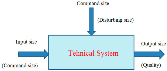
Figure 1.
General systemic description of a technical system.
Mathematically, the essential components that define safety in the exploitation of a system, under known working conditions (the availability, reliability, and maintenance of the system), i.e., without failures, are presented below.
Reliability, R(t), as a function of time (t—operation time, of variable size), represents the operation probability in a time range [0, t) [4] with predetermined parameters and without failures and has values between 0 and 1.
Practically, reliability is determined by calculation (established during product design [5,6]), followed by verification in the laboratory, and in system operation, the effective reliability is confirmed. For each product/element of the technical system, the reliability of each element resulting from series production can be determined [7], even with the start of the system’s operation, and so can its experimental reliability. Therefore, reliability is the main component of total quality control.
This paper’s theoretical notions refer only to dental bur active part wear, which is verified through a practical application. Thus, dental bur active part failure will be analyzed together with its wear, also experimentally [6,7,8].
The active part is the element of a dental bur that cannot be restored (which loses working capacity due to failure or wear [6,7,8]), i.e., it is not repairable but needs to be replaced/changed. The defect of the dental bur active part, in the studied case, represents a deviation from quality, and it assumes operation interruption in the set time range or the inability to function with the parameters imposed by the designer.
According to [8], defects are physical imperfections, material inconveniences, etc., that can appear during the execution phase, due to the material, the user, the equipment used, etc., and during operation, due to the working environment, wear, shocks, deformations, etc. Thus, by summing up the operation times of the system, the quantitative failures can be determined [6,9].
Dental burs are fine mechanics tools made of expensive materials and used for delicate operations from a technical point of view, so their rapid wear requires studies and research to extend their lifetime or even optimize their operation. This involves a detailed analysis of the working process based on the calculation of wear, which limits dental bur lifetime (durability and reliability) [9,10].
Understanding the advances in medical research in general [11,12,13,14] and in the field of dental applications in particular [10] is crucial to the appropriate interpretation of statistical results. Thus, the state of uncertainty and apparent chaos from nature can be transformed into measurable parameters, which is also applicable in dental practice, with the help of statistical tools. At the same time, understanding the meaning and actual extent of these instruments is essential and of great importance for researchers, practitioners, and users, who, based on evidence close to reality, constantly require up-to-date information and support for decision-making [15]. The various aspects of statistical analysis and results are reviewed, and their comprehension is then attempted based on common but not-yet-in-depth knowledge to obtain non-exhaustive, constructive, and realistic insights.
In the present case, the relationships for the analytical calculation of wear cannot be without certain coefficients that are obtained experimentally. At the same time, it is emphasized that to obtain analytical relations for the calculation of wear and tear, an obvious simplification and modeling of the influencing factors must be resorted to.
The results obtained experimentally in different fields (social, economic, industrial, etc.) and assuming the existence of normal conditions of interaction have highlighted the order of factors that can particularly influence the evolution of wear through the prism of wear speed during friction: the geometry and type of the friction pair, the lubricating environment, pressure, the surface condition and the local conditions of the friction surface, temperature, the nature of the materials of the friction pair, hardness, friction speed, etc. [16].
In the case of friction pairs with relatively simple geometry, relatively smooth surfaces, and variation in only two–three parameters, it is possible to obtain, by calculation, the influence on the speed or intensity of the wear. However, in the operation of a dental system (as with many other mechanical systems), the simultaneous intervention of several parameters makes analytical calculation difficult, especially since the phenomena at the level of the real area are random; therefore, a statistical calculation is required [16].
The mechanical processes of superficial interaction and friction give rise to the thermal processes of heat accumulation and transfer, which influence both the processes due to the action of the cooling/lubrication medium, chemical and tribochemical processes, and the processes of changing the phase and structure, with implications on the subsequent processes of superficial interaction and the final ones of dimensional change (wear).
The experimental analysis of a process/phenomenon must be validated by mathematical modeling, regardless of whether the mathematical model is theoretical, empirical, or mixed (theoretical–empirical) [17,18]. These models require vast experiences that allow for establishing the bonds/relationships between the input, output, and control parameters of the modeled process [19,20], and their validation is usually conducted through another set of experiences.
The working process of the dental burs is complex, similar to the friction and wear of materials, or even with their splintering. There are currently complex experimental studies being made on dental burs through advanced research methods [21,22], and interesting results are presented by Arsecularante et al., ref. [23].
Thus, very similarly to the fine machining process by splintering milling is the dental milling process. Within complex and very expensive research, these phenomena can be mathematically modeled based on the experimental results obtained. The accuracy and stability of the models/model are directly influenced by the large number of experimental data and parameters involved in the process. So, an integral part of the statistical analysis of experimental data now comprises statistical–mathematical models.
Therefore, the wear process of the dental burs’ active part is analyzed through the theoretical presentation of the methodology of analytical and practical statistical calculation for its wear and with appropriate explanations. Justification by the statistical calculation of dental burs’ active part wear will be conducted through experimental tests with practical applications regarding extending the lifetime and even optimizing operation, thereby providing new ideas for constructive solutions and establishing some criteria possible for the replacement of used dental burs.
2. Materials and Methods
The phenomenon of friction–wear stands out by its great complexity due to the multitude and interaction in the operation of all factors, both external (load, speed, environment, etc.) and internal (the material of the friction pairs with the respective structure and hardness, roughness, temperature, etc.). This perfectly objective situation, which is accentuated when moving from laboratory research on models to operational real conditions, explains to some extent the difficulties and the current state of wear calculation.
The interaction of the friction–wear processes is represented schematically in Figure 2, where you can see an image of the interdependence of the complex processes that take place on the friction surfaces. As a result of friction, a large part of the energy spent by this process is transformed into heat at the friction surface; this effect becomes decisive with the increase in the functional parameters (speed, load/pressure).
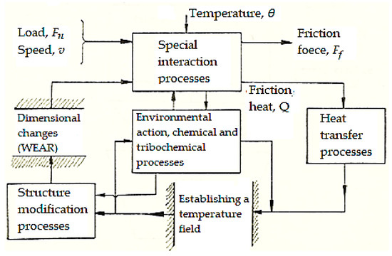
Figure 2.
Interaction diagram of friction–wear processes.
Thus, during operation, a friction pair can be considered as a system whose elements interact with each other, directly or indirectly. Input quantities/sizes of the system are the external parameters of the friction process (load Fn, speed v, working medium, temperature θ, etc.). Complex phenomena of superficial interaction take place on the friction surface, which in turn will produce displacement resistance (friction force Ff) and a quantity of heat Q (see Figure 2).
As a result of the heat accumulation and transfer processes, a temperature field will be established in the friction pair. The temperature field is of interest under the following aspects: the maximum temperature and its place of occurrence, the temperature gradient compared to the normals of the contact surfaces, and the spatial and temporal allure of the average temperature. For the good operation of the friction pair, the maximum temperature must not exceed the temperature of chemical stability, the critical temperature of the materials of the friction pair, and the ignition temperature of the various products in the system of which the friction pair is a part.
The direct effects of the temperature field lead to changes in the phase and structure of the materials on the friction surface and near it. Along with mechanical and metallurgical processes, chemical and tribochemical processes and the action of the environment (lubrication, cooling, etc.) intensify dimensional changes and therefore wear. On the other hand, the temperature field has a secondary reaction influence on the chemical and tribochemical processes and superficial interaction.
Damage to the surface and the games created (through wear) influence the initial interaction processes, with the cycle repeating, but with greater amplitude.
Therefore, mechanical processes of superficial interaction and friction, respectively, give rise to thermal processes of accumulation and heat transfer. These influence both the processes due to the action of the environment, chemical and tribochemical processes, and the processes of modifying the structure, with implications on the subsequent interaction processes, as well as the superficial and final dimensional changes (wear).
The elements that justify the statistical calculation of wear are presented in detail in refs. [6,9,10,24] and can be synthesized in two main directions:
- -
- Statistical nature of the friction–wear process, namely the following: the random mode of production of real area contacts, the formation of wear particles, the variation in the surface structure and condition, the variation in external parameters, action mode of the lubricants and additives, etc.);
- -
- Analytical calculation relationships include factors that can be constant and experimentally determined coefficients, but they cannot separate the influence of the weight of the respective factors and cannot cover all types of wear that contribute to surface degradation.
The statistical calculation of wear has the advantage that the relationships obtained by statistical means—regression relationships—are relatively easy to obtain, starting from data and experimental results, which include the interaction of all factors [9,10].
However, knowing the error, with such relations a considerably larger volume of information can be obtained than that entered for their determination.
To be able to apply certain quantitative methods for extracting the desired information, it must be possible to find a (statistical) model of the studied phenomenon that incorporates its essential characteristics as realistically as possible. At the same time, the (statistical) model must not be too complicated for analytical handling [6,8]. Also, it is necessary that the phenomenon (process) studied statistically can be mathematically formalized conveniently. The solution to this problem (of finding the statistical–mathematical model) was the concept of a random variable whose value is a number determined by the event resulting from an experiment.
It is mentioned that for the experimental tests, only one type of conical–cylindrical dental bur (presented below in Section 3.2 and frequently used in practice) was used as a sample, in the number of 16 pieces. The 16 dental burs were divided into 4 groups of 4 pieces, with each group being tested at a different rotation speed (7000, 12,000, 20,000, and 35,000 rpm). Thus, for each of the chosen rotation speeds of 7000, 12,000, 20,000, and 35,000 rpm and this dental bur type (conical–cylindrical), the wear was evaluated after 4 h of operation (from hour to hour, at each rotation speed).
The wear was evaluated by mass loss of the active part of each dental bur and weighing. Weighing was conducted before and after the operation for each of the 16 tested dental burs. For weighing, an analytical balance was used with a capacity of up to 320 g and a precision of 0.0001 g. After each hour of operation and at each rotation speed, the dental bur was replaced with another one, and the test was repeated 5 times (under the same conditions, for each dental bur).
3. Results and Discussions
3.1. Theoretical Aspects
The distribution law establishes the correspondence between the random values, xi, and the respective probabilities, pi, using an analytical relationship as follows: P(X = xi) = P(xi) = pi called the probability of failure or failure function, F(x), which can be empirical or theoretical. If the phenomenon/process probability, P(X = xi), is obtained after the experience based on the statistical observation data, then the statistical probability is a relative frequency, and the distribution is empirical. The failure function, F(x), is the most representative characteristic of a random variable and is defined as the phenomenon/process probability, so that the random variable, X < x, is given/known:
If X follows a continuous statistical distribution, F(x) has the form as follows:
where f(x) is the frequency function (probability distribution density), which is the derivative of the function, F(x), and R(x) is the reliability function. The plot of the function, f(x), is illustrated in Figure 3.
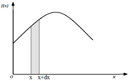
Figure 3.
Variation plot of the function, f(x), for continuous functions.
The size value, f(x)dx, represents the probability that the variable, x, belongs to the elementary interval, dx. The function plot, F(x), from Figure 4 looks like the following:
that is, the area bounded by the function curve, f(x), and the abscissa axis are equal to unity.
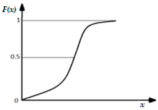
Figure 4.
Distribution function continuous, F(x).
When studying a quality characteristic, the experimenter has at their disposal observation data obtained by measurements of durability. This durability is a random variable. Even if its distribution is not known, certain indicators and certain measures [7] of the trend of the considered variable are necessary.
An experimental distribution (obtained through observations) that is, respectively, empirical shows a variation tendency with two aspects for any characteristic of the population: localization around a certain value (position) and, respectively, variation (scattering), as shown in Figure 5.
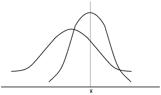
Figure 5.
Representation of distribution functions for phenomena/processes with different scatters.
It is noted that the distribution can be symmetrical or asymmetrical about the location area. The statistical indicators with which a quantitative analysis can be performed to compare trends in location and variation (dispersion) are as follows:
- (a)
- Location indicators—these indicate the value where the real data of the phenomenon/process tends to cluster, and the main indicator is the average [25] (with arithmetic average being the most important), M(X), and
- (b)
- Variation indicators—these represent the deviation of the values, x, from their arithmetic mean and include the following:
- -
- Dispersion, D(X) or σ2 (σ = )—this represents the square mean deviation, and if it is defined in ratio with the mean value, , the mathematical relationship is as follows:The average squared deviation, σ, calculated is a “guarantee” of the accuracy of the determinations only if there are at least three values [8]. The calculation is made only if the distribution is normal (Gaussian) or almost Gaussian. In addition, the value of σ allows conclusions to be drawn only if these come from at least 30 values simultaneously.
- -
- Quartile of the random variable, Xα, defined as the equation root:and this is another reliability indicator, and α is defined as a percentile.F(Xα) = α,
This indicator expresses the time at which a system or its component works with a certain probability (1 − F(x)).
The collected (experimental) data on the values of the investigated characteristic are presented as a disordered table, and by ascending ordering them, the statistical string (series) is obtained. Data grouping is conducted on intervals, the size of which is generally taken to be equal, except for extreme intervals, at which the values can be different. The number of intervals can be established with the relationship [7,26,27]:
where Z is the record data total number.
n = 1 + 3.322 lg Z,
The size (amplitude) of the interval (class) is as follows:
where xmax and xmin are the maximum and minimum values of the data string [7,8,27,28].
During the execution of tests and the collection of experimental data, values appear that are substantially different in size from the other values of the respective statistical series (they are much smaller or much larger). Because of this, it is natural to suspect these data are not from the statistical string/series. These are due to specific random influencing factors, measurement errors, and data recording mistakes, or coming from a phenomenon/process other than the one under study. There is no known criterion for the instant recognition of the presence of outliers [8], which differ from the other values of the statistical series.
There is a rich palette of statistical criteria to identify the presence of outliers, but to minimize them, it is necessary to reach a state of stability. This is possible when the two parameters of the selection are known: the mean, , and the dispersion, D(X), respectively, as well as the mean square deviation, σ, of the data.
For the analysis of a parameter, it can be estimated pointwise (as an isolated value or as one confidence interval), if an interval is established to include with a probability, P, the true value of the estimated parameter. Therefore, the probability value, P, implies a certain interval, (x1, x2), according to the relationship:
and to which the respective parameter belongs.
It is mentioned that there is a “risk” or the probability that the true value will fall outside the considered confidence interval.
Depending on how the risk is placed on the confidence interval, it can be as follows:
- -
- Confidence interval with bilateral risk (symmetric or asymmetric risk is placed with equal values (α/2) on either side of the extreme values of the interval, Figure 6).
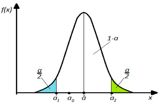 Figure 6. Interval with bilateral symmetric risk. Note: a0—the true value of the estimated parameter; a—the probability of the analyzed parameter; (a1, a2)—the confidence interval.
Symmetric confidence intervals (see Figure 6) are widely used in measurement techniques where the deviations of quantities in one direction or another have the same importance, and the confidence interval with asymmetric bilateral risk (Figure 7) is frequently encountered in industrial applications, technology, design, etc.
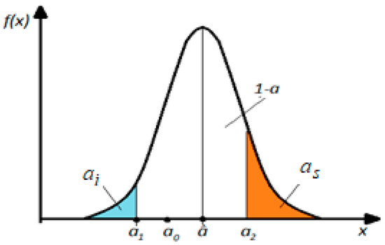
Figure 7.
Interval with bilateral asymmetric risk. Note: a0—the true value of the estimated parameter; a—the probability of the analyzed parameter; (a1, a2)—the confidence interval.
Confidence limits are determined only if the amount of information is large enough to be able to characterize the multitude of products of the same type. The determined minimum and maximum values form a range of values in which any, and σ, must fall into any other sub-crowd of products tried under other conditions, a sub-crowd which is part of the crowd given.
The surface, a, (under the curve of the f(x) function, see Figure 6) guarantees the probability of including the indicators corresponding to the respective range of values.
3.2. Practical Application
A practical/applicative example will be presented next, for the dental bur of the type in Figure 8, where x = t is the time of good operation of the dental bur, so xi = ti; X = td is also the specified limit of the duration of good operation, or the operation time until the first system failure (here the dental bur active part).
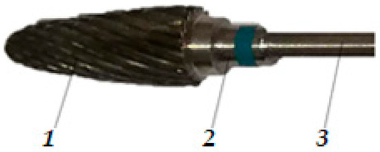
Figure 8.
Conical–cylindrical dental bur: 1—dental bur active part; 2—dental bur neck; 3—dental bur foot.
These dental burs are made of a metallic mixture in which tungsten carbide (WC) dominates together with other carbides of Cr, Mn, Fe, etc., with the medium graining on the active part. They are used for processing Co-Cr alloys, as well as metals, both semi-precious and precious metals. Such a dental bur is provided with a blue ring for identification, marked on position 2 in Figure 8, and works at speeds up to 35,000 rpm.
At the same time, on the active part of the dental burs there are cutting lamellae wounds, arranged equidistantly and oriented to the right, with a pitch of about 0.65 mm, seating angle of 47.740 degrees, sharpening angle of 61.480 degrees, clearance angle of 9.900 degrees, maximum diameter of 6.20 mm, average diameter of 5.40 mm, length of the active part of 14.50 mm, total length of 52.75 mm, and average mass of 4.701 g.
The conventional lifetime (conventional durability), tμ, of the dental bur active part in Figure 8 was estimated using the formula for calculating the working time (optimal functioning), given the relationship [9,29] as follows:
where μ is a fraction from the dental bur active part total mass, established conventionally and lost during the work/functioning process; ω is the dental bur angular speed; d is the model parameter (d = 3.5 × 10⁻⁵) dependent on the lost mass through the dental bur active part wear and tested on the angular space (circular friction length), φ = ω·t.
The critical fraction of material, μ, which is lost in the work process from the dental bur active part was established, starting from about 65% of the approximate circular crown mass, determined experimentally through the active part total wear (as mass lost). Then, by weighing and calculating the difference compared to the dental bur specimen (Figure 9) the value of 0.408 g was obtained.
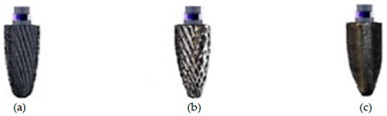
Figure 9.
Methodology of establishing the circular crown mass of the dental bur active part: (a) specimen dental bur, after 1 h of operation; (b) worn dental bur after 4 h of operation; (c) dental bur with the circular crown of the active part, completely worn.
It is mentioned that milling wear is estimated by the reduction in the tool diameter (bur) on a certain contact width [30] and is consistent with the weight loss, as a result of wear, in the dental bur work process. Thus, Table 1 presents the dental bur characteristics taken as a specimen.

Table 1.
Mass and dimensions of the dental bur specimen.
The lifetime results (calculated with relation (10) and presented as average values) for the dental burs of the same type, in number of 16, tested in the laboratory (see Figure 7), for 4 h and at 4 rotation speeds are those presented in Table 2, the column “Lifetime (Duration) calculated, hours”.
Table 2.
Average lifetime calculated for the dental bur active part, researched experimentally.
The wear was evaluated by the mass loss of the dental bur active part by weighing, during 4 h of operation, at each of the rotation speeds of 7000, 12,000, 20,000, and 35,000 rpm and presented graphically in Figure 10.
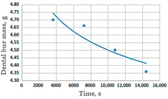
Figure 10.
Variation in time of the lost mass in the dental bur work process. Note: the points in the graph represent the average value of the cumulative mass loss in time for the 4 rotation speeds and 5 repetitions considered in the experiment.
Initially, the dental bur mass was 4701 g, and after 4 h of operation and at four different rotation speeds, it reached the value of 4360 g (see Figure 10).
Given the experimental results, respectively, by the user consultation of dental burs (doctors and dental technicians) with those who use/consume them a lot, the following was found:
- -
- Failure probability in the work process of the dental bur active part is very low until a minimum time, t1, and then it grows rapidly up to a maximum time, t2, when practically, in general, no bur is usable anymore;
- -
- Time range, t2–t1, when the dental bur active part is taken out of operation, is due to the small differences between parameters (with masses, angles, etc., being a little different) of the same active parts.
Finally, these differences influence the lifetime, a thing observable from the durability calculation (see Table 2). The range [t1, t2] of increase in the failure probability is greater by how much the differences between active parts from the same set, or type, are bigger. Based on these findings, for the operation of dental burs without defects, the following reliability function is proposed [31,32]:
where t2 is the maximum time after which the dental bur active part of the same type and brand was damaged, in the experiment time, and m is an exponent parameter, chosen so that the time, t1, at which failure probability (reliability), R(t), begins to grow exponentially can be estimated as best as possible.
A satisfactory estimate is obtained for m = 0.75, in this case, and the reliability function variation, R(t), in time (according to the relationship (11)) is represented graphically in Figure 11. Thus, for dental burs of the same type, whose lifetime at the rotation speed of 7000 rpm is 20,526 h after 1 operating hour, 19,265 h after 2 h of operation, 21,573 h after 3 h of operation, and 20,368 after 4 h of operation, respectively, the average value of the lifetime is 20,433 h and is presented in Table 2. It turns out that the estimated minim and maxim times (according to the above) are t1 = 19,265 h and t2 = 21,573 h, respectively, obtained by calculation from the experimental determinations.
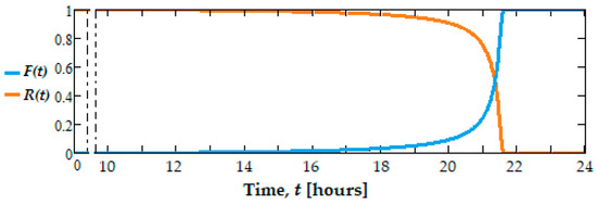
Figure 11.
Plots of reliability functions, (R(t) and failure, F(t), for the tested dental bur active parts.
In Figure 11, the failure function plot, F(t), is also shown, and in Figure 12 the frequency function plot, f(t), which corresponds to the reliability function, R(t), from relation (11).
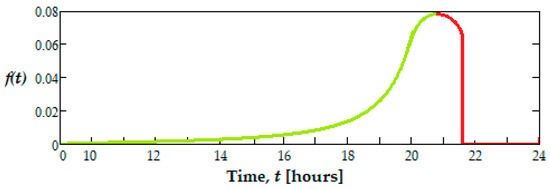
Figure 12.
Frequency function plot, f(t), for the tested dental burs.
Analyzing Figure 10 and Figure 11, it can be seen that R(t) is monotonically decreasing, and instead F(t) is increasing. These functions take values in the range [0, 1] because when t → ∞, R(t) = 0, F(t) = 1 and when t → 0, R(0) = 1, F(0) = 0, f(t) verifies the relationship .
The dental burs’ reliability can also be specified with the help of the numerical values of the indicators attached to the operating time, t (variable), until the first failure. These indicators (presented above) are M(t), D(t), σ, and tα, etc.
The values, M(t), of the operation time without failure are determined with relation (4) and presented in Table 2. By integration of the function, M(t), t = 20,433 h was obtained in the working conditions at the rotation speed of 7000 rpm.
When the system (the dental bur active part) is without reconditioning, then M(t) represents the average time without system failure, until the first failure. M(t) of the system, i.e., the average value of t, can be expressed either by function R(t) or function f(t) (see relation (4)).
The variation in the random variable, t, or the distribution variation, D2(t), is defined by relation (5) and is obtained through D2(t) = 2.562 h, and the mean square deviation, σ, of t is the indicator that can often be used instead of D2(t) and results from 1.600 h.
D2(t) and σ show the degree of uniformity of system/product performance (here, dental burs of the same type) from the point of view of reliability, by their values. If the technological process of manufacturing the system/product is well established, then the D2(t) and σ values are relatively small and show us the degree of uniformity of the set of tested dental burs, as in the present case.
The last important reliability indicator considered is the operating time quartile, tα, defined as the root of the equation:
and what results from equation/relation (6) and α with values from 0.01, …, 0.99 is defined as a percentile.
At a rotation speed of 7000 rpm and α = 0.99, tα = 21,502 h was obtained. In the reliability theory, the value his this tα is interpreted as a guaranteed time, i.e., the period when the defective elements proportion in a certain system/group does not exceed the value, α pre-set initially established [4]. The value of tα = 21,502 h is very close to t2 = 21,573 h, calculated analytically, which justifies the correlation between the theoretical and experimental results.
As stated above, the first data collected regarding the values of the investigated parameter (the lost mass by the dental bur active part) is presented as a disordered mass, and by ordering (ascending) of the experimental data, the statistical series is obtained.
The grouping of the data is conducted on grouping intervals, whose number, n, calculated with relation (7) is n = 5 (it must be an integer and was considered to be Z = 16 tested dental burs) and whose size is generally taken to be equal, except for the extreme intervals, when it can use different values. The size (amplitude) of the interval is determined based on relation (8) and is A = (1.4 − 0.5)/5 = 0.18.
Another important role in the reliability theory also has the function, h(t) = f(t)/R(t), R(t) ≠ 0, that measures the intensity (rate) of failure (the instantaneous risk of failure), or the hazard of a system/component product, defined as the failure rate limit in the interval [t, t + Δt], Δt > 0 being very small [4], whose variation is presented in Figure 13, which was used.
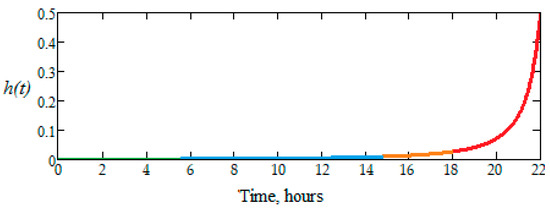
Figure 13.
Instantaneous risk (failure) function plot, h(t), for the investigated dental burs.
It can be seen that the failure risk rate is around 10%, for 20 h, and increases approximately exponentially in the 21st hour of operation. This means that the dental bur active part is taken out of operation after 20 h of operation, and it is normal that it be replaced.
The evolution of function h(t) shows that there is no failure risk, in the range t Є (0, 14) hours, with the variation being linear, and with a very small slope. In the range t Є (14, 18), the wear phenomenon becomes visible because h(t) has a variation after a fast-growing curve, and therefore the risk of failure increases. Then, in the range t Є (18, 21) hours, the failure risk becomes inevitable, when the plot of h(t) suddenly increases after an exponential curve.
Therefore, it is confirmed that the experimental results correlate with the analytical ones for the researched dental burs, i.e., they can work without major risk of failure for up to 18 h. At the same time, this proves the closeness between the hours determined analytically based on the experimental results to those of operation without a major failure.
On the other hand, when measuring by the weighing of mass lost through wear by the dental bur active part and presented in Table 2 as obtained different random values, each value has several repetitions, so it has a frequency of its own. These values are located in an interval with two limit values (lower and upper).
The value distribution between the two limits of the range can vary (with their frequency) after a distribution law. It is mentioned that the variation range of a property/characteristic/parameter reflects the quality level of a product of industrial manufacturing.
The lost mass values through effective wear (random variable) are distributed after the normal (Gaussian) distribution law because factors that determine their dispersion through wear are of the same order, accidental and independent, in large numbers and must be less than a given value that corresponds to a probability, p, i.e., of reliability, R(t)).
The normal distribution or Gaussian one represents the frequency function or probability distribution density, f(x), which is closest to a normal distribution function of the shape:
whose variation over time is shown in Figure 14.
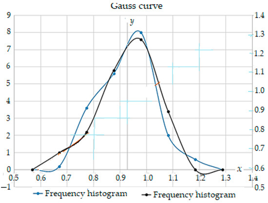
Figure 14.
Probability density plot for the Gaussian (normal) distribution law.
It is observed on the probability density function curves that there are two inflection points of abscissas 0.88 and 1.08, where the area bordered by these abscissas and curves represents about 58.33% of the entire surface.
This proves that the values of mass lost by wear of the dental bur active part are the most distributed.
The curves present a maximum of approximately y = 5.03 at x = 0.95 (blue curve) and y = 4.98 for the same x = 0.95 (curve that is black), with the reliability obtained being approximately 97.42% of the entire area (i.e., limited by the curves and the abscissa axis, in the range (0.67, 1.18)—the confidence range), so the reliability is excellent, and the intervals (−∞, 0.67) and (1.18, +∞) can be practically neglected.
Thus, the scattering/confidence range is (0.67, 1.18), with limit deviations of ±0.25 compared to the values distribution center (cluster), and the critical range is (−∞, 0.67) U (1.18, +∞). Therefore, the lost mass values through wear have a Gaussian (normal) distribution, and the function, f(x), is a normal distribution function or the probability distribution density (the blue and black curves from Figure 14).
4. Conclusions
- -
- The phenomenon of friction–wear is complex, due to the multitude and interaction in the operation of all factors, both external (load, speed, environment, etc.) and internal (the material of the friction pair with the respective structure and hardness, roughness, temperature, etc.). It is a perfectly objective situation, which is accentuated when moving from laboratory research on models to operational real conditions, explaining to some extent the difficulties and the current state of wear calculation.
- -
- The wear statistical calculation starts from the real situation reflected by experimental data as the basis for the analytical calculation relations (regression relations), given the interaction of all influencing factors. It is justified, even from the statistical nature of the friction–wear process.
- -
- It is necessary to find a (statistical–mathematical) model for the studied phenomenon/process (wear of the dental bur active part) in view of the quantitative extract of the desired information. At the same time, it must not be too complicated for analytical handling but must incorporate its essential characteristics as realistically as possible.
- -
- The solution to this problem is the concept of a random variable (here mass loss of the active part of the dental bur)—a quantity determined by the event resulting from the performance of an experiment (establishing the operating time without failures, in this case). To compare random variables, the distribution function, F(x), is used.
- -
- When the values come from a normal distribution, some of the main statistical parameters, average, dispersion, mean square deviation, etc., are determined and checked. If these checks do not lead to favorable conclusions regarding the normality of the data distribution, the measurement data from the statistical series will be checked more thoroughly.
- -
- The results showed that the investigated dental burs may operate without failure major risk until 18 h, very close to those determined to be experimental, which validates the correlation between analytical calculation and the experimental test results. Practically, based on the results presented in this paper, it was found that dental burs during the milling operation can easily become decommissioned, resulting in mass loss, and in the first 18 h of work, they operate with high efficiency.
- -
- Over this number of operating hours, to ensure high standards of material processing, the dental burs should be replaced with new ones. Additionally, the methodology applied in this paper showed that it is possible to increase the lifetime by approximately 10% and it allows for investigation of the possibilities of improving or optimizing the working regimes of dental burs.
- -
- The researched parameter of the analyzed dental burs was the mass lost through wear, determined by weighing, taking different random values, between two limits, with each value repeating itself several times (having its frequency), and their scattering can be represented through a distribution law.
- -
- Most experimental data of the mass lost by the wear of the dental bur active part are very close to the Gaussian normal distribution, and the probability density (frequency function) is a normal distribution function, so it is Gaussian.
- -
- In perspective, it is envisaged to expand the analysis of wear behavior by statistical calculation, based on experimental data, and to other types of dental burs, also considering other parameters.
Funding
This research received no external funding.
Institutional Review Board Statement
Not applicable.
Informed Consent Statement
Not applicable.
Data Availability Statement
The original contributions presented in the study are included in the article, further inquiries can be directed to the corresponding author.
Conflicts of Interest
The author declares no conflicts of interest.
References
- Kapur, K.; Feng, Q. Statistical Methods for Product and Process Improvement. In Springer Handbook of Engineering Statistics; Pham, H., Ed.; Springer Handbooks; Springer: London, UK, 2006. [Google Scholar] [CrossRef]
- Available online: http://dexonline.net (accessed on 30 September 2023).
- Liu, T.; Yu, J.; Wang, H.; Li, H.; Zhou, B. Modified Method for Determination of Wear Coefficient of Reciprocating Sliding Wear and Experimental Comparative Study. Mar. Sci. Eng. 2022, 10, 1014. [Google Scholar] [CrossRef]
- Burlacu, G.; Danet, N.; Bandrabur, C.; Duminica, T. Reliability, Maintainability and Availability of Technical Systems; Matrimax Publishing House: Bucharest, Romania, 2005; ISBN 973-685-891-X. (In Romanian) [Google Scholar]
- Vodă, V.; Isaic-Maniu, A.L.; Bârsan-Pipu, N. Failure: Statistical Models with Applications; Economic Publishing House: Bucharest, Romania, 1999; ISBN 973-590-179-X. (In Romanian) [Google Scholar]
- Pavelescu, D. Tribotehnica; Technical Publishing House: Bucharest, Romania, 1983. (In Romanian) [Google Scholar]
- Laurent, L.; Pillet, M. Conformity and statistical tolerancing. Int. J. Metrol. Qual. Eng. 2018, 9, 1–8. [Google Scholar] [CrossRef][Green Version]
- Văleanu, I.; Hâncu, M. Elements of General Statistics. Ph.D. Thesis, Litera Publishing House, Bucharest, Romania, 1990. (In Romanian). [Google Scholar]
- Ilie, F.; Saracin, I.A. Establishing the Durability and Reliability of a Dental Bur Based on the Wear. Materials 2023, 16, 4660. [Google Scholar] [CrossRef] [PubMed]
- Ilie, F.; Saracin, I.A.; Voicu, G. Study of Wear Phenomenon of a Dental Milling Cutter by Statistical–Mathematical Modeling Based on the Experimental Results. Materials 2022, 15, 1903. [Google Scholar] [CrossRef] [PubMed]
- Garmendia, J.L.; Maroto Monserrat, F. Interpretation of statistical results. Med. Intensiva. 2018, 42, 370–379. [Google Scholar] [CrossRef]
- Greenwood, D.C.; Freeman, J.V. How to spot a statistical problem: Advice for a non-statistical reviewer. BMC Med. 2015, 13, 270. [Google Scholar] [CrossRef] [PubMed]
- Altman, D.G. Statistical reviewing for medical journals. Stat. Med. 1998, 17, 2661–2674. [Google Scholar] [CrossRef]
- Wiedermann, C.J. Ethical publishing in intensive care medicine: A narrative review. World, J. Crit. Care Med. 2016, 5, 171–179. [Google Scholar] [CrossRef] [PubMed][Green Version]
- Cole, G.D.; Nowbar, A.N.; Mielewczik, M.; Shun-Shin, M.J.; Francis, D.P. Frequency of discrepancies in retracted clinical trial reports versus unretracted reports: Blinded case–control study. BMJ 2015, 351, h4708. [Google Scholar] [CrossRef] [PubMed][Green Version]
- Pavelescu, D.; Musat, M.; Tudor, A. Tribologie; Didactic and Pedagogical Publishing House: Bucharest, Romania, 1977. (In Romanian) [Google Scholar]
- Qehaja, N.; Abdullahu, F. Mathematical Modelling of the Influence of Cutting Parameters and Tool Geometry on Surface Roughness During Drilling Process. Sci. Proc. XIV Int. Congr. Mach. Technol. Mater. 2017, 6, 439–442. [Google Scholar]
- Rehman, G.U.I.; Jaffery, S.H.I.; Khan, M.; Ali, L.; Khan, A.; Butt, S.I. Analysis of Bur Formation in Low Speed Micro-milling of Titanium Alloy (Ti-6AI-4V). Mech. Sci. 2018, 9, 231–243. [Google Scholar] [CrossRef]
- Chetan Narasimhulu, A.; Ghosh, S.; Parchuri, V.R. Study of Tool Wear Mechanisms and Mathematical Modeling of Flank Wear During Machining of Ti Alloy (Ti6AI4V). J. Inst. Eng. 2014, 96, 279–285. [Google Scholar] [CrossRef]
- Chinchanikar, S.; Choudhury, S.-K. Characteristic of wear, force and their inter-relationship: In-process monitoring of tool within different phases of the tool life. Procedia Mater. Sci. 2014, 5, 1424–1433. [Google Scholar] [CrossRef]
- Jaffery, S.H.I.; Khan, M.; Ali, L.; Mativenga, P.T. Statistical analysis of process parameters in micromachining of Ti-6Al-4V alloy. Proc. Inst. Mech. Eng. Part B J. Eng. Manuf. 2016, 230, 1017–1034. [Google Scholar] [CrossRef]
- Cardei, P.; Saracin, A.; Saracin, I. A classical mathematical model applied for the study of the phenomenon of wear od dental mills. Preprint RG 2020. [Google Scholar] [CrossRef]
- Arsecularatne, J.-A.; Chung, N.-R.; Hoffman, M. An in vitro study of the wear behaviour of dental composites. Biosurface Biotribology 2016, 2, 102–113. [Google Scholar] [CrossRef]
- Blau, P.J. Tribosystem Analysis: A Practical Approach to the Diagnosis of Wear Problems, 1st ed.; CRC Press: Boca Raton, FL, USA; Taylor & Francis Group: Abingdon, UK, 2016. [Google Scholar] [CrossRef]
- Birolini, A. Chapter 7: Statistical Quality Control and Reliability Tests. In Reliability Engineering; Springer: Berlin/Heidelberg, Germany, 2017. [Google Scholar] [CrossRef]
- Queiroz, T.; Monteiro, C.; Carvalho, L.; Francois, K. Interpretation of Statically Data: The Importance of Affective Expressions. Stat. Educ. Res. J. 2017, 16, 163–180. [Google Scholar] [CrossRef]
- Li, J. Application of Statistical Process Control in Engineering Quality Management. IOP Conf. Ser. Earth Environ. Sci. 2021, 831, 012073. [Google Scholar] [CrossRef]
- Tudor, A.; Gh, P.; Muntean, C.; Motoiu, R. Durability and Reliability of Mechanical Transmissions; Technical Publishing House: Bucharest, Romania, 1988. (In Romanian) [Google Scholar]
- Saracin, I.A. Studies and Research on the Durability and Realiability of Dental Milling Cutters. Ph.D. Thesis, Politehnica University of Bucharest, Bucharest, Romania, 2021. (In Romanian). [Google Scholar]
- Cho, J.-H.; Yoon, H.-I.; Han, J.-S.; Kim, D.-J. Trueness of the Inner Surface of Monolithic Crowns Fabricated by Milling of a Fully Sintered (Y, Nb)-TZP Block in Chairside CAD-CAM System for Single-visit Dentistry. Materials 2019, 12, 3253. [Google Scholar] [CrossRef] [PubMed]
- Fry, R.; McManus, S. Smooth Bump Functions and Geometry of Banach Spaces, A Brief Survey. Expo. Math. 2002, 20, 143–183. [Google Scholar] [CrossRef]
- Available online: https://mathworld.wolfram.com/BumpFunction.html (accessed on 12 October 2023).


Disclaimer/Publisher’s Note: The statements, opinions and data contained in all publications are solely those of the individual author(s) and contributor(s) and not of MDPI and/or the editor(s). MDPI and/or the editor(s) disclaim responsibility for any injury to people or property resulting from any ideas, methods, instructions or products referred to in the content. |
© 2024 by the author. Licensee MDPI, Basel, Switzerland. This article is an open access article distributed under the terms and conditions of the Creative Commons Attribution (CC BY) license (https://creativecommons.org/licenses/by/4.0/).