Abstract
The current literature mainly uses hub capacity or transport route selection to manage the congestion of emergency multimodal transport and pays less attention to transshipment scheduling. This paper proposes an integrated optimization problem of transport routes and transshipment sequences (ITRTSP) and constructs a hybrid flow shop scheduling model to describe it. Based on this model, a recursive method is proposed to calculate the minimum waiting times that cargoes consume in queues at hubs, given the transport routes and transshipment sequences. Furthermore, a memetic algorithm is designed with route selection as the outer layer and transshipment sequence selection as the inner layer for solving ITRTSP. Compared with existing achievements, the model and algorithms can quantify the dependency between transshipment sequence selection and emergency transport time in multimodal transport network settings. The model and algorithms are applied to solve some real-scale examples and compared with the first-come-first-served (FCFS) rule commonly used in the current literature. The results indicate that the makespan is reduced by up to approximately 4.2%, saving 33.68 h. These findings demonstrate that even with given hub capacities and transport routes, congestion can still be managed and the schedule optimized through transshipment scheduling, further improving emergency transport efficiency.
1. Introduction
In the past decades, rail transport has played an important role in responding to major emergencies such as armed conflicts, terrorist attacks, and natural disasters [1]. Numerous practices [2,3,4] have shown that using railways for cross-regional and long-distance land transport can improve emergency efficiency and shorten response time. However, due to the constraints of the rail infrastructure, railways cannot directly provide “door-to-door” services. Generally, the transport between the rail transshipment hubs (after this referred to as hubs) and origins or destinations requires assistance from road systems [5]. In other words, if railways are used for emergency transport, the combined transport of roads and rails will usually become an inevitable choice. Given this, it is of great practical value to study road–rail multimodal transport optimization from the emergency perspective [6].
Numerous studies suggest minimizing response time is the top priority in emergency transport decisions [7]. Generally, when considering the schedule of road–rail multimodal transport tasks, congestion at hubs (after this referred to as congestion) is an important issue that cannot be ignored. Unlike road transport, road–rail multimodal transport requires transshipment operations at hubs (i.e., transshipping cargo from trucks to trains, or vice versa). Due to the limited transshipment efficiency, queuing is usually unavoidable when the loading or unloading efficiency does not match the arrival rate [8]. In large-scale emergency transport, it is common for temporary freight demand beyond the capacity of the transport network [9]. If congestion cannot be effectively controlled when developing road–rail multimodal transport schemes, the waiting time for cargo to be transshipped at hubs (after this referred to as the waiting time) would be prolonged and negatively affect the overall schedule for emergency transport.
In recent years, congestion management has become one of the hotspots in multimodal transport research. Existing literature [5,10] mainly explores solutions from strategic and operational perspectives. From a strategic perspective, the supply of hub resources determines the transshipment efficiency of multimodal transport systems. Some studies [11,12,13] control congestion by adjusting the number and location of hubs or equipping hubs with appropriate transshipment facilities. Optimizing multimodal transport schedules becomes another natural choice when demand and hub capacity are known. At present, adjusting the arrival rate is the primary means at the operational level. For example, some studies [14,15] provide the traffic flow limits of hubs, while others [16,17,18,19] formulate the transshipment time or cost as a function of cargo arrival rate and hub transshipment efficiency. Studies on emergency-related multimodal transport [20,21,22] also follow these ideas. For example, Ref. [20] considered the damage on routes and hubs to propose an integrated approach for solving the post-disaster multimodal transport network recovery and relief supplies transport problem. To manage congestion, both perspectives were considered: Optimize the repair plan for damaged hubs first to further determine the transshipment efficiency of the hubs during the repair period and then adjust the arrival rate under the given transshipment efficiency. However, due to the lack of specific descriptions of transshipment operations, the above studies do not focus on the impact of the transshipment scheduling details on the waiting time.
In fact, efficient transshipment scheduling can save the time that cargoes spend at hubs. Many multimodal transport studies have focused on this goal. For example, certain studies [23,24] have optimized crane scheduling within hubs to minimize vehicle waiting time; other studies [25,26] have improved yard storage strategies to reduce non-operational time, thereby enhancing transshipment efficiency; Gao, Y. et al. [27,28] focus on traffic management at hubs and stowage planning to improve transshipment efficiency; and furthermore, Kizilay et al. [29] have integrated crane scheduling, yard management, and internal traffic planning to develop more comprehensive hub operation scheduling solutions. However, these studies primarily focus on optimizing the scheduling at an individual hub rather than across all hubs at the level of the entire multimodal transport network to improve overall operational efficiency.
Claudia et al. [5] argued that the researchers need to pay attention to the impact of transshipment plans on congestion under the circumstances of road–rail multimodal transport, e.g., loading and unloading operations, traffic management at transshipment terminals coordinated with operation scheduling, and yard management problems. Some studies [8,10,30,31,32,33] introduced queuing models to describe the process of transshipping operations. First, the first-come-first-served (FCFS) rule is used for transshipment sequencing. Then, the arrival of cargo at each hub is modeled as a Markovian queue, and based on Little’s law to estimate the average waiting time. However, such methods have limitations in solving emergency multimodal transport problems. Since using average waiting time substitutes for actual waiting times, such methods cannot accurately estimate the impact of transshipment operations on the schedule of multimodal transport. More importantly, as only the FCFS rule was considered, these achievements do not fully demonstrate the role of transshipment sequence selection in congestion management.
When considering time goals, the FCFS rule may not be the optimal sequencing rule for managing congestion in multimodal transport systems. For example, to shorten the waiting time for hazmat at the hub, Assadipour et al. [32] introduced a hazmat priority rule (i.e., hazmat containers have priority over regular containers) besides the FCFS rule to optimize the transshipment sequence. This study enlightens that congestion can also be managed by transshipment sequence selection besides hub capacity and transport route, further optimizing the road–rail multimodal transport schedule. Given the significant value of shortening response times in emergencies, it is necessary to develop an analytical method to explore the systematic effects of transshipment sequence selection on the road–rail multimodal transport schedule. This paper focuses on the dependency between transshipment sequence selection and waiting time, and proposes an integrated optimization problem of transport routes and transshipment sequences (after this referred to as ITRTSP, see Section 2.1) at the operational level, comprising two sub-problems: (1) Allocating hubs for all cargoes to determine transport routes; (2) Selecting transshipment sequences for cargoes at the same hub.
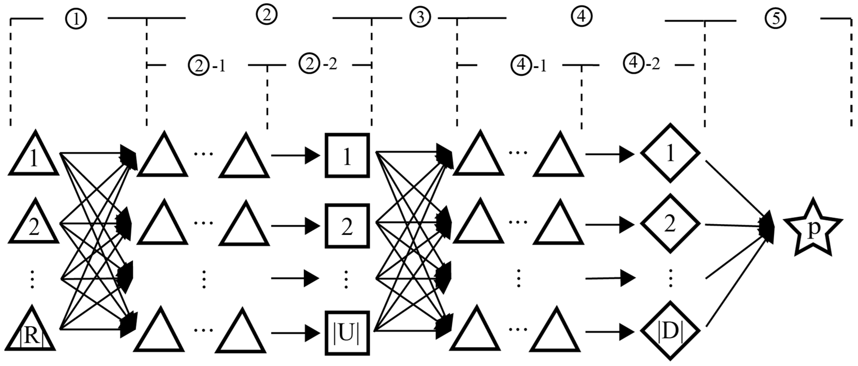
Due to the further consideration of transshipment sequence selection based on hub allocation, ITRTSP is highly similar to the hybrid flow shop scheduling problem (HFSP) [34] in objectives, variables, and constraints. Usually, the road–rail multimodal transport process in emergencies (see Figure 1 for the meanings of symbols in Section 2.1) can be divided into five fixed sequential operations: ① road transport from an origin to a hub responsible for loading onto trains (referred to as an upstream station); ② transshipment at the upstream station, including queuing (operation ②-1) and loading (operation ②-2); ③ rail transport to a hub responsible for unloading from trains (referred to as a downstream station); ④ transshipment at the downstream station, including queuing (operation ④-1) and unloading (operation ④-2); ⑤ road transport to a destination. From Figure 1, it can be seen that if all cargoes are treated as jobs that need to be processed (transshipped), and the upstream and downstream stations are treated as multiple parallel machines with limited loading and unloading efficiency, then ITRTSP can be modeled as a two-stage HFSP with transport constraints [35].

Figure 1.
The operation process of road–rail multimodal transport.
Compared to the achievements based on queuing theory, transforming ITRTSP into HFSP has two main advantages. Firstly, models of HFSP can quantitatively describe the dependency between transshipment sequence and waiting time. Secondly, solution methods of HFSP can calculate the minimum waiting time (not the average waiting time) for each cargo in the queue with a given hub allocation and transshipment sequence. In light of this, this study considers the road–rail multimodal transport network structure with transport equipment, transport process constraints, and emergency transport demands (respectively, corresponding to the machine environment, processing characteristics, and objective functions of HFSP [36]) to construct an HFSP model describing ITRTSP and designs corresponding solution methods. Over the past few years, the integrated scheduling of transport and processes has become a significant research branch of HFSP. Researchers have conducted extensive studies using HFSP models and methods in various fields such as manufacturing [37], port loading and unloading operations [38], and logistics distribution [39]. However, from the information currently available, specific studies addressing multimodal transport issues have not yet been discovered. Therefore, this study can be regarded as one of the first attempts to apply HFSP modeling and solution methods to manage congestion in road–rail multimodal transport settings.
Generally, HFSP in different application scenarios has significant differences in machine environment, processing characteristics, and objective functions [36]. Correspondingly, there are differences in solving methods as well. Due to numerous achievements in such studies, it is impractical to present them all individually due to space limitations. Here, we only compare our model and solution methods with those in Ref. [40] (see Table 1) to highlight their characteristics. Further details can refer to the comprehensive reviews by Amir et al. [36], Lee et al. [41], Knust et al. [42], and Berghman et al. [43]. Ref. [40] constructed a multi-stage HFSP model with dynamic waiting time, considering the effects of buffer capacity, machine allocation, and processing sequence on the waiting time, to minimize makespan. To solve this model, a method was proposed to calculate the waiting time and makespan. A memetic algorithm framework was designed with job sequence as the outer layer and machine allocation as the inner layer. Its modeling and solution ideas provide direct inspiration for our study.

Table 1.
The comparison with Ref. [40].
According to Table 1, the differences between this paper and Ref. [40] are mainly in the following four aspects. First, in Ref. [40], only transport between two processing stages (corresponding to operation ③ in this paper) is considered, whereas the road–rail multimodal transport also includes road transport before loading and after unloading operations (corresponding to operations ① and ⑤). Second, Ref. [40] assumes that there is only one AGV responsible for transport between any two sequential processing stages (i.e., the transport of any two jobs must follow a sequence), whereas the emergency multimodal transport typically involves the temporary requisition of a large number of transport vehicles to support the simultaneous transport of multiple cargoes (i.e., assuming an unlimited quantity and capacity of trucks and trains). Third, since this paper focuses on the influence of transshipment sequence selection on road–rail multimodal transport schedule, only the waiting time before transshipment is considered, while the after is ignored. Fourth, Ref. [40] designs a memetic algorithm framework with job sequence as the outer layer and machine allocation as the inner layer, nevertheless, this paper designs a memetic algorithm framework with hub allocation as the outer layer and transshipment sequence as the inner layer.
The following sections extend the work of Ref. [40] by constructing a model for ITRTSP and designing solution methods. First, the problem description and assumptions are presented, and then a two-stage HFSP model with transportation constraints is constructed. Next, a recursive method for calculating minimum waiting times for cargoes at hubs is proposed. Additionally, a memetic algorithm framework with hub allocation as the outer layer and transshipment sequence selection as the inner layer is designed to solve ITRTSP. By applying the model and solution methods, this paper associates waiting time with hub allocation and transshipment sequence, exploring the impact of transshipment scheduling on the emergency response time of road–rail multimodal transport. The main contents of the subsequent chapters are as follows. In Section 1, the optimization model for ITRTSP is constructed. In Section 2, the solution methods for the model are designed. In Section 3, some numerical examples are developed. In Section 4, the performance of the model and solution methods is discussed based on the examples. The conclusions, contributions, and future research directions are outlined in Section 5.
2. Optimization Model
2.1. Problem Description and Assumptions
As previously mentioned, ITRTSP can be described as a two-stage HFSP with transport constraints as shown in Figure 1. In Figure 1, cargoes from |R| origins (“△”) need to be transported to a destination p (“✩”) through road–rail multimodal transport, undergoing two transshipment operations (operations ② and ④). Operations ② and ④ have |U| and |D| upstream and downstream stations (“□” and “◇”) available for selection, respectively. The transport start moment for the cargo at each origin is known, with the earliest one referred to as the start moment of the overall multimodal transport task. Once transport begins, the cargo immediately departs from its origin and is transported by road to an upstream station (operation ①). Upon arrival, the cargo first enters the transshipment queue (“△…△”) for waiting (operation ②-1). Once its immediate predecessor activity is completed, it can start loading operation (operation ②-2). Upon completion of loading, it immediately departs and is transported by rail to a downstream station (operation ③), and follows the same operation process (operations ④-1 and ④-2) as at the upstream station. Thereafter, it immediately departs and is transported by road to p (operation ⑤). The arrows (“→”) in the operations ①, ③, and ⑤ represent the transport arcs. The time consumed on the transport arcs varies when cargo selects different upstream and downstream stations. R, U, and D, respectively, denote the sets of origins, upstream stations, and downstream stations, and |∙| denotes the number of elements in the set. When the last cargo arrives at p, the overall multimodal transport task ends, and the arrival moment is referred to as the end moment of the overall multimodal task. The difference between the end moment and the start moment of the multimodal transport task is called makespan. To handle a crisis, all cargoes must be delivered as quickly as possible. Hence, the objective of ITRTSP is to find the optimal allocation of upstream and downstream stations and the transshipment sequence at hubs to minimize the makespan.
The assumptions of ITRTSP are as follows. (1) The cargo quantity and start moment for each origin are known. (2) Once transport begins, each cargo departs from its origin immediately, disregarding its preparation time. (3) All cargoes need to sequentially complete two road transport operations (operations ① and ⑤) and one rail transport operation (operation ③), as shown in Figure 1, and must select one upstream and one downstream station from U and D, respectively, for transshipment (operations ② and ④). (4) The transport arcs and hubs are continuously available and fault-free. (5) There is an unlimited supply of trucks and trains so that cargoes can be transported immediately after transshipment. (6) In operations ①, ③, and ⑤, the distances and speeds of all transport arcs are known with no restrictions on flow, the delivery time of each cargo only depends on the ratio of distance to speed. (7) In operations ② and ④, cargo from the same origin must be allocated to the same upstream (or downstream) station. (8) Simultaneously transshipment at the same hub is prohibited for cargoes from different origins but is allowed at different hubs. (9) In operations ②-1 and ④-1, the transshipment sequence of cargoes from different origins at the same hub can be adjusted arbitrarily, without being restricted by their arrival moments. (10) Upon arrival at a hub, cargo can be transshipped immediately if its immediate predecessor activity is completed. (11) In operations ②-2 and ④-2, transshipment for the cargo from the same origin cannot be interrupted once it starts, and the transshipment time only depends on the ratio of the cargo quantity to the transshipment efficiency.
2.2. 0-1 Programming Model
Based on the problem description and assumptions in Section 2.1, a nonlinear 0-1 programming model is constructed to describe ITRTSP. The symbols used in the model and their definitions are shown in Table 2.
Table 2.
Symbol and definition.
- (1)
- Objective function
According to the problem description in Section 2.1, the objective function of ITRTSP can be formulated as minimizing the makespan, i.e.,
- (2)
- Transport route constraints
Equation (2) indicates that i can only select one upstream station and one downstream station from U and D, respectively. Equation (3) is variable value constraints for and .
- (3)
- Transshipment sequence constraints
Equation (4) indicates no immediate predecessor relationship between i and itself. Equations (5) and (6) ensure that only when both i and j choose u (or d) for transshipment can be an immediate predecessor relationship between them. Equation (7) indicates that the quantity of cargo batches loaded (or unloaded) at u (or d) should be consistent with the amount of potential immediate predecessor relationships. Equation (8) indicates that j may have at most one immediate predecessor activity at all upstream (or downstream) stations. Equation (9) indicates that i may have at most one immediate subsequent activity at all upstream (or downstream) stations. Equation (10) is variable value constraints for and .
- (4)
- Multimodal transport time constraints
Equation (11) defines the arrival moment of i at p. Using Equations (12), (15) and (18), the times required for transporting i from the origin to the upstream station, from the upstream station to the downstream station, and from the downstream station to the destination can be obtained separately. The minimum waiting times of i at the upstream and downstream stations can be calculated with the help of Equations (13) and (16). By applying Equations (14) and (17), the transshipment times of i at the upstream and downstream stations can be calculated.
3. Solution Method
3.1. Recursive Method for Waiting Time Calculation
It can be seen from Equation (11), the multimodal transport time of i consists of transport time, transshipment time, and waiting time. From assumptions (4) to (8), it is evident that the first two times depend only on and . Therefore,, , , , and can be directly calculated using Equations (12), (14), (15), (17) and (18) when given hub allocation. Nevertheless, calculating minimum waiting times at hubs ( and ) is more complex. From Equation (13) (or Equation (16)), (or ) is the difference between (or ) and (or ). According to assumptions (9) to (11), , , and , except for , depend not only on and , but also on and , () as well as the position of i in the transshipment sequence ( and , ). Consequently, calculating and under the premise of hub allocation and transshipment sequence becomes a key issue in solving . With growing interest in simulation models for scheduling [44], this section proposes a recursive method (after this referred to as WTC) to more accurately calculate , , and at hubs by simulating actual cargo flow, replacing the prevalently used average waiting time. The detailed process is as follows.
Step 1: Calculate . According to assumptions (1) and (5), equals the sum of the multimodal transport start moment of i and the time consumed by operations ①:
Given the value of , can be calculated by Equation (12). Using Equation (19) and repeating Step 1 for each , the arrival moments at upstream stations can be obtained.
Step 2: Generate the subsets of R. Based on the values of , R is divided into |U| disjoint subsets , where is the set of cargoes that select u as an upstream station. Let u = 1, and proceed to Step 3.
Step 3: Calculate .
Step 3.1: If u ≤ |U|, proceed to Step 3.2; otherwise, skip to Step 4.
Step 3.2: If (i.e., no cargo selects u), let u = u + 1, and return to Step 3.1; otherwise, proceed to Step 3.3.
Step 3.3: Search for elements in . If there is no immediate predecessor activity for , i.e., it satisfies:
then = . According to Equation (13), = 0; that is, j will start operation ②-2 immediately upon arrival at u without waiting. Let c = j, and proceed to Step 3.4.
Step 3.4: Calculate by Equation (14).
Step 3.5: If no satisfies = 1, then let u = u + 1, and return to Step 3.1; otherwise,
Substitute and into Equation (13) to obtain . Let c = i, and return to Step 3.4.
Step 4: Calculate . According to assumptions (1) to (5), equals the sum of the multimodal transport start moment of i and the time consumed by operations ①, ②-1, ②-2, and ③, i.e.,
Given the values of and , can be calculated by Equation (15). Using Equation (22) and repeating Step 4 for each , the arrival moments at downstream stations can be obtained.
Step 5: Generate the subsets of R. Based on the value of , R is divided into |D| disjoint subsets , where is the set of cargoes that select d as a downstream station. Let d = 1, and proceed to Step 6.
Step 6: Calculate .
Step 6.1: If d ≤ |D|, let , r = 0, and proceed to Step 6.2; otherwise, skip to Step 7.
Step 6.2: If , let d = d + 1, and return to Step 6.1; otherwise, proceed to Step 6.3.
Step 6.3: Search for elements in TS. If has the earliest arrival moment at d, i.e., for satisfies ,, then,
Substitute and into Equation (16) to obtain .
Step 6.4: Calculate by Equation (17). Let, , and return to Step 6.2.
Step 7: Calculate . Applying Equation (18) to obtain . Substitute , ,, , , , , and into Equation (11) to obtain for each .
Step 8: End.
Unlike existing multimodal transport studies that mainly calculate average waiting times for cargoes at hubs, WTC, with known hub allocation and transshipment sequence, can recursively derive minimum waiting times at hubs based on arrival moment, thereby providing a more precise estimate of . Steps 1 to 3 are responsible for calculating , , and given and : The waiting time of the cargo that earliest loaded at u is determined in Step 3.3; the minimum waiting time of other cargo is obtained in Step 3.5; and are, respectively, gained in Step 1 and Step 3.4. Based on Steps 1 to 3, Steps 4 to 6 are primarily responsible for calculating , , and given : is obtained in Step 6.3; and are obtained in Step 4 and Step 6.4, respectively. Then, based on given in Step 7, can be obtained. It should be noted that unlike the FCFS rule commonly used in the existing literature, in WTC, is independent of (see Step 3), while is determined by (see Step 6). This means that an arbitrary loading sequence at upstream stations is allowed in WTC, while the unloading sequence at downstream stations is determined by the FCFS rule. It can be easily demonstrated that, in the model shown in Section 2.2, when hub allocation and upstream station transshipment sequence are known, the FCFS rule is the optimal sequencing rule for all downstream stations. If upstream stations also determine the transshipment sequence () based on the arrival moments of cargoes, it can be simplified to the FCFS rule. Therefore, WTC can be seen as a more general waiting time calculation method that can be adapted to any sequencing rule.
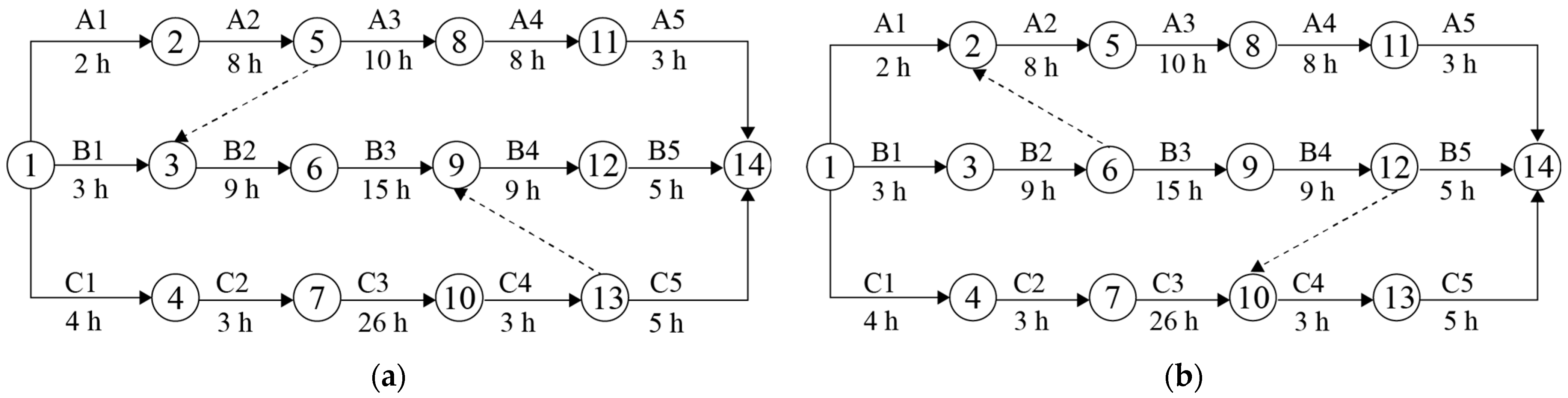
Below, a simple example is provided to illustrate the advantage of WTC in waiting time calculation and the necessity of considering transshipment sequence selection. Cargoes from A, B, and C are transported to a destination via upstream stations (1 and 2) and downstream stations (3 and 4). A hub allocation result is shown in Table 3 where A and B share 2, while B and C share 4. Therefore, congestion may occur at 2 and 4, necessitating the determination of the transshipment sequence. According to WTC, the transshipment sequence at 4 is determined by the FCFS rule, so it is only necessary to select transshipment sequences for A and B at 2. From Table 3, it can be seen that there are two feasible sequencing schemes for A→B and B→A. The bipartite network diagrams for these two schemes are shown in Figure 2a and Figure 2b, respectively. Taking A in the two figures as an example, the solid arrows and the labels above them (A1, A2, A3, A4, and A5) represent the operations ①, ②-2, ③, ④-2, and ⑤ for A, respectively; the numbers below represent the time required to complete the operations, respectively. The symbols for B and C have similar meanings. The dashed arrows in the two figures represent transshipment sequences at hubs.
Table 3.
Hub allocation result.
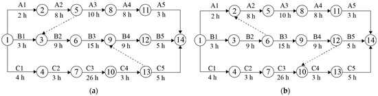
Figure 2.
The bipartite network diagrams of the two transshipment sequencing schemes: (a) A→B; (b) B→A.
From Figure 2a, A2 is the immediate predecessor activity of B2. Since A arrives at 2 before B, and C arrives at 4 before B, Figure 2a can be considered adopting the FCFS rule to determine the transshipment sequence. Unlike Figure 2a, in Figure 2b, B2 is adjusted to be the immediate predecessor activity of A2, resulting in B arriving at 4 before C; consequently, B4 is adjusted to be the immediate predecessor activity of C4. Set = 0, and use WTC to calculate , , and for Figure 2a,b, with the results shown in columns 3, 4, and 5 of Table 4. Then, replace and with the average waiting time and , respectively, then calculate the average end moment () with the results shown in columns 6, 7, and 8 of Table 4.
Table 4.
The results of the two schemes.
From Table 4, it can be seen that when using , the makespans of Figure 2a and Figure 2b are 50 h and 44 h, respectively, so Figure 2b is superior to Figure 2a. However, when using , the makespans of Figure 2a and Figure 2b are 45.5 h and 47.5 h, respectively, so Figure 2a is superior to Figure 2b. That is, different waiting time estimate methods can lead to an opposite decision here. If the average waiting time is used for makespan calculation, the FCFS rule is the best sequencing rule, no specialized decision is needed for the transshipment sequence selection. However, if WTC is used for makespan calculation, the makespan of Figure 2b reduces by 6 h compared to Figure 2a, necessitating a special transshipment sequence selection decision. This suggests that introducing WTC for minimum waiting time calculation and transshipment sequence selection can result in a higher-quality multimodal transport scheme, thereby confirming the effectiveness of the simulation approach.
3.2. Memetic Algorithm for Solving ITRTSP
From Section 2.1, WTC can solve for based on any given transshipment sequence at an upstream station. Therefore, as long as all possible transshipment sequences are traversed, a better sequencing scheme can be obtained theoretically (at least not inferior to the FCFS rule). However, since the two-stage HFSP is an NP-hard problem [45], its global optimum solution is usually difficult to obtain within a limited decision time when the solution space size is large. In such a case, heuristics is usually a more reasonable option. In fact, the FCFS rule is one of the important heuristics for solving the sequencing problem. However, further searching for feasible transshipment sequences based on hub allocation will make the solution space size grow exponentially. If the heuristics are not properly designed, the result may be inferior to the FCFS rule and adversely affect the road–rail multimodal transport scheme. Thus, special research on heuristics is needed to solve ITRTSP.
As mentioned above, ITRTSP can be transformed into a two-stage HFSP with transport constraints. Generally speaking, a solution to an HFSP mainly consists of machine allocation and processing sequence [9]. Existing heuristic methods [40,46,47,48] usually first encode the solution as processing sequences of jobs and then use machine allocation rules to decode the given processing sequence and calculate the makespan. For example, in the memetic algorithm framework (referred to as Framework 1) designed by Lei et al. [40], algorithms such as NEH, IG, and GA are for the outer layer to generate and optimize processing sequences; while algorithms such as IMPT, ECTT, and GAMT are for the inner layer to find better machine allocation schemes for the processing sequences generated by the outer layer. The memetic algorithm integrates the strengths of global and local search, allowing for the exploration of multiple high-quality regions within the solution space [40,49]. This approach leads to more precise identification of optimal solutions. Due to its effectiveness in handling complex problems, this paper also designs nested solution methods based on the memetic algorithm framework. The difference is that the methods in this paper first encode multimodal transport schemes as hub allocations, and then decode them by selecting an appropriate transshipment sequence for each; that is, the memetic algorithm framework in this paper is constructed with hub allocation as the outer layer and transshipment sequence selection as the inner layer (referred to as Framework 2, see Figure 3). As the genetic algorithm (GA) is widely used due to its superior global search performance in minimizing makespan in HFSP [50,51], the nested genetic algorithm (abbreviated as GA_GA) is used to illustrate the solution process of Framework 2. The detailed calculation process of GA_GA is as follows.
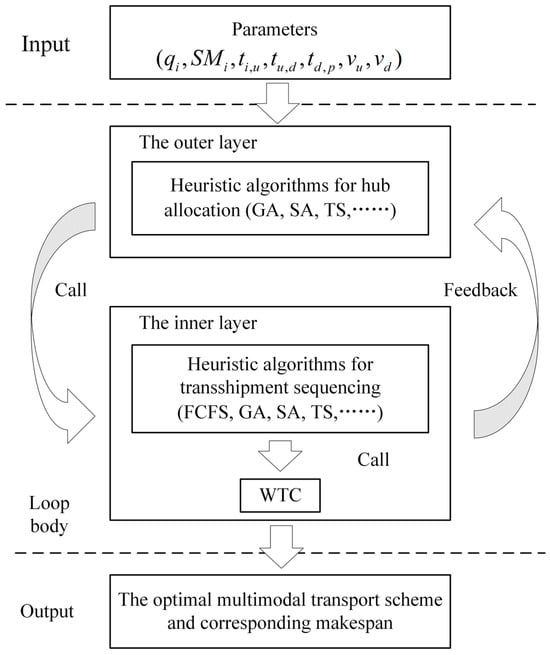
Figure 3.
The memetic algorithm framework.
Step 1: Set parameters. Firstly, input the data, including quantities and transport start moments of all cargoes, the road and rail transport times, and the transshipment efficiencies at upstream and downstream stations. Then, set the inner and outer layer algorithms parameters, including maximum genetic generations, population sizes, crossover and mutation probabilities, etc.
Step 2: Construct an initial outer layer population. Generate an initial population of N chromosomes as the current outer layer population. Each chromosome consists of 2|R| genes; the first |R| genes are sequenced by the origin numbers, with the i-th gene indicating u chosen for i. The second |R| genes are also sequenced by the origin numbers, with the |R|+i-th gene indicating d chosen for i. To comply with Equations (2) and (3), the first |R| genes are randomly selected from U, and the second |R| genes are randomly selected from D. For example, a chromosome in the outer layer population of the example given in Table 3 is shown in Figure 4a, which indicates that A, B, and C are transported to the destination via upstream stations 2, 2, 1 and downstream stations 3, 4, 4, respectively.
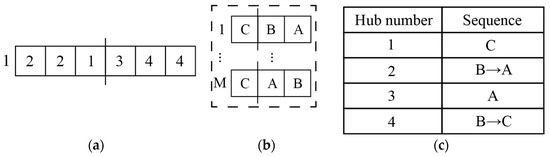
Figure 4.
Chromosome encoding: (a) The outer layer chromosome; (b) The inner layer population; (c) The transshipment sequence scheme of the first inner layer chromosome.
Step 3: Perform crossover and mutation for the chromosomes in the current outer layer population. Then N new chromosomes are generated. To ensure the feasibility of the new chromosomes, segmented multipoint crossover and mutation are separately applied to the first |R| and the second |R| genes. For example, in the example given in Table 3, perform multipoint crossover by swapping corresponding genes (Figure 5a). After crossover, apply segmented mutation to the new chromosomes (Figure 6a). Merge these chromosomes after crossover and mutation with the original chromosomes from the current population to form a new outer layer population.
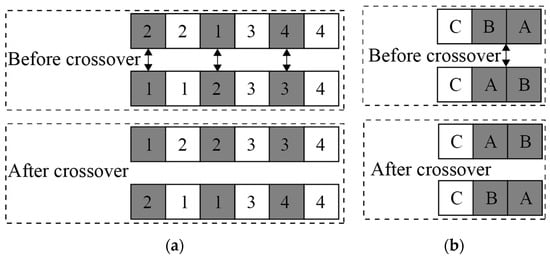
Figure 5.
Crossover: (a) Crossover for the outer layer chromosomes; (b) Crossover for the inner layer chromosomes.
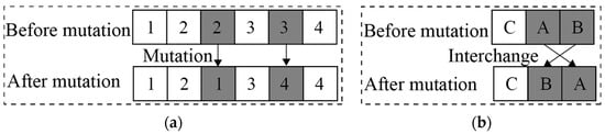
Figure 6.
Mutation: (a) Mutation for the outer layer chromosome; (b) Mutation for the inner layer chromosome.
Step 4: Inner layer algorithms.
Step 4.1: Construct initial inner layer populations. Transfer the information of the current outer layer population to the inner layer, creating an initial inner layer population for each outer layer chromosome (total 2N inner layer populations), and select one population n () as the current inner layer population. Each inner layer population consists of M chromosomes, each chromosome containing |R| genes. The gene sequence represents the transshipment sequence at an upstream station, with each gene indicating that i needs to be loaded (onto trains) in that sequence. To comply with Equations (5) and (6), the genes of each inner layer chromosome should be restricted. First, similar to WTC, divide R into |U| disjoint subsets (, the union of all is R) based on the first |R| genes (selection results of upstream stations) of outer layer chromosome n. is the set of all that select u. Second, group the gene positions for each inner layer chromosome, assigning || gene positions to each (if = Φ, then || = 0, meaning no gene positions are assigned to u). Finally, for each inner layer chromosome, randomly draw elements from without replacement to fill the gene positions, generating the transshipment sequences at each upstream station that satisfies Equations (4)–(10). For example, in the outer layer chromosome shown in Figure 4a, = {C} and = {A, B} are the groups for the upstream stations. Assign gene position 1 of the inner chromosome to and gene positions 2 and 3 to . By performing random draws, the initial inner layer population can be generated as shown in Figure 4b (for instance, Figure 4c shows the draw result of the first chromosome in Figure 4b).
Step 4.2: Based on the current inner population n, perform crossover and mutation to generate M new chromosomes. To ensure the feasibility of these new chromosomes, only perform crossover and mutation within the same subset . Taking the two chromosomes numbered 1 and M in Figure 4b as an example, when performing crossover on , only the gene positions 2 and 3 of the two chromosomes can be crossed, resulting in two new chromosomes, as shown in Figure 5b. After crossover, perform mutation on by swapping gene positions 2 and 3 to form a new chromosome, as shown in Figure 6b. Merge the new M chromosomes with the original chromosomes to form a new current inner layer population with the 2M chromosomes.
Step 4.3: Calculate fitness values of inner layer chromosomes. First, construct a multimodal transport scheme consisting of outer layer chromosome n and inner layer chromosome m . Second, apply WTC to calculate in . Finally, formulate the inner layer fitness function:
where is the fitness value of . Substituting and into Equation (24) can obtain the . Repeat this step for all 2M chromosomes of the current inner layer population.
Step 4.4: Determine whether the current inner population n has reached its maximum generation. If not, proceed to Step 4.5; otherwise, let be equal to the , which has the maximum value of in the current inner layer population, and record its makespan. Set it as the final transport scheme for the outer layer chromosome n, and proceed to Step 4.6.
Step 4.5: Select the inner layer offspring. Applying elite tournament mode, M chromosomes are selected from the current inner layer population to form a new inner layer offspring population, which is returned as the current inner layer population to Step 4.2.
Step 4.6: Iterate over all inner layer populations. Repeat Steps 4.2 to 4.5 for all inner layer populations to obtain a set of optimized transport schemes and corresponding makespan for the outer layer population. Then proceed to Step 5.
Step 5: Outer layer chromosome fitness values calculation. Construct the outer layer fitness function:
where represents the fitness value of outer layer chromosome n, and represents the makespan of the transport scheme . Applying Equation (25), fitness values of all current outer layer chromosomes can be obtained.
Step 6: Determine whether the current outer layer population has reached its maximum generation. If not, proceed to Step 7; otherwise, select and record with the minimum makespan from . Set it as the optimal scheme and proceed to Step 8.
Step 7: Select the outer layer offspring. Applying elite tournament mode, N chromosomes are selected from the current outer layer population to form a new outer layer offspring population, which is returned as the current outer layer population to Step 3.
Step 8: End the calculation and output .
4. Example Experiments
4.1. Background of Examples
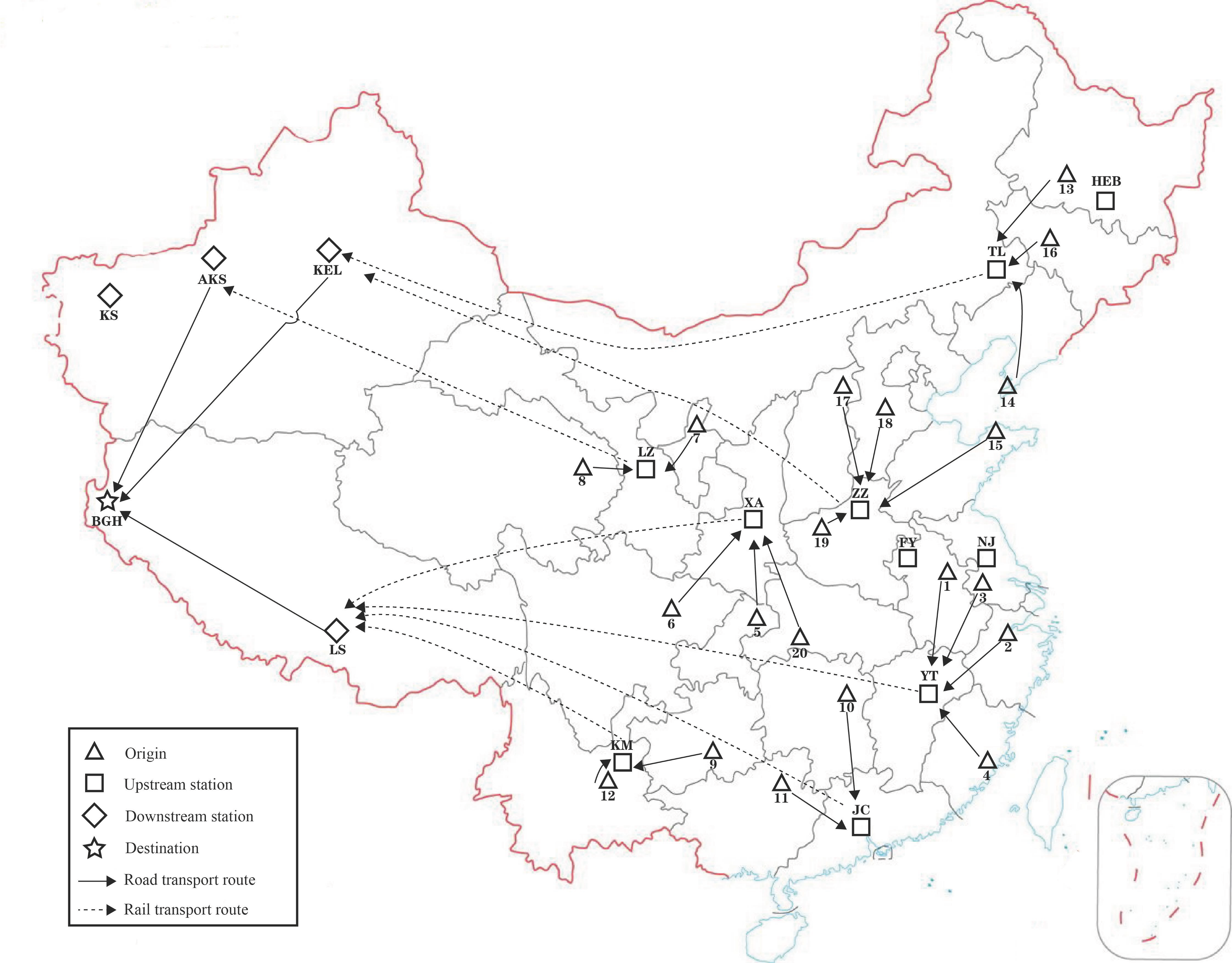
Below, this paper presents some examples based on China’s inland road–rail multimodal transport network to examine the role of transshipment sequence selection in congestion control. To address potential regional armed conflicts, the road–rail multimodal transport network will transport military equipment to the border of China. The origins, upstream stations, downstream stations, and a destination are shown in Figure 7. The transport distances are provided in Table 5, Table 6 and Table 7. The transport speeds in operations ①, ③, and ⑤ are set to 40 km/h, 60 km/h, and 25 km/h, respectively. The numerical experiments will be conducted based on this network. All experiments were performed on a DELL computer with an Intel(R) Core (TM) i7-7500U CPU @ 2.70 GHz 2.90 GHz, 8.00 GB of RAM, running Windows 10 and Python 3.7. The computation time limit for all algorithms is set to 3600 s.

Figure 7.
The road–rail multimodal transport network. Numbers 1–20 denote origins, and letter abbreviations represent upstream and downstream stations.
Table 5.
The distances (km) between origins and upstream stations.
Table 6.
The distances (km) between upstream and downstream stations.
Table 7.
The distances (km) between upstream stations and the destination.
4.2. Algorithm Performance Testing
Based on the multimodal transport network presented in Section 3.1, twenty-two examples were designed. The quantities of equipment at the twenty origins (see Table 8, ranging between 400 and 900 units) and the transshipment efficiencies of eight upstream stations (see Table 9, ranging between 2 and 30 units/h) and three downstream stations (see Table 10, ranging between 2 and 30 units/h) were randomly generated. Then, twelve small-scale examples (tests 1 to 12, see columns 1 to 4 in Table 11) and ten larger-scale examples (tests 13 to 22, see columns 1 to 4 in Table 12) were designed. Test 1 selected origins 1 to 5, upstream stations TL and LZ, as well as downstream stations AKS and KEL. As the scale of the examples gradually increased, the origins were added sequentially according to the rows in Table 5, and upstream and downstream stations were added sequentially according to the columns in Table 6 and Table 7, respectively. For example, test 2 added upstream station NJ to test 1, test 3 added origin 6 to test 1, and so on. The GA_GA was used to solve these examples with each calculated ten times. The results are shown in columns 5 and 6 of Table 11 and Table 12, where Obj and Cpu represent the average objective value and average computation time of a single experiment, respectively (in all subsequent experiments, Obj and Cpu are the averages of ten repeated calculations). The parameters of GA_GA were set as follows. The outer layer has a population size of 10, a crossover probability of 0.9, a mutation probability of 0.1, and a maximum number of generations of 100. The inner layer has a population size of 20, a crossover probability of 0.9, a mutation probability of 0.1, and a maximum number of generations of 50. Additionally, other solution methods were also designed.
Table 8.
The equipment quantities (unit).
Table 9.
The transshipment efficiencies of upstream stations (unit/h).
Table 10.
The transshipment efficiencies of downstream stations (unit/h).
Table 11.
The calculation results of small-scale examples.
Table 12.
The calculation results of large-scale examples.
- (1)
- CPLEX. Using the CPLEX solver to solve the above tests. The results are shown in columns 7, 8, and 9 of Table 11 and Table 12, where Gap represents the percentage difference of Objs between GA_GA and the algorithm compared with GA_GA. , where is the Obj of GA_GA (e.g., column 7 in Table 11), and is the Obj of the algorithm being compared with GA_GA. For example, in Table 11 for test 12, the Gap between CPLEX and GA_GA is calculated as (732.46–739.29)/732.46 × 100 = −0.93%. Hereafter, each Gap is calculated in this manner.
- (2)
- IG+ECTT. Based on Framework 1, proposed in Ref. [40], the above examples were solved with transshipment sequence selection as the outer layer and hub allocation as the inner layer. It should be noted that although Ref. [40] designed seven different solution methods, its experimental results showed that the combination of the iterated greedy algorithm and the earliest completion time with transport (IG+ECTT) is the most effective. Therefore, we compare IG+ECTT with GA_GA in our experiments. The results are shown in columns 10 to 12 of Table 11 and Table 12.
- (3)
- Other algorithms. Due to the extensive application of simulated annealing (SA) and tabu search (TS) in solving HFSP [36,52], they are selected to design single-layer solution methods along with GA, where both hub allocation and transshipment sequence selection are generated simultaneously during encoding. Furthermore, based on Framework 2 (see Figure 3), four algorithms (SA_GA, TS_GA, GA_SA, and GA_TS) were also proposed. SA_GA means that the outer layer algorithm is SA while the inner layer algorithm is GA, and so on for the other three algorithms. The data from tests 13 to 22 were input into the seven algorithms and compared with GA_GA, with the results shown in Table 13.
Table 13. The Gaps (%) between other algorithms and GA_GA.
4.3. Comparison with the FCFS Rule
As mentioned, existing studies mainly adopt the FCFS rule for transshipment sequencing. To demonstrate the differences between the method proposed in this paper and the FCFS rule, the examples in Section 3.1 were refined according to the actual conditions of transshipment hubs. The transshipment efficiencies of the upstream and downstream stations (see Table 14 and Table 15) were determined based on the “Railway Station Classification Rating Method” issued by the Ministry of Transport of the People’s Republic of China. The quantity of equipment at each origin was regenerated (see Table 16, with a total of 7000 units). Keeping the outer layer algorithm described in Section 3.2 unchanged, the inner layer algorithm (Step 4) was modified to use the FCFS rule for solving (abbreviated as GA_FCFS). The data in Table 14 and Table 16 were input into GA_GA and GA_FCFS for calculation, and the resulting multimodal transport schemes are shown in columns 2 to 5 of Table 17. To show the differences, columns 6 and 7 of Table 17 present a multimodal transport scheme [M], where hub allocation is the same as GA_GA, but transshipment sequence is determined by the FCFS rule.
Table 14.
The refined transshipment efficiencies of upstream stations (unit/h).
Table 15.
The refined transshipment efficiencies of downstream stations (unit/h).
Table 16.
The regenerated equipment quantities (unit).
Table 17.
The road–rail multimodal transport schemes.
Furthermore, the sensitivity analysis of equipment quantity and transshipment efficiency at hubs was conducted. Initially, four examples were considered with varying equipment quantities (7000, 9000, 11,000, and 13,000 units). GA_GA, IG+ECTT, and GA_FCFS were used to calculate these examples, with the results shown in Figure 8. Taking the scale of 11,000 units as an example, the average time consumed in each operation by GA_GA and GA_FCFS is presented in Figure 9. In Figure 9, denotes the average time by all equipment in operation k (k {1, 2, …, 7}). Subsequently, with a fixed equipment quantity of 11,000 units, six examples (see columns 2 and 3 of Table 18) were designed based on Table 14 and Table 15 by enhancing transshipment efficiencies at upstream stations ([C1]) and downstream stations ([C2]). Upstream stations FY, KM, and TL were selected, along with downstream stations KS, AKS, and LS, with enhancing transshipment efficiencies through equal distribution. For example, in the first example of [C1] (row 3 of Table 18), the total increase for the three upstream stations is 15 units/h, i.e., FY, KM, and TL increase 5 units/h, respectively (compared to the data in Table 14). GA_GA, IG+ECTT, and GA_FCFS were employed to calculate these examples, with the results detailed in columns 4 to 8 of Table 18.
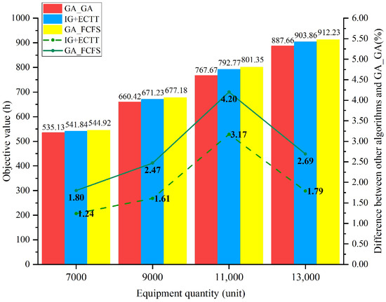
Figure 8.
The sensitivity analysis results of equipment quantity.
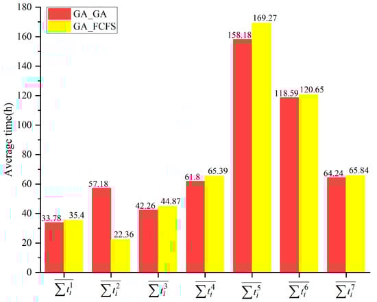
Figure 9.
The average time consumed in each operation.
Table 18.
The sensitivity analysis results of transshipment efficiency.
5. Results Analysis
5.1. Comparative Analysis of Algorithm Performance
- (1)
- CPLEX. Table 11 shows that the Objs of CPLEX are the same as GA_GA in tests 1 to 6, while they are slightly lower than GA_GA in tests 7 to 12 (see test 12 in Table 11, the maximum Gap is –0.93%). Comparing columns 6 and 8 of Table 11, it is evident that, the Cpus of CPLEX are lower than GA_GA in tests 1 to 7 (with a maximum difference of about 60 s in test 6), while they exceed GA_GA in tests 8 to 12. Moreover, it fails to find the optimal solutions within the time limit in tests 10 to 12. In contrast, the maximum Cpu of GA_GA is only about 227 s in test 12, showing a significantly less increase compared to CPLEX. As the solution space expands further (as seen in Table 12, tests 13 to 22), GA_GA consistently achieves lower Objs than CPLEX within the time limit (see column 9 of Table 12). Furthermore, the Gaps between CPLEX and GA_GA show an increasing trend (see Table 12), and the maximum is about 15% (see test 22). Column 8 of Table 12 also indicates that the Cpus of CPLEX reach the time limit, whereas the maximum of GA_GA is only 962.61 s (see test 22).
- (2)
- IG+ECTT. Comparing columns 5 and 10 of Table 11, it is found that the Objs of IG+ECTT are the same as GA_GA in tests 1 to 4, while they are slightly higher than GA_GA in tests 5 to 12, with the maximum Gap being 0.88% (see test 12). Comparing columns 6, 8, and 11 of Table 11, it can be observed that the Cpus of IG+ECTT are slightly higher than CPLEX (but lower than GA_GA) only in test 1 and test 2, while in tests 3 to 12, they are significantly lower than GA_GA and CPLEX. In tests 13 to 22, the Gaps of IG+ECTT also increase (see column 12 of Table 12), but the values are significantly less than CPLEX (with a maximum of about 4.04% in test 22). However, the Cpus of IG+ECTT in Table 12 are significantly lower than GA_GA (with a maximum of only 33.76 s in test 22).
- (3)
- Other algorithms. The Gaps of IG+ECTT are lower than GA, SA, and TS (see columns 2, 3, and 4 of Table 13). The Cpus of the three algorithms are roughly the same as IG+ECTT (with a maximum of about 34 s in test 22), significantly faster than GA_GA (962 s). The Objs of SA_GA, TS_GA, GA_SA, and GA_TS (see columns 5, 6, 7, and 8 of Table 13) are lower than IG+ECTT. The Cpus of these four algorithms are comparable to GA_GA (for example, in test 22, their Cpus are about 916 s, 978 s, 923 s, and 969 s, respectively), and are all significantly higher than IG+ECTT.
It can be seen that GA_GA has the best performance in reducing Obj. SA_GA, TS_GA, GA_SA, and GA_TS show clear advantages over single-layer algorithms in reducing Obj, although it does not perform as well as single-layer algorithms in terms of Cpu. However, IG+ECTT shows its advantages in reducing both Obj and Cpu. These results justify the advantages of the memetic algorithm in solving ITRTSP. Among all the algorithms mentioned above, GA_GA and IG+ECTT are more effective in solving ITRTSP. If decision-makers wish to minimize the makespan, GA_GA is preferable. If they want to minimize decision-making time, IG+ECTT may be a better choice. Additionally, although IG+ECTT saves decision-making time, the amount saved is significantly less than the makespan saved by GA_GA, SA_GA, TS_GA, GA_SA, and GA_TS. This indicates that, in the examples of this paper, Framework 2 is more effective than Framework 1. Although a little computation time is sacrificed, Framework 2 can significantly shorten makespan and improve emergency transport efficiency.
5.2. Comparative Analysis with the FCFS Rule
In Table 17, GA_GA saves 9.42 h compared to GA_FCFS, and GA_FCFS saves 14.60 h compared to [M]. In fact, the results of the ten examples in Figure 8 and Table 18 also exhibit similar characteristics to Table 17 (Due to limitations on space, this paper only takes Table 17 as an example). In other words, in these ten examples, the Objs of GA_GA and IG+ECTT are lower than GA_FCFS; however, if the hub allocation results of GA_GA are used with the FCFS rule, the Objs are higher than GA_FCFS. Further analysis for intermediate data (e.g., Figure 9) reveals that the average time consumed in operation ②-1 by GA_GA is significantly longer than by GA_FCFS while the average times consumed in operations ①, ②-2, ③, ④-1, ④-2, and ⑤ are all shorter than by GA_FCFS. These results indicate that transshipment sequence selection at upstream stations is the key reason that GA_GA and IG+ECTT outperform GA_FCFS. Although it increases the waiting time for partial equipment at upstream stations, it reduces the transport time, the loading and unloading time, and the waiting time at downstream stations, thereby enhancing overall multimodal transport efficiency.
In Figure 8, the Objs of GA_GA, IG+ECTT, and GA_FCFS show an upward trend with equipment quantity increasing, while the Gaps of IG+ECTT and GA_FCFS first increase and then decrease. The maximum Gaps of IG+ECTT and GA_FCF both occurring at 11,000 units, are 3.17% and 4.20%, respectively. Compared to GA_FCFS, GA_GA, and IG+ECTT save 33.68 h and 8.58 h, respectively. This indicates that for a given multimodal transport network, transport demand that is too high or too low can affect the optimization effects of transshipment sequence selection. In practice, adjusting transshipment sequences may increase the management pressure of upstream stations, such as requiring larger transshipment buffers or increasing storage and handling management costs. Therefore, comprehensively considering various transshipment sequencing rules in practice is essential. For instance, a better transshipment sequence should be considered if decision-makers wish to minimize the makespan. Conversely, if they want to reduce the management difficulty of transshipment operation while meeting time constraints, the FCFS rule might be a more favorable choice.
By examining [C1] and [C2] (Table 18), it is found that the Objs of GA_GA, IG+ECTT, and GA_FCFS, as well as the Gaps of IG+ECTT and GA_FCFS, all show decreasing trends with the improvement of transshipment efficiency. Among them, the Gaps of IG+ECTT and GA_FCFS reach their minimums in the third example of [C2] (see row 8 of Table 18), which are 0.54% and 0.93%, respectively. Compared to GA_FCFS, The Objs of GA_GA and IG+ECTT save 4.16 h and 1.75 h, respectively. This indicates that the lower the transshipment efficiency of the multimodal transport network is, the more effective the transshipment sequence selection may be.
It can also be found that when the increases in transshipment efficiency are the same, the Gaps of GA_FCFS in [C1] are larger than [C2]. For example, in rows 3 and 6 of Table 18, although the total transshipment efficiency of the multimodal transport network is 307 units/h in both examples, the Gaps of GA_FCFS are 3.03% and 1.61%, respectively. In row 3, the Objs of GA_GA and IG+ECTT save 23.76 h and 6.25 h compared to GA_FCFS, respectively; whereas in row 6, savings are 9.76 h and 3.60 h, respectively. This indicates that the more significant differences in transshipment efficiency between upstream and downstream stations, the more impactful the transshipment sequence selection.
Additionally, in the ten examples of sensitivity analysis, the average Cpu of GA_FCFS is approximately 25 s, outperforming GA_GA (1138 s) and IG+ECTT (36 s). However, comparing the Objs of the three algorithms, the largest difference occurs in the third example (in Figure 8, 11,000 units) where GA_GA saves 33.68 h compared to GA_FCFS; the smallest difference occurs in the tenth example (in row 8 of Table 18) where IG+ECTT saves 1.75 h compared to GA_FCFS. These results indicate that although introducing transshipment sequence selection adds some computation time, it significantly improves multimodal transport efficiency compared to the FCFS rule.
6. Conclusions
To explore the role of transshipment scheduling at hubs in managing congestion in road–rail multimodal transport, this paper proposes a nonlinear 0–1 programming model. Through a joint decision on transport route and transshipment sequence, the waiting time can be adjusted in the model, thereby optimizing the emergency multimodal transport makespan. A key distinction from the existing literature on multimodal transport lies in that it sets specific variables and constraints to describe the impact of the transshipment sequence on waiting time. A recursive method for calculating waiting times is proposed. A memetic algorithm framework is designed with route selection as the outer layer and transshipment sequence selection as the inner layer for solving the model. Finally, using China’s inland road–rail multimodal transport network as an application context, the performance of the solution methods is validated.
From the numerical experiments, the following conclusions can be drawn. First, transshipment scheduling at hubs in managing congestion should be fully recognized in emergency road–rail multimodal transport activities. For example, congestion can be controlled by transshipment sequence selection, thereby shortening the makespan. Second, production scheduling models and methods may be reasonable and effective choices to accurately quantify the dependency between transshipment scheduling and waiting time in multimodal transport problems. Third, when solving two-stage HFSPs for real-scale examples (such as ITRTSP proposed in this paper), setting machine allocation (hub allocation) as the outer layer and job sequencing (transshipment sequencing) as the inner layer may yield better results.
The contributions of this paper to multimodal transport research are mainly summarized in three aspects. First, it proposes and demonstrates that congestion can be controlled by adjusting transshipment sequences at hubs to enhance emergency transport efficiency in multimodal transport systems. Second, it constructs a two-stage HFSP model with transport constraints to quantitatively describe the dependency between transshipment sequence selection and waiting time in road–rail multimodal transport. Third, it proposes a recursive method (WTC) for calculating minimum waiting times and designs a memetic algorithm framework for solving ITRTSP.
This study aims to explore the impact of transshipment sequencing as one aspect of the operation scheduling at hubs on emergency transport efficiency in multimodal transport network settings. However, the study has certain limitations. First, it focuses solely on the dependency between transshipment sequencing and waiting time. Second, it only uses common search algorithms in HFSP, due to its early stage in applying HFSP modeling concepts to manage congestion in road–rail multimodal transport systems. Future research should build on this work by fully considering other aspects of operation scheduling at hubs, such as more complex transshipment planning operations [23,24], yard storage strategies [25], and traffic management [27]. Meanwhile, exploring more advanced optimization algorithms or the application of simulation models is also set to be a major area of interest.
Author Contributions
Conceptualization, S.T.; methodology, S.T.; software, S.T., S.L. and C.L.; validation, S.T. and S.L.; investigation, S.L. and Z.L.; data curation, S.L. and C.L.; writing—original draft preparation, S.T.; writing—review and editing, S.T. and S.L.; visualization, S.L. and Z.L.; supervision, Z.L. All authors have read and agreed to the published version of the manuscript.
Funding
This research received no external funding.
Institutional Review Board Statement
Not applicable.
Informed Consent Statement
Not applicable.
Data Availability Statement
The original contributions presented in the study are included in the article, further inquiries can be directed to the corresponding author.
Conflicts of Interest
The authors declare no conflicts of interest.
References
- Zheng, Y.-J. Emergency Train Scheduling on Chinese High-Speed Railways. Transp. Sci. 2018, 52, 1077–1091. [Google Scholar] [CrossRef]
- Zheng, Y.-J.; Ling, H.-F. Emergency Transportation Planning in Disaster Relief Supply Chain Management: A Cooperative Fuzzy Optimization Approach. Soft Comput. 2013, 17, 1301–1314. [Google Scholar] [CrossRef]
- Zheng, Y.-J.; Ling, H.-F.; Shi, H.-H.; Chen, H.-S.; Chen, S.-Y. Emergency Railway Wagon Scheduling by Hybrid Biogeography-Based Optimization. Comput. Oper. Res. 2014, 43, 1–8. [Google Scholar] [CrossRef]
- Zheng, Y.-J.; Zhang, M.-X.; Ling, H.-F.; Chen, S.-Y. Emergency Railway Transportation Planning Using a Hyper-Heuristic Approach. IEEE Trans. Intell. Transp. Syst. 2015, 16, 321–329. [Google Scholar] [CrossRef]
- Archetti, C.; Peirano, L.; Speranza, M.G. Optimization in Multimodal Freight Transportation Problems: A Survey. Eur. J. Oper. Res. 2022, 299, 1–20. [Google Scholar] [CrossRef]
- Haghani, A.; Oh, S.C. Formulation and Solution of a Multi-Commodity, Multi-Modal Network Flow Model for Disaster Relief Operations. Transp. Res. Part A Policy Pract. 1996, 30, 231–250. [Google Scholar] [CrossRef]
- Ma, K.; Yan, H.; Ye, Y.; Zhou, D.; Ma, D. Critical Decision-Making Issues in Disaster Relief Supply Management: A Review. Comput. Intell. Neurosci. 2022, 2022, 1105839. [Google Scholar] [CrossRef]
- Ishfaq, R.; Sox, C.R. Design of Intermodal Logistics Networks with Hub Delays. Eur. J. Oper. Res. 2012, 220, 629–641. [Google Scholar] [CrossRef]
- Ozdamar, L.; Demir, O. A Hierarchical Clustering and Routing Procedure for Large Scale Disaster Relief Logistics Planning. Transp. Res. Part E Logist. Transp. Rev. 2012, 48, 591–602. [Google Scholar] [CrossRef]
- Bayram, V.; Yildiz, B.; Farham, M.S. Hub Network Design Problem with Capacity, Congestion, and Stochastic Demand Considerations. Transp. Sci. 2023, 57, 1276–1295. [Google Scholar] [CrossRef]
- Campbell, J.F. Location and Allocation for Distribution Systems with Transshipments and Transportion Economies of Scale. Ann. Oper. Res. 1992, 40, 77–99. [Google Scholar] [CrossRef]
- Ebery, J.; Krishnamoorthy, M.; Ernst, A.; Boland, N. The Capacitated Multiple Allocation Hub Location Problem: Formulations and Algorithms. Eur. J. Oper. Res. 2000, 120, 614–631. [Google Scholar] [CrossRef]
- Taherkhani, G.; Alumur, S.A.; Hosseini, M. Benders Decomposition for the Profit Maximizing Capacitated Hub Location Problem with Multiple Demand Classes. Transp. Sci. 2020, 54, 1446–1470. [Google Scholar] [CrossRef]
- Contreras, I.; Cordeau, J.-F.; Laporte, G. Exact Solution of Large-Scale Hub Location Problems with Multiple Capacity Levels. Transp. Sci. 2012, 46, 439–459. [Google Scholar] [CrossRef]
- Tanash, M.; Contreras, I.; Vidyarthi, N. An Exact Algorithm for the Modular Hub Location Problem with Single Assignments. Comput. Oper. Res. 2017, 85, 32–44. [Google Scholar] [CrossRef]
- Butun, C.; Petrovic, S.; Muyldermans, L. The Capacitated Directed Cycle Hub Location and Routing Problem under Congestion. Eur. J. Oper. Res. 2021, 292, 714–734. [Google Scholar] [CrossRef]
- Guldmann, J.M.; Shen, G. A General Mixed Integer Nonlinear Optimization Model for Hub Network Design. In Proceedings of the 44th North American meeting of the Regional Science Association International, Buffalo, NY, USA, 6–9 November 1997. [Google Scholar]
- de Camargo, R.S.; de Miranda, G.; Ferreira, R.P.M. A Hybrid Outer-Approximation/Benders Decomposition Algorithm for the Single Allocation Hub Location Problem under Congestion. Oper. Res. Lett. 2011, 39, 329–337. [Google Scholar] [CrossRef]
- Azizi, N.; Vidyarthi, N.; Chauhan, S.S. Modelling and Analysis of Hub-and-Spoke Networks under Stochastic Demand and Congestion. Ann. Oper. Res. 2018, 264, 1–40. [Google Scholar] [CrossRef]
- Zukhruf, F.; Frazila, R.B.; Burhani, J.T.; Prakoso, A.D.; Sahadewa, A.; Langit, J.S. Developing an Integrated Restoration Model of Multimodal Transportation Network. Transp. Res. Part D Transp. Environ. 2022, 110, 103413. [Google Scholar] [CrossRef]
- Ertem, M.A.; Akdogan, M.A.; Kahya, M. Intermodal Transportation in Humanitarian Logistics with an Application to a Turkish Network Using Retrospective Analysis. Int. J. Disaster Risk Reduct. 2022, 72, 102828. [Google Scholar] [CrossRef]
- Li, C.; Han, P.; Zhou, M.; Gu, M. Design of Multimodal Hub-and-Spoke Transportation Network for Emergency Relief under COVID-19 Pandemic: A Meta-Heuristic Approach. Appl. Soft Comput. 2023, 133, 109925. [Google Scholar] [CrossRef] [PubMed]
- Sun, D.; Tang, L.; Baldacci, R.; Lim, A. An Exact Algorithm for the Unidirectional Quay Crane Scheduling Problem with Vessel Stability. Eur. J. Oper. Res. 2021, 291, 271–283. [Google Scholar] [CrossRef]
- Li, X.; Otto, A.; Pesch, E. Solving the Single Crane Scheduling Problem at Rail Transshipment Yards. Discret. Appl. Math. 2019, 264, 134–147. [Google Scholar] [CrossRef]
- Zając, M. The Model of Reducing Operations Time at a Container Terminal by Assigning Places and Sequence of Operations. Appl. Sci. 2021, 11, 12012. [Google Scholar] [CrossRef]
- Rožić, T.; Ivanković, B.; Bajor, I.; Starčević, M. A Network-Based Model for Optimization of Container Location Assignment at Inland Terminals. Appl. Sci. 2022, 12, 5833. [Google Scholar] [CrossRef]
- Gao, Y.; Chen, C.-H.; Chang, D. A Machine Learning-Based Approach for Multi-AGV Dispatching at Automated Container Terminals. J. Mar. Sci. Eng. 2023, 11, 1407. [Google Scholar] [CrossRef]
- Gao, Y.; Zhen, L. A Decision Framework for Decomposed Stowage Planning for Containers. Transp. Res. Part E Logist. Transp. Rev. 2024, 183, 103420. [Google Scholar] [CrossRef]
- Kizilay, D.; Eliiyi, D.T.; Van Hentenryck, P. Constraint and Mathematical Programming Models for Integrated Port Container Terminal Operations. In Integration of Constraint Programming, Artificial Intelligence, and Operations Research; Van Hoeve, W.-J., Ed.; Springer International Publishing: Cham, Germany, 2018; Volume 10848, pp. 344–360. [Google Scholar]
- Marianov, V.; Serra, D. Location-Allocation of Multiple-Server Service Centers with Constrained Queues or Waiting Times. Ann. Oper. Res. 2002, 111, 35–50. [Google Scholar] [CrossRef]
- Elhedhli, S.; Wu, H. A Lagrangean Heuristic for Hub-and-Spoke System Design with Capacity Selection and Congestion. INFORMS J. Comput. 2010, 22, 282–296. [Google Scholar] [CrossRef]
- Assadipour, G.; Ke, G.Y.; Verma, M. Planning and Managing Intermodal Transportation of Hazardous Materials with Capacity Selection and Congestion. Transp. Res. Part E Logist. Transp. Rev. 2015, 76, 45–57. [Google Scholar] [CrossRef]
- Alumur, S.A.; Nickel, S.; Rohrbeck, B.; Saldanha-da-Gama, F. Modeling Congestion and Service Time in Hub Location Problems. Appl. Math. Model. 2018, 55, 13–32. [Google Scholar] [CrossRef]
- Ruiz, R.; Vázquez-Rodríguez, J.A. The Hybrid Flow Shop Scheduling Problem. Eur. J. Oper. Res. 2010, 205, 1–18. [Google Scholar] [CrossRef]
- Hidri, L.; Elkosantini, S.; Mabkhot, M.M. Exact and Heuristic Procedures for the Two Center Hybrid Flow Shop Scheduling Problem with Transportation Times. IEEE Access 2018, 6, 21788–21801. [Google Scholar] [CrossRef]
- Hosseini, A.; Otto, A.; Pesch, E. Scheduling in Manufacturing with Transportation: Classification and Solution Techniques. Eur. J. Oper. Res. 2024, 315, 821–843. [Google Scholar] [CrossRef]
- Li, X.; Guo, X.; Tang, H.; Wu, R.; Liu, J. An Improved Cuckoo Search Algorithm for the Hybrid Flow-Shop Scheduling Problem in Sand Casting Enterprises Considering Batch Processing. Comput. Ind. Eng. 2023, 176, 108921. [Google Scholar] [CrossRef]
- Yu, M.; Liu, X.; Xu, Z.; He, L.; Li, W.; Zhou, Y. Automated Rail-Water Intermodal Transport Container Terminal Handling Equipment Cooperative Scheduling Based on Bidirectional Hybrid Flow-Shop Scheduling Problem. Comput. Ind. Eng. 2023, 186, 109696. [Google Scholar] [CrossRef]
- Czerniachowska, K.; Lutosławski, K. Optimising Order Picking Efficiency in a Warehouse and Distribution Centre: A Flexible Flow Shop Scheduling Approach. Procedia Comput. Sci. 2023, 225, 832–841. [Google Scholar] [CrossRef]
- Lei, C.; Zhao, N.; Ye, S.; Wu, X. Memetic Algorithm for Solving Flexible Flow-Shop Scheduling Problems with Dynamic Transport Waiting Times. Comput. Ind. Eng. 2020, 139, 105984. [Google Scholar] [CrossRef]
- Lee, C.-Y.; Chen, Z.-L. Machine Scheduling with Transportation Considerations. J. Sched. 2001, 4, 3–24. [Google Scholar] [CrossRef]
- Brucker, P.; Knust, S.; Cheng, T.C.E.; Shakhlevich, N.V. Complexity Results for Flow-Shop and Open-Shop Scheduling Problems with Transportation Delays. Ann. Oper. Res. 2004, 129, 81–106. [Google Scholar] [CrossRef]
- Berghman, L.; Kergosien, Y.; Billaut, J.-C. A Review on Integrated Scheduling and Outbound Vehicle Routing Problems. Eur. J. Oper. Res. 2023, 311, 1–23. [Google Scholar] [CrossRef]
- Fu, Y.; Zhou, M.; Guo, X.; Qi, L.; Gao, K.; Albeshri, A. Multiobjective Scheduling of Energy-Efficient Stochastic Hybrid Open Shop With Brain Storm Optimization and Simulation Evaluation. IEEE Trans. Syst. Man Cybern. Syst. 2024, 54, 4260–4272. [Google Scholar] [CrossRef]
- Hoogeveen, J.A.; Lenstra, J.K.; Veltman, B. Preemptive Scheduling in a Two-Stage Multiprocessor Flow Shop Is NP-Hard. Eur. J. Oper. Res. 1996, 89, 172–175. [Google Scholar] [CrossRef]
- Behnamian, J. Decomposition Based Hybrid VNS-TS Algorithm for Distributed Parallel Factories Scheduling with Virtual Corporation. Comput. Oper. Res. 2014, 52, 181–191. [Google Scholar] [CrossRef]
- Hatami, S.; Ruiz, R.; Andres-Romano, C. Heuristics and Metaheuristics for the Distributed Assembly Permutation Flowshop Scheduling Problem with Sequence Dependent Setup Times. Int. J. Prod. Econ. 2015, 169, 76–88. [Google Scholar] [CrossRef]
- Pan, R.; Wang, Q.; Li, Z.; Cao, J.; Zhang, Y. Steelmaking-Continuous Casting Scheduling Problem with Multi-Position Refining Furnaces under Time-of-Use Tariffs. Ann. Oper. Res. 2022, 310, 119–151. [Google Scholar] [CrossRef]
- Nguyen, P.T.H.; Sudholt, D. Memetic Algorithms Outperform Evolutionary Algorithms in Multimodal Optimisation. Artif. Intell. 2020, 287, 103345. [Google Scholar] [CrossRef]
- Yu, C.; Semeraro, Q.; Matta, A. A Genetic Algorithm for the Hybrid Flow Shop Scheduling with Unrelated Machines and Machine Eligibility. Comput. Oper. Res. 2018, 100, 211–229. [Google Scholar] [CrossRef]
- Ruiz, R.; Maroto, C. A Genetic Algorithm for Hybrid Flowshops with Sequence Dependent Setup Times and Machine Eligibility. Eur. J. Oper. Res. 2006, 169, 781–800. [Google Scholar] [CrossRef]
- Lee, T.-S.; Loong, Y.-T. A Review of Scheduling Problem and Resolution Methods in Flexible Flow Shop. Int. J. Ind. Eng. Comput. 2019, 10, 67–88. [Google Scholar] [CrossRef]


Disclaimer/Publisher’s Note: The statements, opinions and data contained in all publications are solely those of the individual author(s) and contributor(s) and not of MDPI and/or the editor(s). MDPI and/or the editor(s) disclaim responsibility for any injury to people or property resulting from any ideas, methods, instructions or products referred to in the content. |
© 2024 by the authors. Licensee MDPI, Basel, Switzerland. This article is an open access article distributed under the terms and conditions of the Creative Commons Attribution (CC BY) license (https://creativecommons.org/licenses/by/4.0/).