Abstract
The joint moment is a key measurement in locomotion analysis. Transferable prediction across different subjects is advantageous for calibration-free, practical clinical applications. However, even for similar gait motions, intersubject variance presents a significant challenge in maintaining reliable prediction performance. The optimal deep learning models for ankle moment prediction during dynamic gait motions remain underexplored for both intrasubject and intersubject usage. This study evaluates the feasibility of different deep-learning models for estimating ankle moments using sEMG data to find an optimal intrasubject model against the inverse dynamic approach. We verified and compared the performance of 1302 intrasubject models per subject on 597 steps from seven subjects using various architectures and feature sets. The best-performing intrasubject models were recurrent convolutional neural networks trained using signal energy features. They were then transferred to realize intersubject ankle moment estimation.
1. Introduction
Joint moment is a key measurement in locomotion analysis, obtained through quantitative analysis. Acquiring joint kinetics is essential for understanding joints’ synergistic function, locomotion, and interaction with the surrounding environment to aid the rehabilitation process, prevent sports injuries [1], help design active exoskeletons to support the paraplegic and elderly population [2], and design active bipedal robots [3].
The main issue in this domain is that instruments that can directly measure joint moments disrupt natural movement. Inverse dynamics (ID) is the most common non-invasive method for obtaining joint moments. Its results are adopted as standard measurements in other research [4,5,6]. Nevertheless, ID requires body segment information, kinematics data, and external force data, which can be collected using gold-standard instruments consisting of motion capture systems and force plates. These systems are expensive and operate in a restricted space, which raises the need for an alternative solution.
Proper muscle and model selection are critical for accurately estimating the joint moment using surface electromyography (sEMG) signals. There are two commonly known approaches for mapping the sEMG signal to the joint moment. The first is a model-based approach achieved by constructing a neuromusculoskeletal (NMS) model that inputs sEMG signals and returns the corresponding kinematics and kinetics data. The Hill-based muscle model is the most frequently used NMS model [7,8]. However, this approach requires many anthropometric parameters for NMS model creation, and the created model will be subject-specific. The second approach is data-driven models, also known as the model-free approach, which uses machine learning (ML) or deep learning (DL) to train a model to map the sEMG signals to their corresponding joint moment. This approach requires fewer anthropometric parameters than the NMS model approach, allowing for intersubject model transfer. However, a large and clean dataset is necessary to train the model [8].
In data-driven models, extracting meaningful information related to the task is vital. Liu et al. [9] have shown that using featureless sEMG signals results in lower performance compared to using sEMG features. A key question is: which muscles and features contribute most to the training of an efficient model?
Phinyomark et al. [10] studied the properties of 37 time and frequency domain sEMG features calculated using sEMG signals for building a hand gesture classification model. They classified the time domain features into four groups based on their mathematical properties: (1) energy and complexity information methods, (2) frequency information methods, (3) prediction model methods, and (4) time-dependence methods. The features from the first group—such as mean absolute value (MAV)—and the second group—such as Zero crossing count (ZC)—performed better than those from the last group and frequency domain. Although the study by Ref. [10] was for hand classification, the feature extraction methods and categorization can be applied to lower limb sEMG signals as well.
Zhu et al. [5] trained the Elman neural network model for ankle moment estimation by extracting the root mean square (RMS) features from four muscles’ sEMG signal (biceps femoris (BF), semitendinosus (ST), vastus lateralis (VL), and gastrocnemius) as well as thigh and shank angles. Their intrasubject model achieved a normalized root mean square error (NRMSE) of .
Zhang et al. [8] trained multi-layer perception (MLP) models using three shank muscles (tibialis anterior (TA), soleus (SOL), and gastrocnemius medialis (GM)) along with the ankle angle for estimating the ankle moment. They trained different models based on different data collection methods and validated each model across seven different activities. They then compared the MLP results with an NMS model. The study found that NMS models can outperform MLP models when the sEMG signal reaches maximum levels; however, the MLP model performed better when trained on a large and varied set of trials. Their best walking model achieved a root mean square error (RMSE) of Nm/kg, but it was trained and tested on data with a fixed walking speed. When the volunteers’ walking speed was not determined, the best MLP model achieved an RMSE of Nm/kg, showing that training a model with a determined walking speed is easier than with free walking speed.
Siu et al. [11] compared the performance of MLP, neural ordinary differential equations (ODE), convolutional neural networks (CNN), and long short-term memory (LSTM) models with 30,642, 30,912, 156,264, and 32,306 parameters, respectively, for both legs’ ankle moment estimation. They used four sEMG sensors on each leg (TA, GM, ST, and vastus medialis (VM)), each equipped with accelerometers to provide additional input to the model. The LSTM model achieved the best results during walking trials, with an RMSE of Nm/kg.
In our previous study [12], we trained LSTM models to estimate knee and ankle angles and moments from both legs simultaneously, using seven sEMG signals on each leg (rectus femoris (RF), BF, VL, ST, TA, GM, and SOL) and extracted eight features per muscle. The models were trained and tested in three daily activities: (1) squat, (2) picking an object from the ground and putting it back, and (3) sitting on a chair and standing up and achieved average coefficient of determination () and , respectively, for the knee angle and moment estimation, but found some difficulties with the ankle angle and moment ( average: and , respectively). In that study, the gait was not considered.
Beyond the regression domain, Kim et al. [13] trained classification models to classify upstairs, downstairs, uphill, and downhill as well as the transition of all these tasks from and to flat ground and the flat ground classification from sEMG signals. They recorded the sEMG signals from eleven muscles (VL, VM, RF, BF, ST, TA, SOL, gastrocnemius lateral (GL) GM, flexor hallucis longus (FHL), and extensor digitorum longus (EDL)) and experimented with 33 different muscle combinations. Their best model, using all eleven muscles, achieved a classification accuracy of . Although [13] their study was for a classification task, it raised the question of whether similar results can be obtained for regression tasks. Beyond joint kinetics, sEMG signals have also been used with deep learning models, such as LSTM, to estimate ground reaction forces [14].
sEMG signals reflect muscle activation levels and, consequently, joint moments. However, activation patterns can vary between individuals and are influenced by sensor placement. Inertial measurement unit (IMU) sensors, though lacking direct muscle kinetics information, are less sensitive to these factors and benefit from the repetitive nature of gait cycles and the relationship between joint angles and moments. Mundt et al. [6] conducted a comparative intersubject study of MLP and LSTM models trained on simulated IMU. Their LSTM model outperformed the MLP model, achieving a lower NRMSE of compared to the MLP’s . Moreira et al. [15] used the subject’s anthropometrics and kinematics information from a motion capture system in a CNN model and achieved an of .
In [5,8,12], a single model architecture was employed, and features, as well as muscle selection, were determined in advance. Conversely, refs. [6,11] employed multiple model architectures but with determined features and muscle selection. Previous research has not comprehensively justified the combination of model architecture, muscles, and feature selection. Finding a transferable model presents a challenging problem and requires researching different models and techniques [16,17].
While previous studies have explored feature selection [10], muscle selection [13], or model selection [6,11], as far as we know, a comprehensive analysis encompassing all three aspects has been lacking. Additionally, our previous LSTM model [12] had difficulties estimating the ankle moment. This study aimed to bridge this gap by empirically analyzing the architecture of three distinct DL models, in conjunction with selecting muscles and extracted features. The goal is to build a transferable and generalized ankle moment estimation model during normal gait using sEMG sensors, without including kinematics or anthropometric information.
2. Materials and Methods
2.1. Data Collection
The study was conducted according to the guidelines of the Declaration of Helsinki, and approved by the ethical committee of Tohoku University under 22A-3. Seven healthy male volunteers (age: , body mass: kg, and height: cm) participated in this experiment. The experiment protocol and the study purpose were explained to all volunteers before signing a formal consent and starting the experiment.
2.1.1. Pre-Experiment
Delsys Incorporated Trigno sEMG sensors were used to record the sEMG signals from four shank muscles (tibialis anterior (TA), soleus (SOL), gastrocnemius medialis (GM), and peroneus brevis (PB) muscles) at 1111.11 Hz. Only TA contributes to ankle dorsiflexion movement, while the remaining contribute to ankle plantar flexion movement. The sensors were adhesive at the volunteer’s skin above the muscle belly following SENIAM [18] protocol for sEMG sensors arranging and placing. The placement of each sensor was then validated by asking the volunteers to perform movements to trigger maximum the sEMG activity from the targeted muscles, as recommended by SENIAM [18].
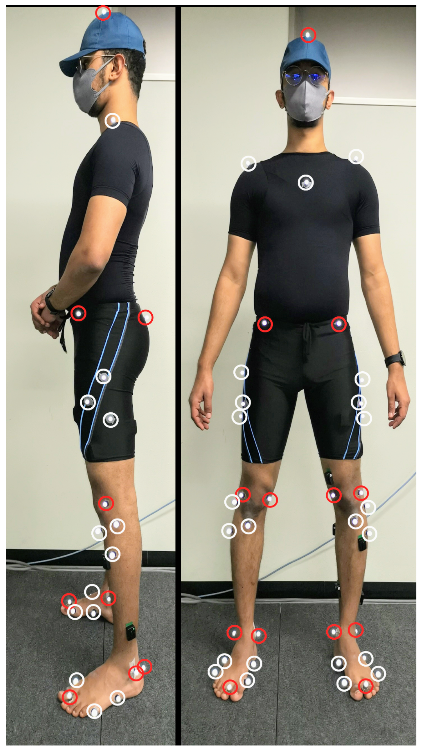
Figure 1 shows the location of thirty-nine reflective markers attached to each volunteer to track the motion using OptiTrack’s (NaturalPoint Inc. DBA, Corvallis, OR, USA) motion capture system consisting of eight reflective cameras at 100 Hz. Marker locations were chosen to align with the generic model Gait2392 provided inside OpenSim software [19,20]. The anatomical markers (red markers in Figure 1) were used to build the volunteer’s generic model and the tracking markers (the white markers in Figure 1) were used to track the motion of the volunteer. Pre-experiment the volunteers were asked to do a static reference pose (A-pose) inside the motion capture space to calibrate the location of the anatomical markers for the OpenSim model. The ground reaction force was recorded from a single Advanced Mechanical Technology Inc. force plate at 1000 Hz for all volunteers, except the first volunteer, at which the record was at 100 Hz.

Figure 1.
Anatomical (red) and tracking (white) markers.
2.1.2. Experimental Section
Data were recorded in four trials to prevent data leakage between training, validating, and testing sets. A brief break followed each trial. The first two trials lasted approximately three minutes each and were utilized for training the DL model. The remaining two trials lasted about one minute each and were employed for validating and testing the DL model.
Throughout each trial, the volunteers were asked to walk in a linear path within the motion capture space, ensuring that they consistently stepped on the force plate with their left leg before turning around and repeating the process until the end of the trial period. The length of the walking track measured approximately 3 m. In contrast, the surface area of the force plate was 0.5 m × 0.5 m. Therefore, permitting volunteers to walk at their preferred pace was deemed more efficient instead of requesting various walking speeds.
The ankle moment can be recorded during the swing phase and the stance phase on the force plate, but it can not be recorded when the volunteer foot is at the stance phase outside the force plate. Therefore, the ankle moment recording was initiated at the beginning of the swing phase, capturing the entire stance phase as the foot interacted with the force plate. Data collection continued through the succeeding swing phase, and terminating just before the start of the second stance phase. The experiment results on 430 steps for training, 84 for validation, and 83 for testing.
2.2. sEMG Data Processing
sEMG processing starts with segmenting the signals using an overlapping sliding window with a length of 200 ms and a step of 50 ms. Each segment was filtered using a 4th order Butterworth bandpass filter with a cutoff frequency of 20–450 Hz and a 50 Hz notch filter [5,8,10]. From the filtered data, we followed two approaches to extract the features, the first is by using the filtered features, and the second is by differentiating each segment to make the signal more stationary [21] using Equation (1). Features extracted from the first approach will be referred to as sEMG features, whereas the second approach features will be referred to as differentiated sEMG (DEMG) features.
is the DEMG at the time t, and is the sampling rate.
Five time-domain features were chosen based on the first three groups outlined in Phinyomark et al.’s work [10]. The selected features consisted of the root mean square (RMS) (Equation (2)), mean absolute value (MAV) (Equation (3)), and waveform length (WL) (Equation (4)) from the energy information group. Zero-crossing count (ZC) (Equation (5)) from the signal frequency information group and the fourth-order autoregressive model (AR) coefficients (Equation (6)) from the prediction model group. As a result, eight features were extracted for each sensor utilized in the study. Part of the first trial was used to normalize the features using a MinMax filter ranging from 0 to 1.
N is the number of samples, is the sample value at time t, P is the order of the AR coefficients (4 in the current study), is the pth order AR coefficients, and is the white noise.
2.3. Generic Model
The static data collected from the A-pose and volunteer’s body mass were used in OpenSim software to build the volunteer’s scaled musculoskeletal model from the generic model Gait2392 provided inside OpenSim software [19,20]. Generic model, ground reaction force (GRF) from force plate, joints angles from the inverse kinematics equation are used to solve the inverse dynamic (ID) Equation (7) and estimate ankle moment for each time frame:
N is the number of degrees of freedom, ( are the generalized position, velocity, and acceleration vectors, is the system mass matrix, is the vector of Coriolis and centrifugal forces, is the vector of gravitational forces, and is the vector of generalized forces. Ankle moments were filtered using a sixth-order Butterworth lowpass filter with a cutoff frequency of 5 Hz, downsampled to 20 Hz to match the sampling frequency of the features, and normalized by the volunteer’s body mass to reduce the variance between volunteers [22].
2.4. Dataset
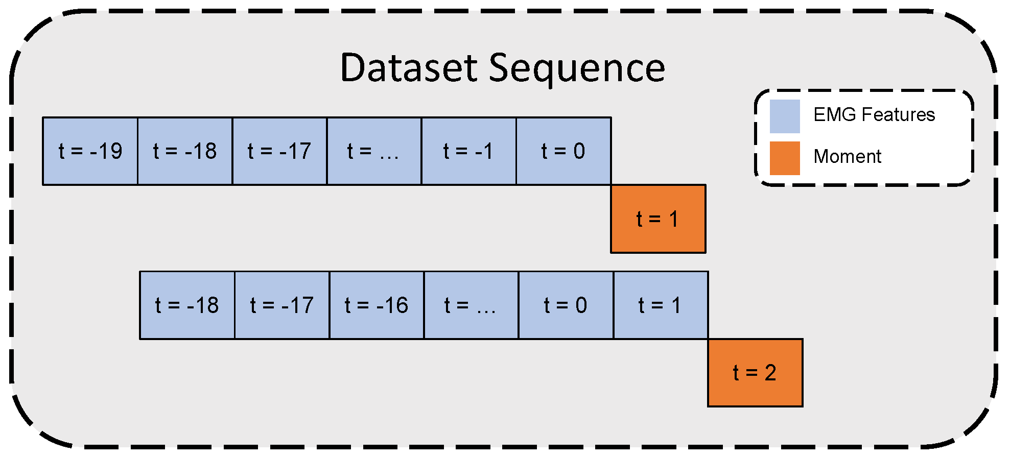
The constraint for achieving real-time prosthetic device control is for the device to respond within 300 ms [23]. In this study, for each moment value, the past 20 time-step features (equivalent to one second) were stacked together to form a time series sequence to estimate the moment at the next time step after 50 ms. Figure 2 illustrates the time-series dataset formation.
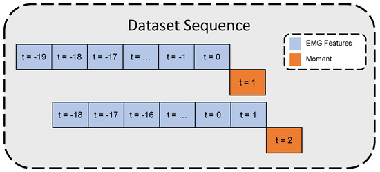
Figure 2.
Time-series dataset inputs/outputs illustration.
Since only a single force plate was used in the study, it was unattainable to continuously estimate the moment through the ID Equation (7) when the volunteer stepped outside the force plate. Accordingly, recording periods start from the swing phase before stepping on the force plate until the termination of the following swing phase. The sEMG signal maintains continuous signal tracking while the moment estimation can not be estimated while the volunteer’s leg stepped outside the force plate. Therefore, after forming the time-series dataset as in Figure 2, each sequence with a moment outside the defined recording period in Section 2.1.2 was removed from the dataset.
2.5. Deep Learning Models
DL models were built and trained using the TensorFlow-GPU framework on Python. Three different DL algorithms were targeted in this study to build the lower extremities moment estimation system. MLP, recurrent convolutional neural network (RCNN), and LSTM. All models had an input layer and a single neuron in the output layer. In between these two layers, the models were assembled as described in Table 1:

Table 1.
Models Summary and Architecture.
Nadam optimizer with modified mean squared error (MSE) loss function (Equation (8)) and mini-batch size of 8 samples was used to compile all models. The MSE in Equation (8) was doubled if the ID moment was a positive dorsiflexor moment to let the model pay attention to the small dorsiflexor moment since DL models learn from the given data to minimize the error in the training batches. The training was set to run for 1000 epochs or until convergence (based on the loss result on the validation set) with a reduced learning rate, starting from . The model with the least MSE on the validation set during the training was used on the test set to evaluate the model performance.
N is the number of samples, is the moment value at the time t, and is the predicted moment at t.
Intrasubject empirical analysis was conducted using four muscles. All trained models included the TA muscle since it is the only ankle dorsiflexion muscle selected for this study. To reduce computations, feature sets were consistently applied across muscles, and sEMG and DEMG were evaluated separately. This resulted in 434 unique feature sets. Each set was tested across three models (MLP, RCNN, and LSTM), producing 1302 models per volunteer. To prioritize computationally efficient model transfer for intersubject analysis, only the top-performing intrasubject models were selected.
2.6. Model Evaluation Metrics
The models’ performance was judged based on three evaluation metrics. (Equation (9)) to show how the estimations fit the variance in the data, RMSE (Equation (10)) to evaluate the performance of the model, and the normalized root square error (NRMSE) (Equation (11)) to compare the RMSE value across different subjects.
N is the number of samples, is the mean value of the observed y, and and are the maximum and minimum moment from the ID equation.
3. Results
3.1. Intrasubject Models
3.1.1. sEMG Models
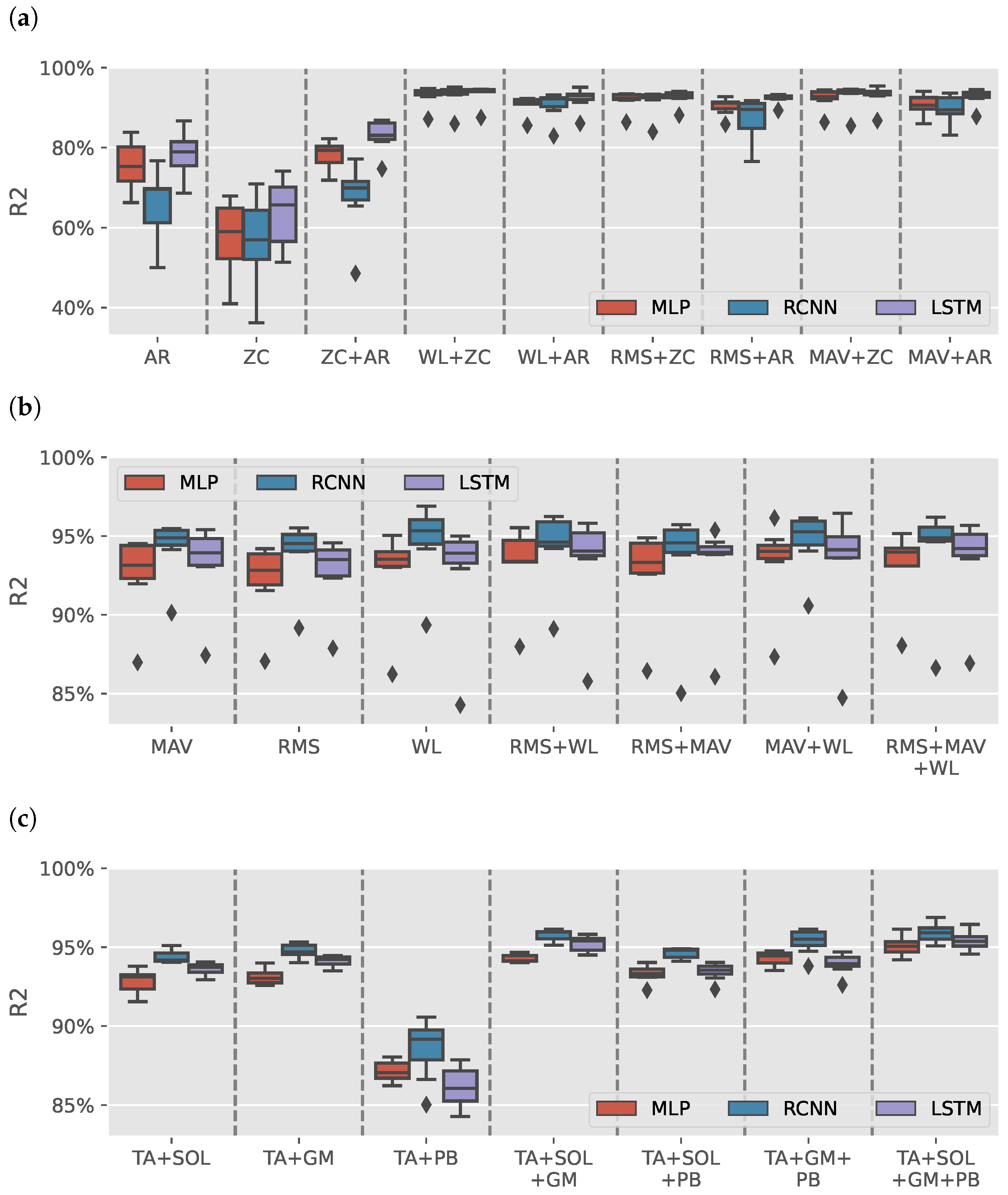
Figure 3a shows the results distribution of the models trained on AR or ZC features with a max of two features (due to space limitation). Each boxplot contains the results from 49 different intrasubject models. Models trained with either AR or ZC features only tended to have high variance in results depending on the muscles selected, DL model and volunteer with wide range from for RCNN (TA+GM AR) model trained on S3 to for LSTM (TA+SOL+GM+PB AR) model trained on S5. Combining the two features reduces the variance in data. It helped improve LSTM models, yet the results had less variance than the other trained models.
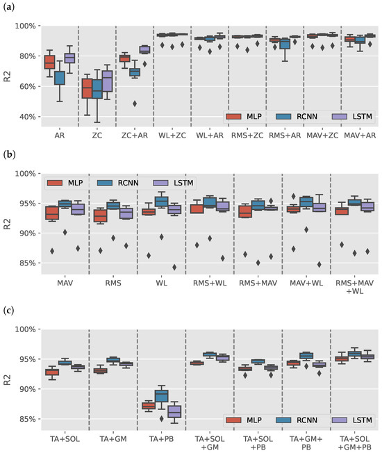
Figure 3.
sEMG intrasubject models results. (a) boxplots illustrate the distribution of values for models trained on various combinations of autoregressive model (AR) coefficients and zero crossing count (ZC) features. (b) illustrates the distribution of values for models trained on Signal Power features: root mean square (RMS), mean absolute value (MAV), and waveform length (WL). (c) shows the distribution of values for models for tibialis anterior (TA), soleus (SOL), gastrocnemius medialis (GM), and peroneus brevis (PB) muscles groups when using Signal Power features. The outliers observed in (b) are primarily attributed to the TA+PB muscle group, which exhibited lower estimation performance than other muscle groups.
Figure 3b shows the results of models trained using signal power features only (RMS, MAV, and WL). The figure has a single outlier for each model-features pair, which can also be found in Figure 3a in 17 out of 26 boxplots. Figure 3c shows the distribution of the results per muscle group using signal power features. All groups had an median greater than except for TA+PB models, which had lower estimation results, causing the outliers in Figure 3b.
Out of the 1302 trained models, the top three models were all sEMG models that achieved an average greater than and NRMSE average less than with a standard deviation less than , and , respectively. Table 2 shows the results of the top three sEMG models for each volunteer. The summary row shows the mean and standard deviation for each model and metric.
Table 2.
sEMG Intrasubject top three models’ results. The first model was a multi-layer perception (MLP) model trained by extracting the mean absolute value (MAV) and waveform length (WL) features from the tibialis anterior (TA), soleus (SOL), gastrocnemius medialis (GM), and peroneus brevis (PB) muscles. The second model was a recurrent convolutional neural network (RCNN) model trained by extracting the MAV and WL features from TA, GM, and PB muscles. The third model was an RCNN trained by extracting the WL feature only from TA, SOL, GM, and PB muscles.
RCNN (TA+GM+PB MAV+WL) model was superior to the MLP (TA+SOL+GM+PB MAV+WL) model. The RCNN (TA+SOL+GM+PB WL) model had higher intersubject variance than the other two models. However, its average values (: , NRMSE: ) were the best across all other sEMG models. LSTM (TA+SOL+GM+PB MAV+WL) was the only LSTM model able to fulfill the average criteria. However, the intersubject variance was high (: , NRMSE: ), suggesting that the model failed to learn the gait pattern of some volunteers properly, which makes it unlikely to work well for the intersubject model case.
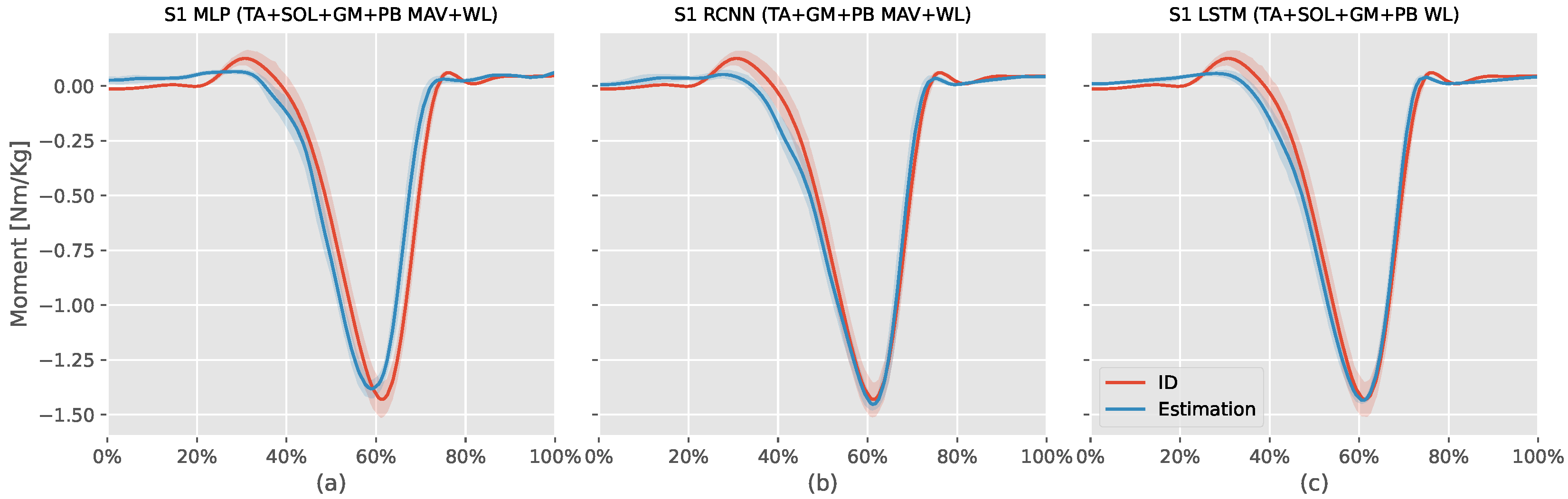
Figure 4 shows the ID moments against the three models mentioned above estimation for S1. The MLP model estimation (: , NRMSE: , RMSE: Nm/kg) had an offset value during the first swing phase, failed to estimate the positive dorsiflexor moment at the start and end of the stance phase, and estimated the stance phase moment earlier than the ID moments without being able to match the plantar flexor moment peak. The RCNN (TA+GM+PB MAV+WL) model estimation (: , NRMSE: , RMSE: Nm/kg) had better time synchronization with the ID was better than the MLP model, and was able to estimate the dorsiflexion moments at the start and end of the stance phase. However, it also had an offset during the first swing phase and could not estimate the plantar flexor moment peak.
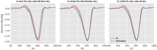
Figure 4.
This figure compares the estimated S1 (first volunteer) ankle moments from the inverse dynamic (ID) Equation (7) against intrasubject models (MLP, RCNN, LSTM) using the mean absolute value (MAV) and waveform length (WL) features extracted from tibialis anterior (TA), soleus (SOL), gastrocnemius medialis (GM), and peroneus brevis (PB) sEMG signals. The x-axis represents the normalized gait cycle, starting from the swing phase and ending with the subsequent swing phase. The y-axis shows the normalized ankle moment. Positive values indicate plantar flexion, while negative values indicate dorsiflexion. The shaded areas represent the standard deviation of the estimations across subjects.
Similar to the previous two models, the RCNN (TA+SOL+GM+PB WL) model estimation (: , NRMSE: , RMSE: Nm/kg) had offset during the first swing phase, and could not estimate the dorsiflexor moments at the start and end of the stance phase. However, this model could estimate the plantar flexor peak moment value and had better time synchronization with the ID results than the other two models.
RCNN (TA+GM+PB MAV+WL) and RCNN (TA+SOL+GM+PB WL) were the best intrasubject models trained on sEMG features. Therefore, these two models were used for training intersubject models.
3.1.2. DEMG Models
Figure 5a shows the results distribution of the DEMG models trained on AR or ZC features with a maximum of two features (due to space limitation). Like the sEMG models, models trained without power features tended to have low , and the models trained with ZC and either MAV or RMS could not fit variance in data. Figure 5b shows the models trained on power features alone. RCNN models trained using RMS + WL features had a wide range of depending on the selected muscles and subject. Similar to the sEMG models, the outlier in the results of the TA+PB muscles group is seen in Figure 5c.
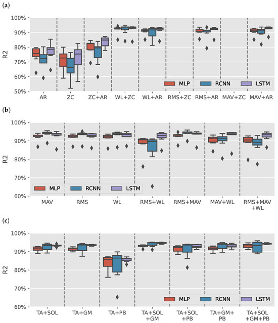
Figure 5.
DEMG intrasubject models results. (a) boxplots illustrate the distribution of values for models trained on various combinations of autoregressive model (AR) coefficients and zero crossing count (ZC) features. (b) illustrates the distribution of values for models trained on Signal Power features: root mean square (RMS), mean absolute value (MAV), and waveform length (WL). (c) shows the distribution of values for models for tibialis anterior (TA), soleus (SOL), gastrocnemius medialis (GM), and peroneus brevis (PB) muscles groups when using signal power features.
The best-performance DEMG model was RCNN (TA+SOL+GM+PB RMS+MAV) achieved (: , NRMSE: ). DEMG models had lower results than sEMG models. Therefore, they would not be used for the intersubject models.
3.2. Intersubject Model
Following the intrasubject models’ results, selected RCNN models were then trained for each volunteer using the leave-one-out approach. Table 3 shows the results of each trained intersubject model. The volunteers column in the table refers to the volunteers left out during the training and used for the evaluation. The summary row shows the mean and standard deviation of each intersubject model and metrics. RCNN (TA+SOL+GB+PB WL) intersubject models outperformed their corresponding RCNN (TA+GM+PB MAV+WL) models except for models evaluated on S1 and S3. Intersubject models were trained to learn unknown volunteer gait patterns, resulting in less accurate models than the intrasubject models; a similar observation was found in [16]. Unlike the intrasubject model cases, the model learns the volunteer’s walking patterns before testing them. The intersubject models’ results varied based on the volunteers’ data used for training, which resulted in a low average with high variance, especially for RCNN (TA+GM+PB MAV+WL) models. Both selected models’ architectures find difficulties estimating the S7 ankle moment.
Table 3.
Only 2 sEMG recurrent convolutional neural network (RCNN) models out of 1302 models were transferred for the intrasubject analysis. The first model was trained by extracting the waveform length (WL) features from the tibialis anterior (TA), soleus (SOL), gastrocnemius medialis (GM), and peroneus brevis (PB) muscles. The second model was trained by extracting the mean absolute value (MAV) and WL features from TA, GM, and PB muscles.
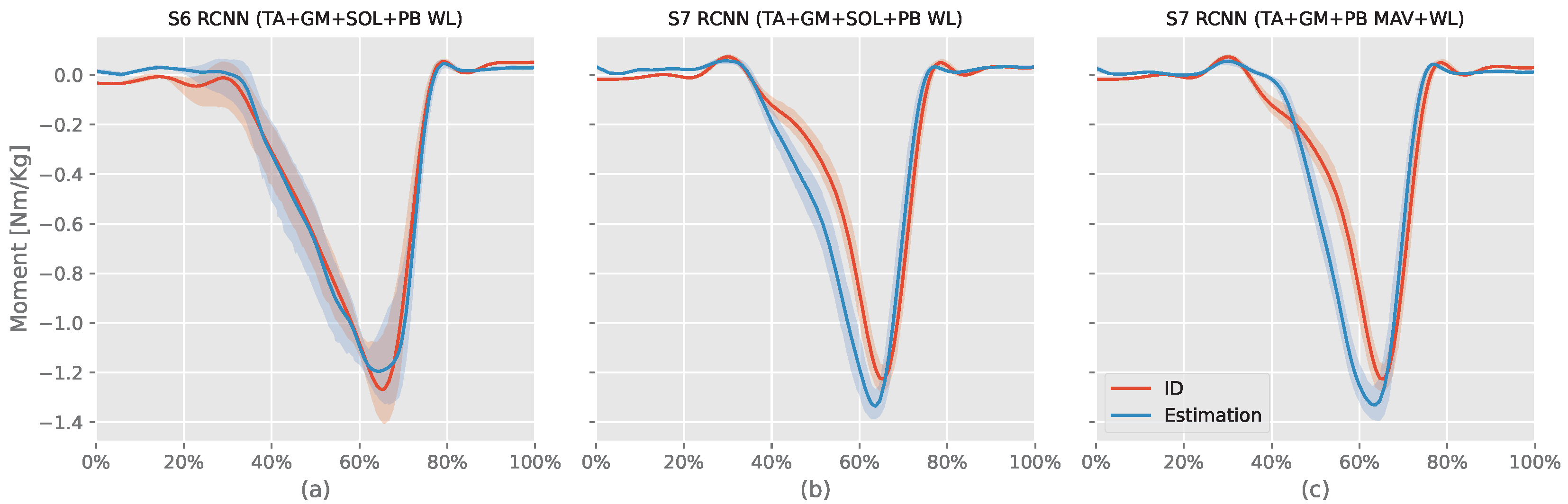
RCNN (TA+SOL+GM+PB WL) models evaluated on S5 and S6 had similar results with S6 (94.37%) greater than S5 () by , but S5 had NRMSE ) less than S6 NRMSE () by only. Looking at the RMSE, S6 (body mass = 69.5 kg) had RMSE ( Nm) less than S5 (body mass = kg) RMSE ( Nm). Figure 6 shows S6 RCNN (TA+SOL+GM+PB WL) intersubject model (best model) and both S7 intersubject models ID results against the estimated moment. The S6 model had a small offset during the first swing phase and could not estimate the peak plantar flexion moment value. However, it was able to synchronize the stance phase moment estimation with the ID moment and also estimate the dorsiflexion moment at the end of the stance phase.
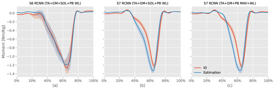
Figure 6.
This figure compares the three intersubject models against their corresponding ankle moments from the inverse dynamic (ID) Equation (7). The x-axis represents the normalized gait cycle, starting from the swing phase and ending with the subsequent swing phase. The y-axis shows the normalized ankle moment. Positive values indicate plantar flexion, while negative values indicate dorsiflexion. The shaded areas represent the standard deviation of the estimations across subjects. S6 and S7 refer to volunteers number 6 and 7, respectively, tibialis anterior (TA), soleus (SOL), gastrocnemius medialis (GM), and peroneus brevis (PB) muscles.
S7 ID planter moment increased between “ to of the record period”. At the same time, the RCNN (TA+GM+PB MAV+WL) model slowly decreased the dorsiflexion moment resulting in a gap between the ID moment and estimation. In contrast, the RCNN (TA+SOL+GM+PB WL) estimated this change. The ID planter moment slowly increased after until reaching the peak planter moment. In contrast, both RCNN models had rapid increases simultaneously, resulting in a gap between the ID moment and the model’s estimated moment during the first part of the stance phase. In summary, neither model can adapt to the volunteer moment’s rate of change. For the remaining part, both RCNN models’ moments were slightly ahead of the ID moment. They could both estimate the toe-off dorsiflexion moment.
4. Discussion
This research was conducted to analytically find a transferable deep learning (DL) model for ankle moment estimation by exploring 1302 different models, muscles, and feature combinations. Previous research focused on a single-model analysis [5,8,12,15]. Zhang et al. [8] trained the same MLP model, but used six different training scenarios resulting in six models per volunteer all having the same architecture. The best model in [8] for normal gait was an NMS model (RMSE: Nm/kg), which demonstrated poorer performance than the RCNN (TA+SOL+GM+PB WL) model (RMSE: Nm/kg). Siu et al. [11] trained four models per volunteer to estimate the ankle moment during standing, walking, running, and sprinting activities. On the other hand, Kim et al. [13] trained 33 MLP models for a classification task by changing the selected muscles for the model input. Compared to the previously mentioned studies, our study focused solely on normal walking activities but trained 1302 different intrasubject DL models to find suitable models, muscles, and feature combinations for the task. To the best of our knowledge, this is the first study that attempts to find a suitable combination of models, features, and muscle selection for the lower extremities moment estimation.
The architectures of the three selected models were designed to have a few layers and parameters to avoid overfitting the data and reduce computational costs for fast training and prediction. Indeed, the largest MLP model had 2609 trainable parameters, while the largest RCNN model and LSTM models had 2101 and 1865, respectively. The MLP, CNN, neural ODE, and LSTM models from [11] had 30,642, 156,264, and 32,306 trainable parameters, respectively. Comparing these parameter counts to our RCNN (TA+SOL+GM+PB WL) model, which had only 757 parameters, our best model had an intrasubject RMSE of Nm/kg, achieving similar performance to the LSTM model in [11] (RMSE: Nm/kg) with only of the total parameter count.
The study found that signal energy information features, such as WL, are sufficient for ankle moment estimation if the correct muscles are chosen, similar to the results found in [10] for sEMG-based models for hand classification. In contrast, signal frequency information features such as ZC and predictive model features such as AR coefficients make it hard to extract meaningful information to describe the moment. While most previous studies focused on the sEMG signals, we also explored the differentiated surface electromyography (DEMG) feature domains. We found that DEMG features result in low performance in the regression task.
Previous studies such as [5,8,11,12,15] predetermined muscles, and feature selection, but the selection combination is indeed an essential factor for model performance. Models trained on the wrong muscle group (TA+PB only) had low performance regarding the selected features and models’ architecture. The RCNN (TA+GM AR) and RCNN (TA+SOL+GM+PB AR) were models both trained on the same time-domain features but with different muscle selections; the former had a minimum of , while the latter scored a max of 96.56%. Two of the top three intersubject models and the best intrasubject models used all four targeted shank muscles in the study. Using more muscles showed better results as it helps the model learn synergistic actions from different sources, resulting in more varied information fed to the trained model, whereas using a set of power features might introduce highly correlated information rather than capturing the moment effectively.
MLP models tested in this study had high performance; however, they came with the cost of many parameters, such as needing to learn the time pattern and overfitting. On the other hand, LSTM is known for its use in the time-series models, but in this study, its performance was not better than the MLP models. Using RCNN allows the model to learn new features from existing ones before proceeding to the LSTM layers, resulting in better moment estimation.
Another factor that affects the DL models is the volunteer data. Models trained using sEMG features had distinct results from one volunteer to another. For example, the intersubject RCNN (TA+GM+Pb MAV+WL) model achieved an average score of when tested on S5 but only achieved when the model was tested on S7.
The nominated models for the intersubject model creation had RCNN architecture and WL features. Having the convolutional layer before the recurrent layers allowed the model to extract complex features from the extracted features. Both Intersubject models performed less than their related intrasubject models. A similar observation was reported in [16] when using DL to estimate knee kinematics and vertical GRF from IMU sensors. The best intersubject in this study was the RCNN (TA+SOL+GM+Pb WL) had achieved of , RMSE of , and NRMSE of using all selected muscles groups similar to the finding in the classification study in [13]. The best DEMG model RCNN (TA+SOL+GM+PB RMS+MAV) achieved (: , NRMSE: ) also used all muscles with the RCNN model architecture, but did not have the WL feature.
Mundt et al. [6] created MLP and LSTM models using simulated IMU data from a motion capture system, achieving an NRMSE of Nm/kg and Nm/kg, respectively. Moreira et al. [15] used volunteers’ anthropometrics and kinematics information from a motion capture system in a CNN model, achieving an of . While these models outperformed our RCNN (TA+SOL+GM+Pb WL) intersubject model (: , RMSE: Nm/kg), they used motion capture systems to generate the input data, which had limited walking space compared to the sEMG.
Despite achieving high results for the ankle moment estimation, the current study has some limitations:
- The results are based on OpenSim ID tools, and the ID results are assumed to be accurate.
- The walking space was relatively small, causing volunteers some difficulty in maintaining natural walking during the recording period.
- The study focused on normal gait and did not include other daily activities such as sitting, standing, and jumping.
- The study focused on training small DL models, and did not examine the impact of increasing model dimensions.
- The volunteers were asked to walk barefoot; wearing shoes or sports equipment can affect the activation level of the muscles [24,25].
- Only four muscles were used for building the models.
- The study was conducted on healthy males in their 20 s.
- Injured, aged, and amputee populations are the main targets for rehabilitation, yet the models were not tested on them.
5. Conclusions
This study investigated various combinations of deep learning (DL) models, sEMG features, and muscle selections to identify effective intrasubject models for estimating ankle moments during natural walking. The best-performing models and features were then transferred to train intersubject models. To mitigate overfitting and reduce computational costs, the models were trained with a limited number of parameters.
It was found that signal energy features were sufficient for intrasubject ankle moment estimation. However, frequency-based features (such as zero crossing count), predictive models, and signal differentiation posed challenges for small models due to the difficulty in learning such features. The top-performing sEMG and DEMG models utilized all the proposed muscles introduced in this study.
Finally, this study offers valuable insights into feature selection, muscle selection, and model architecture for intersubject DL models in ankle moment estimation. The proposed RCNN model, which employed waveform length (WL) features from all four shank muscles, demonstrated significant potential for practical applications, with only 757 parameters.
Author Contributions
Conceptualization, A.E.A.A., D.O. and M.H.; methodology, A.E.A.A.; software, A.E.A.A.; validation, A.E.A.A., D.O. and M.H.; formal analysis, A.E.A.A.; investigation, A.E.A.A.; resources, A.E.A.A. and M.H.; data curation, M.H.; writing—original draft preparation, A.E.A.A.; writing—review and editing, D.O. and M.H.; visualization, A.E.A.A.; supervision, M.H.; project administration, M.H.; funding acquisition, M.H. All authors have read and agreed to the published version of the manuscript.
Funding
This work was supported by JSPS KAKENHI Grant Number JP24K00841.
Institutional Review Board Statement
The study was conducted in accordance with the Declaration of Helsinki, and approved by the ethical committee of Tohoku University (protocol code 22A-3).
Informed Consent Statement
Informed consent was obtained from all subjects involved in the study.
Data Availability Statement
Data can be downloaded from 16 August 2024 on https://drive.google.com/drive/folders/1g4-s1zmAk3aFg4ilhfw60EnuLbNIdT6Z.
Conflicts of Interest
The authors declare no conflicts of interest.
Abbreviations
The following abbreviations are used in this manuscript:
| Autoregressive model | AR |
| Biceps femoris | BF |
| Convolutional neural network | CNN |
| Deep learning | DL |
| Differentiated electromyography | DEMG |
| Extensor digitorum longus | EDL |
| Flexor hallucis longus | FHL |
| Gastrocnemius lateral | GL |
| Gastrocnemius medialis | GM |
| Inertial measurement unit | IMU |
| Inverse Dynamic | ID |
| Long short-term memory | LSTM |
| Machine learning | ML |
| Mean absolute value | MAV |
| Mean squared error | MSE |
| Multi-layer perception | MLP |
| Neuromusculoskeletal | NMS |
| Normalized root square error | NRMSE |
| Ordinary differential equations | ODE |
| Peroneus brevis | PB |
| Coefficient of determination | |
| Rectus femoris | RF |
| Recurrent convolutional neural network | RCNN |
| Root mean square | RMS |
| Root mean square error | RMSE |
| Semitendinosus | ST |
| Soleus | SOL |
| Surface electromyography | sEMG |
| Tibialis anterior | TA |
| Vastus lateralis | VL |
| Vastus medialis | VM |
| Waveform length | WL |
| Zero crossing count | ZC |
References
- Morin, J.B.; Gimenez, P.; Edouard, P.; Arnal, P.; Jiménez-Reyes, P.; Samozino, P.; Brughelli, M.; Mendiguchia, J. Sprint acceleration mechanics: The major role of hamstrings in horizontal force production. Front. Physiol. 2015, 6, 404. [Google Scholar] [CrossRef]
- Chen, B.; Ma, H.; Qin, L.Y.; Gao, F.; Chan, K.M.; Law, S.W.; Qin, L.; Liao, W.H. Recent developments and challenges of lower extremity exoskeletons. J. Orthop. Transl. 2016, 5, 26–37. [Google Scholar] [CrossRef] [PubMed]
- Raković, M.; Savić, S.; Santos-Victor, J.; Nikolić, M.; Borovac, B. Human-inspired online path planning and biped walking realization in unknown environment. Front. Neurorobotics 2019, 13, 36. [Google Scholar] [CrossRef] [PubMed]
- Seel, T.; Raisch, J.; Schauer, T. IMU-based joint angle measurement for gait analysis. Sensors 2014, 14, 6891–6909. [Google Scholar] [CrossRef]
- Zhu, A.; Shen, H.; Shen, Z.; Li, Y.; Mao, H.; Zhang, X.; Cao, G. Prediction of Human Dynamic Ankle Moment Based on Surface Electromyography Signals. In Proceedings of the 2019 16th International Conference on Ubiquitous Robots (UR), Jeju, Republic of Korea, 24–27 June 2019; IEEE: Piscataway, NJ, USA, 2019; pp. 755–759. [Google Scholar]
- Mundt, M.; Thomsen, W.; Witter, T.; Koeppe, A.; David, S.; Bamer, F.; Potthast, W.; Markert, B. Prediction of lower limb joint angles and moments during gait using artificial neural networks. Med Biol. Eng. Comput. 2020, 58, 211–225. [Google Scholar] [CrossRef] [PubMed]
- Hayashibe, M.; Venture, G.; Ayusawa, K.; Nakamura, Y. Muscle strength and mass distribution identification toward subject-specific musculoskeletal modeling. In Proceedings of the 2011 IEEE/RSJ International Conference on Intelligent Robots and Systems, San Francisco, CA, USA, 25–30 September 2011; IEEE: Piscataway, NJ, USA, 2011; pp. 3701–3707. [Google Scholar]
- Zhang, L.; Li, Z.; Hu, Y.; Smith, C.; Farewik, E.M.G.; Wang, R. Ankle joint torque estimation using an EMG-driven neuromusculoskeletal model and an artificial neural network model. IEEE Trans. Autom. Sci. Eng. 2020, 18, 564–573. [Google Scholar] [CrossRef]
- Liu, G.; Zhang, L.; Han, B.; Zhang, T.; Wang, Z.; Wei, P. sEMG-based continuous estimation of knee joint angle using deep learning with convolutional neural network. In Proceedings of the 2019 IEEE 15th International Conference on Automation Science and Engineering (CASE), Vancouver, BC, Canada, 22–26 August 2019; IEEE: Piscataway, NJ, USA, 2019; pp. 140–145. [Google Scholar]
- Phinyomark, A.; Phukpattaranont, P.; Limsakul, C. Feature reduction and selection for EMG signal classification. Expert Syst. Appl. 2012, 39, 7420–7431. [Google Scholar] [CrossRef]
- Siu, H.C.; Sloboda, J.; McKindles, R.J.; Stirling, L.A. A neural network estimation of ankle torques from electromyography and accelerometry. IEEE Trans. Neural Syst. Rehabil. Eng. 2021, 29, 1624–1633. [Google Scholar] [CrossRef] [PubMed]
- Truong, M.T.N.; Ali, A.E.A.; Owaki, D.; Hayashibe, M. EMG-Based Estimation of Lower Limb Joint Angles and Moments Using Long Short-Term Memory Network. Sensors 2023, 23, 3331. [Google Scholar] [CrossRef]
- Kim, P.; Lee, J.; Jeong, J.; Shin, C.S. Deep learning-based identification algorithm for transitions between walking environments using electromyography signals only. IEEE Trans. Neural Syst. Rehabil. Eng. 2024, 32, 358–365. [Google Scholar] [CrossRef]
- Sakamoto, S.i.; Hutabarat, Y.; Owaki, D.; Hayashibe, M. Ground Reaction Force and Moment Estimation through EMG Sensing Using Long Short-Term Memory Network during Posture Coordination. Cyborg Bionic Syst. 2023, 4, 0016. [Google Scholar] [CrossRef] [PubMed]
- Moreira, L.; Figueiredo, J.; Vilas-Boas, J.P.; Santos, C.P. Kinematics, Speed, and Anthropometry-Based Ankle Joint Torque Estimation: A Deep Learning Regression Approach. Machines 2021, 9, 154. [Google Scholar] [CrossRef]
- Wouda, F.J.; Giuberti, M.; Bellusci, G.; Maartens, E.; Reenalda, J.; Van Beijnum, B.J.F.; Veltink, P.H. Estimation of vertical ground reaction forces and sagittal knee kinematics during running using three inertial sensors. Front. Physiol. 2018, 9, 218. [Google Scholar] [CrossRef] [PubMed]
- Ahmed, M.H.; Chai, J.; Shimoda, S.; Hayashibe, M. Synergy-Space Recurrent Neural Network for Transferable Forearm Motion Prediction from Residual Limb Motion. Sensors 2023, 23, 4188. [Google Scholar] [CrossRef]
- Hermens, H.J.; Freriks, B.; Disselhorst-Klug, C.; Rau, G. Development of recommendations for SEMG sensors and sensor placement procedures. J. Electromyogr. Kinesiol. 2000, 10, 361–374. [Google Scholar] [CrossRef] [PubMed]
- Delp, S.L.; Anderson, F.C.; Arnold, A.S.; Loan, P.; Habib, A.; John, C.T.; Guendelman, E.; Thelen, D.G. OpenSim: Open-source software to create and analyze dynamic simulations of movement. IEEE Trans. Biomed. Eng. 2007, 54, 1940–1950. [Google Scholar] [CrossRef] [PubMed]
- Seth, A.; Hicks, J.L.; Uchida, T.K.; Habib, A.; Dembia, C.L.; Dunne, J.J.; Ong, C.F.; DeMers, M.S.; Rajagopal, A.; Millard, M.; et al. OpenSim: Simulating musculoskeletal dynamics and neuromuscular control to study human and animal movement. PLoS Comput. Biol. 2018, 14, e1006223. [Google Scholar] [CrossRef] [PubMed]
- Phinyomark, A.; Quaine, F.; Charbonnier, S.; Serviere, C.; Tarpin-Bernard, F.; Laurillau, Y. Feature extraction of the first difference of EMG time series for EMG pattern recognition. Comput. Methods Programs Biomed. 2014, 117, 247–256. [Google Scholar] [CrossRef]
- Moisio, K.C.; Sumner, D.R.; Shott, S.; Hurwitz, D.E. Normalization of joint moments during gait: A comparison of two techniques. J. Biomech. 2003, 36, 599–603. [Google Scholar] [CrossRef]
- Englehart, K.; Hudgin, B.; Parker, P.A. A wavelet-based continuous classification scheme for multifunction myoelectric control. IEEE Trans. Biomed. Eng. 2001, 48, 302–311. [Google Scholar] [CrossRef]
- Sanchez-Gomez, R.; Becerro-de Bengoa-Vallejo, R.; Romero Morales, C.; Losa-Iglesias, M.E.; Castrillo de la Fuente, A.; López-López, D.; Díez Vega, I.; Calvo-Lobo, C. Muscle activity of the triceps surae with novel propulsion heel-lift orthotics in recreational runners. Orthop. J. Sport. Med. 2020, 8, 2325967120956914. [Google Scholar] [CrossRef] [PubMed]
- Sánchez-Gómez, R.; Romero-Morales, C.; Gómez-Carrión, Á.; Zaragoza-Garcia, I.; Martinez-Sebastian, C.; Ortuño-Soriano, I.; Gomez-Lara, A.; De la Cruz-Torres, B. Assessment of a New Lateral Cushioned Casting Orthosis: Effects on Peroneus Longus Muscle Electromyographic Activity During Running. Orthop. J. Sport. Med. 2021, 9, 23259671211059152. [Google Scholar] [CrossRef] [PubMed]

Disclaimer/Publisher’s Note: The statements, opinions and data contained in all publications are solely those of the individual author(s) and contributor(s) and not of MDPI and/or the editor(s). MDPI and/or the editor(s) disclaim responsibility for any injury to people or property resulting from any ideas, methods, instructions or products referred to in the content. |
© 2024 by the authors. Licensee MDPI, Basel, Switzerland. This article is an open access article distributed under the terms and conditions of the Creative Commons Attribution (CC BY) license (https://creativecommons.org/licenses/by/4.0/).