Article

Enhancing Marine Topography Mapping: A Geometrically Optimized Algorithm for Multibeam Echosounder Survey Efficiency and Accuracy

1
School of Computer Science and Cyber Engineering, Guangzhou University, Guangzhou 510006, China
2
School of Mathematics and Information Science, Guangzhou University, Guangzhou 510006, China
3
AI Thrust, The Hong Kong University of Science and Technology (Guangzhou), Guangzhou 511455, China
*
Authors to whom correspondence should be addressed.
Appl. Sci. 2024, 14(19), 8875; https://doi.org/10.3390/app14198875
Submission received: 14 August 2024 / Revised: 23 September 2024 / Accepted: 30 September 2024 / Published: 2 October 2024
(This article belongs to the Section Marine Science and Engineering)

Abstract

:
This research introduces a new multibeam survey line model that optimizes geometric relationships to improve the efficiency and accuracy of surveys over complex seabed topographies. Since existing multibeam echosounder systems have limitations in handling complex terrains, this study presents an advanced model to enhance data quality and operational efficiency. By strategically designing survey lines and optimizing coverage strategies, this paper achieves the optimal configuration of survey lines for secondary measurements in marine areas, ensuring high precision and reliability of measurement data. Experimental results show that the new model significantly outperforms existing technologies in terms of effective coverage area and measurement accuracy, with an average coverage rate of over 95%, higher than existing models, and a weighted average overlap rate of 3.18%, greatly improving the economic efficiency of measurements by reducing redundant coverage and minimizing operational costs. These findings confirm the advantages of the new model in practical applications and offer valuable technical support for advancing seabed mapping technology.

1. Introduction

Beam echosounder systems play a crucial role in marine topography mapping [1], utilizing the principles of sound wave propagation to measure seabed depth and topographical features, thereby obtaining precise data. These data are invaluable for understanding ocean changes, forecasting future trends [2], and formulating response strategies [3], and have significant practical implications for marine science research [4], seabed resource development [5], navigational safety, and environmental protection [6]. Compared to traditional single-beam echosounder technology, Multibeam Echosounder (MBES) systems offer the advantage of simultaneously transmitting and receiving multiple sound beams, covering a broader area of the seabed, significantly enhancing measurement efficiency and reducing data blind spots [7].
The core components of the MBES system include transmitters, receivers (transducers), signal processors, and high-precision navigation positioning systems [8], all of which are detailed in Figure 1. The system emits dozens to hundreds of sound beams perpendicularly to the ship’s course, covering a wide area of the seabed. The reflected signals from the seabed are precisely captured by the receivers and analyzed by the signal processor to calculate the depth values. The advantage of the multibeam system lies in its ability to provide continuous depth coverage, significantly enhancing mapping efficiency and accuracy. Particularly in dealing with complex seabed terrains, the system ensures high measurement precision and reliability through meticulous beam management and optimization [9].
Although modern sea areas have mostly been surveyed with single-beam or traditional multibeam echosounder systems, the continuous change in seabed topography and the limitations of previous measurements make it particularly important to design an efficient and accurate multibeam measurement method for those critical areas that undergo significant changes and require multiple surveys. Taking the South China Sea as an example, this region is not only one of the busiest shipping routes in the world, handling more than one-third of the global maritime cargo annually, but it is also rich in underwater oil and gas resources and biodiversity [10]. The economic and strategic importance of the South China Sea requires its seabed topography to be measured with high accuracy and updated frequently. However, traditional multibeam echosounding systems face significant challenges in dealing with complex terrain and the high costs of data collection and processing [11], which severely affect the accuracy and reliability of the measurements. In response to these challenges, our study proposes an innovative multibeam measurement model that leverages intelligent algorithms to generate optimized survey plans based on previous surveys of the seabed. This new approach significantly improves the accuracy and efficiency of measurements, especially in resource-rich deep-water areas, and has the potential for global impact [12]. This study aims to provide an efficient and accurate multibeam measurement solution for these critical sea areas by utilizing historical data to enhance the resurvey process.
Since the beginning of the 21st century, multibeam bathymetric technology has been extensively studied and applied [13]. These studies primarily focus on terrain tracking and data processing techniques, the design and implementation of signal processing systems, and the optimization of multibeam survey line layouts, thus advancing the standardization and regulation of multibeam bathymetry. The application areas of this technology continue to expand, covering deep-sea exploration, oceanic mapping, and seabed prospecting. However, despite the groundbreaking progress in multiple studies, practical application limitations exist. For instance, the semi-automatic seabed geological classification method based on multibeam data and maximum likelihood classification proposed by Parkinson, F., Douglas, K., and Li, Z. is innovative. However, it needs more extensive validation in various geological environments, which may limit its broader application [14].
Similarly, the marine habitat mapping study conducted by Hakim, A.M.M. and his team using a multibeam echosounder and underwater video observations in Tioman Marine Park offered new methods. However, it was limited to a single case study, potentially failing to capture variations across different marine habitats [15]. The study by Abubakari, A. and Poerbandono, examining the effectiveness of a vertical error budget model for a portable multibeam echosounder in a shallow water bathymetric survey, demonstrated significant improvements in measurement precision, yet its performance in deeper or more turbulent waters remains untested [16]. Additionally, the polar ocean multibeam survey line layout system designed and implemented by Wang Fengfan and Ma Yong, though adapted to extreme conditions, did not consider its adaptability in non-extreme environments or different seabed compositions [17]. Dong Yu’s discussion on applying MBES systems in marine channel measurement highlighted its importance and utility in channel mapping. However, the study did not explore the economic impacts of widespread implementation [18]. Finally, the comprehensive analysis of the current status and precision of seabed terrain detection and model development by Hao Ruijie, Wan Xiaoyun, and Sui Xiaohong, although providing an evaluation of the accuracy and efficiency of existing technology, also called for further innovation to enhance current techniques [19].
This study has developed a new set of multibeam echosounder algorithms and models, tailored to meet the seabed terrain measurement needs of various maritime areas. By deeply analyzing the mechanisms of sound wave propagation in seawater and their interactions with seabed topography, a depth measurement model based on spatial geometric relationships has been established to address the challenges of complex and variable seabed terrain. This research aims to enhance measurement efficiency and accuracy, providing crucial data support and technical assurance for seabed scientific research and resource exploration.
The main contributions of this study include the following:
  • A new multibeam echosounder model was developed utilizing geometric optimization techniques, significantly enhancing measurement accuracy and data integrity, particularly in complex seabed terrains.
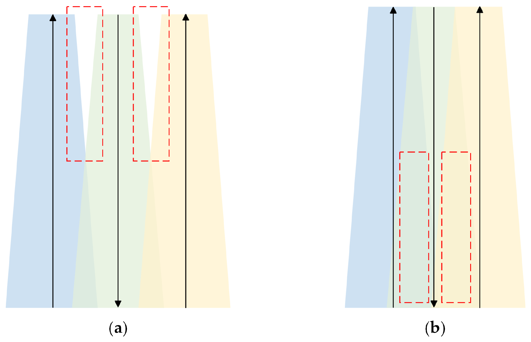
  • An optimized multibeam measurement algorithm was designed capable of dynamically adjusting survey line configurations in regions requiring frequent measurements, thus improving efficiency and reducing data overlap and resource wastage.
  • The performance of multibeam echosounding technology in practical applications was enhanced, providing critical support for marine science research and seabed resource exploration.

2. Research Content and Methodology

The primary focus of this research is to establish a multibeam survey line model optimized based on spatial geometric relationships aimed at enhancing the measurement effects and efficiency of multibeam depth sounding across various marine areas. In this chapter, Section 2.1 primarily discusses the accuracy standards of multibeam depth sounding systems, detailing the key parameters used during the measurement process. Section 2.2 elaborates on the methodology of this research, describing the applicability and principles of the two models discussed.

2.1. Coverage and Measurement Accuracy Standards

Traditional survey methods often use fixed grid patterns or simple parallel lines, which fail to adapt to the varying geometries of the seabed. This lack of adaptation often results in inefficiencies and potential data gaps. In contrast, our geometrically optimized approach dynamically adjusts survey lines to align closely with the seabed’s natural contours. By integrating real-time topographical data and strategically planning the orientations and spacings of survey lines, our method significantly enhances the accuracy and efficiency of seabed mapping. Unlike traditional techniques, our approach effectively addresses inefficiencies, optimizes coverage, and minimizes data redundancy. Such adaptability is crucial for navigating complex marine environments and ensuring thorough and efficient seabed surveys.
In practical marine exploration, the overlap rate is introduced as an evaluation metric to meet the requirements for cost-effective and efficient detection [20]. Figure 2 illustrates the geometric diagram of the overlap rate. The coverage width W of the multibeam echosounder swath varies with the transducer’s beam angle θ and the water depth D. If the survey lines are parallel and the seabed is flat, the overlap rate between adjacent swaths is given by: η = 1 d W where d is the distance between adjacent survey lines, and W is the swath coverage width. If η < 0 , it indicates gaps in coverage. To ensure convenience in measurement and data integrity, there should be an overlap of 10% to 20% between adjacent swaths [21].
Due to the significant variations in actual seabed topography, as shown in Figure 3. Using the average depth of a sea area to design survey line spacing while ensuring an average overlap rate that meets requirements can lead to gaps in coverage in shallower areas, affecting the quality of measurements. Conversely, using the shallowest depth in the area to determine survey line spacing ensures sufficient overlap in the shallowest parts. However, it leads to excessive overlap in deeper areas, creating redundant data and reducing measurement efficiency. Therefore, developing an efficient multibeam survey line model has significant practical importance.

2.2. Methodology

To address issues with the insufficient accuracy and low efficiency of survey routes in MBES systems, we have developed two types of multibeam survey line models based on real seabed topography to tackle these issues, respectively. The first model, a basic model, is designed for seabeds that are inclined planes, solving the problem of measurement inaccuracies. The second model, an optimized model, is suitable for complex real seabed scenarios, particularly for important sea areas that require frequent remeasurement, offering optimized survey line configurations to resolve issues of low efficiency in measurement routes. Built upon the foundation of the first model, the second model effectively utilizes both models developed in this research to perfectly address the current shortcomings in practical measurements, significantly enhancing measurement efficiency and accuracy.

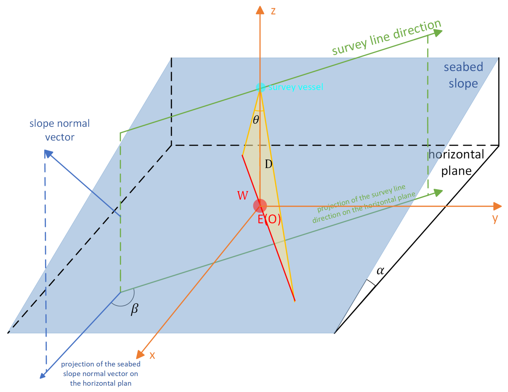
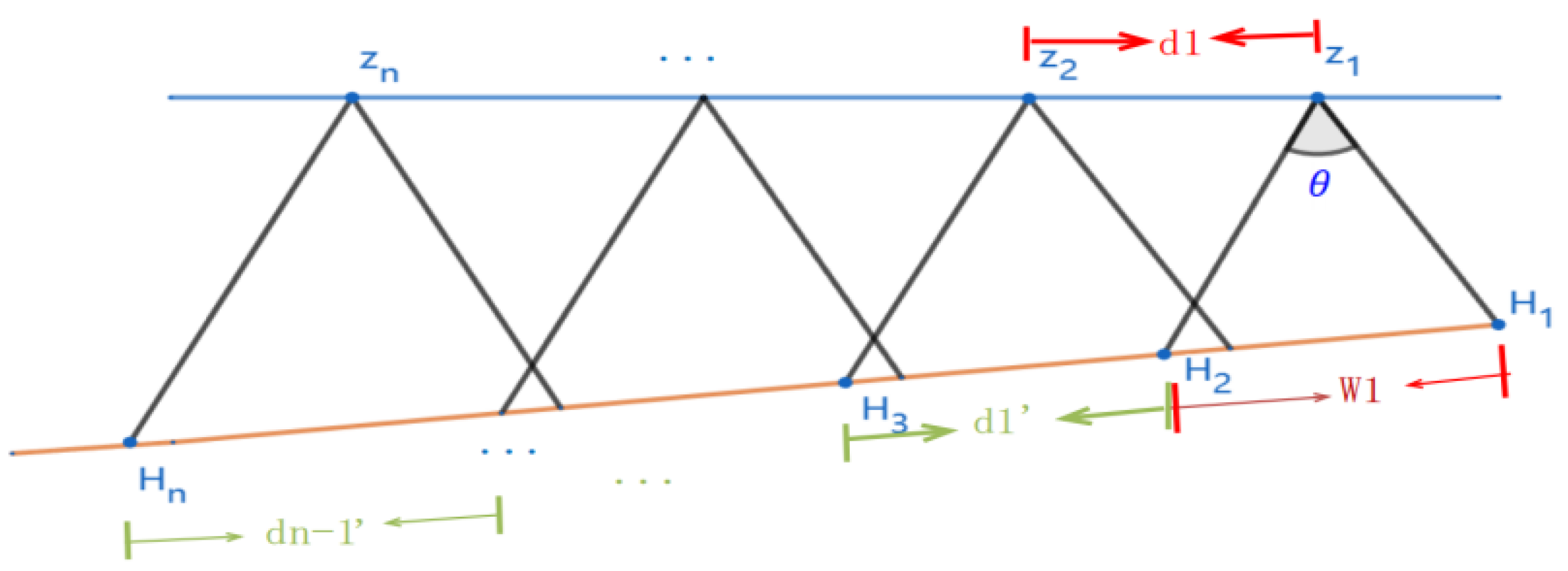
2.2.1. Precision Measurement Optimization Model

The Precision Measurement Optimization Model (PMOM) is designed to optimize measurement accuracy and efficiency. It is suitable for seabed topographies that are inclined planes, ensuring the efficient provision of high-precision data during the measurement process.
Applicable marine conditions: Within a water body where the seabed slope is a smooth inclined plane (assumed to be deeper in the west and shallower in the east), the east–west and north–south length of the sea area, the water depth D measured at the center of the sea area, the seabed slope α , and the opening angle θ of the multibeam transducer are known. The possible positions of the seabed slope relative to the horizontal plane are illustrated in Figure 4. Since the intersection of the seabed slope with the horizontal or sea surface may affect subsequent calculations of water depth, it is assumed that the projection of the seabed slope on the horizontal plane can cover the entire sea area, as shown in Figure 4b,c. Due to the unique topography of this sea area, high-precision measurements are necessary to obtain detailed information about the sea area.
For such regions, the PMOM can design a set of survey lines that fully cover the entire area to be measured, with adjacent stripes overlapping between 10% and 20%, fulfilling the requirement for the shortest total measurement length. This optimizes the model’s capability to address inaccuracies in measurements within such areas. The following are the implementation steps for the model.
Firstly, determining the survey line path is critical for achieving efficient measurement and minimizing the total length of the survey lines. The angle β formed by the projection of the survey line direction with the seabed slope’s normal on the horizontal plane can be controlled by fixing or changing β . According to the principle that the shortest distance between two points is a straight line, the total length of curved survey lines will inevitably be greater than that of straight lines. Therefore, to achieve high efficiency and accuracy in measurements, it is advisable to fix β for each survey line so that the lines are straight. As the water depth increases, both the coverage width W and the overlap rate η of the multibeam system increase. Therefore, the survey lines of this model start from the westernmost edge of the simulated maritime area as straight lines, laid out sequentially in the direction of increasing sea floor elevation. This arrangement maximizes the utilization rate of the coverage width in deep-sea areas, effectively reducing the total length of the survey lines.
The next crucial step is to maximize the coverage width W of the survey lines, as this directly impacts the required number of survey lines and the total length of the survey lines. To minimize the total survey line length, we derive the relationship between the coverage width W and the survey line direction β using the mathematical model and trigonometric functions illustrated in Figure 5 [22]. Calculating the optimal survey line direction β that maximizes the coverage width is essential. This step is critical because choosing the best β value affects the efficiency of coverage and determines the economy and accuracy of the entire measurement operation.
When the survey vessel is positioned at the center of the sea area, the relationship between the coverage width W and the angle β can be derived using the sine theorem and trigonometric functions. For a detailed derivation process, see Appendix A.1:
μ = arccos sin α sin β ( cos α sin β ) 2 + ( cos α cos β ) 2 + ( sin α sin β ) 2
W = D · sin θ 2 sin 180 θ 2 μ + D · sin θ 2 sin 180 θ 2 ( 180 μ )
Here, μ represents the angle between the center beam’s line and the line along which the coverage width W is measured. By applying Equations (1) and (2), we find that the survey line’s coverage width W is significantly influenced by β .
As shown in Figure 6, when β = 90 , the line representing the coverage width coincides precisely with the major axis of the ellipse, which is the longest segment within the ellipse [23]. Therefore, when considering the direction of the survey lines, choosing β = 90 can achieve the maximum coverage width, which is crucial for ensuring measurement efficiency at a given depth.
After determining the initial paths and directions of the survey lines, we proceed to the final solution phase. By employing trigonometric functions, we can precisely calculate the MBES system’s coverage width and overlap rate at various depths. In the design, we set a target overlap rate of 10%, aimed at maximizing the coverage area while reducing the total length of the survey lines, thereby ensuring the cost-effectiveness and efficiency of the measurement work.
Based on the requirement that the coverage area must meet or exceed the total area of the marine region, we used Formulas (1) and (2) to calculate various parameters, as shown in the survey line layout projection in Figure 7. Through these calculations, we have obtained the final results, which indicate that under the given sea area conditions, the optimal number of survey lines can be determined precisely through the following set of equations:
x = D x · tan θ 2 D x D 1 x = tan α D i D i + 1 d i = tan α a = 180 θ 2 α b = 180 θ a W i = D i · sin θ 2 1 sin a + 1 sin b d i = 0.9 W i d i = d i · sin 180 θ 2 sin 180 180 θ 2 α W 1 + i = 1 n d i h cos α
For more details, see Appendix A.2.
Using the PMOM model-designed survey lines, the most efficient and accurate measurement plan can be obtained for such marine areas.
Figure 7. This figure shows the projection of the survey line layout on the XOZ plane when β = 90 using the MBES system. The survey lines are set as straight lines to maximize the use of the multibeam transducer’s opening angle θ , thereby achieving the maximum coverage width W. In the diagram, D x represents the depth measured by each set of survey lines within the rectangular sea area, which helps to optimize the coverage width utilization in deep-sea areas. The survey lines extend parallel along the x-axis, and each line forms a straight line with the normal seabed slope on a plane at an angle α , ensuring continuity and efficiency of coverage. The points Q i indicate the intersection of the rightmost beam emitted by the survey vessel during the i-th measurement with the slope. At the same time, d 1 , d 2 , represent the distances between different survey lines, and d 1 , d 2 , represent the distances between Q i and Q i + 1 . By appropriately adjusting these distances, the coverage efficiency can be optimized, and the total length of the survey lines can be reduced.
Applsci 14 08875 g007

2.2.2. Complex Area Survey Line Optimization Model

The CASLOM model is fundamentally an optimized version of the PMOP model, incorporating PMOP’s algorithms to achieve efficient and high-precision measurements. It is specifically designed for complex, significant marine areas requiring repeated measurements. The primary aim of the CASLOM model is to develop the most efficient multibeam survey line configurations, optimizing the survey process to adapt effectively to challenging marine environments.
Applicable marine conditions: Within a specific real marine area, given that single-beam measurement data were used several years ago, and considering that marine conditions may have changed over the years and single-beam measurement data lack precision, it is necessary to optimize the general multibeam echosounder model. The goal is to achieve the optimal survey line layout so that the stripes formed along the survey lines cover the entire area to be measured as completely as possible, with minimal overlap between adjacent stripes and the shortest possible total length of the survey lines, in order to achieve the most efficient measurement results in practical surveys.
We collected single-beam survey data from 8 different sea areas recorded several years ago, each with a sampling area of 5 nautical miles in length (north–south) and 4 nautical miles in width (east–west). The data from the sixth sampling area were selected for demonstration. After data cleaning, the visualized results of the coordinates for this area are shown in Figure 8. Part of the single-beam bathymetric data for this sampling area is presented in Table A1 in Appendix B.1.
Using the CASLOM for such marine areas, it is possible to design a set of survey lines that maximize coverage and minimize overlap between lines, addressing the issue of inefficient survey routes. Below are the model’s implementation steps.
First, determine the optimization objectives. Based on the maritime conditions and the demands of on-site measurement, the following optimization goals have been defined:
Optimize min ( L total ) min ( S mea S mis )
where L total is the total length of the survey lines, S mea is the area covered by the survey lines, and S mis is the area missed in the measurements to enhance economic efficiency and measurement efficiency. The optimization problem is defined as follows:
Optimize min ( L total ) min ( S mea S mis ) max ( W ( x i , y i ) ) optimal navigation direction
Therefore, finding the maximum coverage width at each location within the maritime area is crucial. To meet the actual measurement needs, we need to consider both the determination of the navigation direction and the overlap rate. According to Model 1, we are starting the survey lines from the edge of the maritime area and arranging them to increase seabed elevation results in the maximum coverage width W.
The next step is to consider the optimal overlap rate between each survey line to maximize measurement efficiency, determining the minimum number of survey lines the MBES system needs to survey the area fully. Given that the overlap rate η is defined under the assumption of flat seabed topography, when the seabed slope is finely segmented, a small section of the slope can be approximated as a flat surface, thus maintaining the definition of η = 1 d / W . We adopt the straight-line approximation concept [24] for each coverage width segment W, where the overall optimal solution is composed of local optimal solutions.
We first determine the starting position of the survey ship. As shown in Figure 9, based on Model 1, a vertex H 1 of the curved marine area is selected as the starting coordinate because, at this point, the water is deeper, and both the coverage width and the overlap rate are greater.
Next, we calculate the data for each key point in the model based on geometric relationships. The coordinates of point Z 1 are calculated based on the multibeam’s opening angle θ , corresponding to point H 1 . From this, we can determine the equation of the line H 2 Z 1 and traverse all data points to find the H 2 point that satisfies this equation. If no data points satisfy the equation, we choose the point closest to the line H 2 Z 1 as H 2 .
Then, we calculate the length of the first coverage width W 1 , which is the Euclidean distance between H 1 and H 2 . Then, we determine the coordinates of the next point Z 2 , based on the position of Z 1 and d 1 . We then verify that all calculations meet the coverage width constraints and optimization goals to ensure the continuity and completeness of the multibeam coverage:
W 1 + i = 1 n d i H 1 H n η 20 %
Based on the steps outlined and Equation (5), the minimum number of multibeam transmissions required can be determined. For a detailed derivation of the formulas, see Appendix B.2.
Finally, by traversing all x values in the attachment, the minimum number of multibeam transmissions for different x values is determined. A survey line is formed by sequentially connecting each measurement point in the order of increasing x values, resulting in the projection of the optimal survey line array in the marine area. Then, we utilize the high-precision measurement model within the PMOM to complete subsequent surveys.

3. Results and Comparative Experiments

This chapter provides a detailed account of the experiments conducted in this study, demonstrating our approach’s efficiency and accuracy advantages, as well as its capability to handle complex seabed terrain data. Section 3.1 introduces the dataset and experimental environment used in this study; Section 3.2 presents the evaluation metrics for the experiments; Section 3.3 analyzes the experimental results and comparative experiments; and Section 3.4 summarizes the model and discusses its robustness.

3.1. Datasets and Experimental Environment

The dataset in this study contains depth and coordinate information of seabed topography. This dataset includes eight datasets, each collected from sampling areas in different sea regions, with each sampling area being a rectangular region of the same size (5 nautical miles ∗ 4 nautical miles). The dataset contains seabed coordinate data and seabed elevations within their respective areas. Table A1 in Appendix B.1 shows part of the data from the sixth sampling area. This dataset was obtained using single-beam echosounder models several years ago to illustrate seabed topography variations and features, serving as a critical reference for designing multibeam echosounder survey lines.
The datasets have been preprocessed to remove noise and anomalies, ensuring experiment accuracy. Each data group contains 250 rows and 200 columns, totaling 50,000 seabed coordinate data points. Each cell represents the seabed elevation at a point within the sampled area, expressed in negative meters, indicative of water depth. The coordinates are measured in units of 2 × 10 3 nautical miles. The data cover a range of seabed depths from shallow to deep, displaying complex underwater ridge features.
This study conducted experiments and comparative experiments within the sampled maritime area to validate the effectiveness of our model. Based on understanding the model used in this study, a series of assumptions were made about the experimental environment. These assumptions are fundamental to the model’s validity and impact its ability to solve practical problems. Assumptions include but are not limited to a constant transducer opening angle of 120°, the homogeneity of the seabed geology (not affecting the measuring beams’ reflection), the measuring equipment’s precision, and the margin of error in the data processing. Through these assumptions, we ensure the model’s applicability and the experimental results’ reliability.
The experimental environment for this study was based on Python 3.9, primarily utilizing NumPy 1.21.0 for numerical calculations, Pandas 1.3.0 for data analysis, Matplotlib 3.4.2 for data visualization, and SciPy 1.7.0 for scientific computation. All experiments were conducted on a Windows 10 Professional computer equipped with modern multi-core processors, ensuring processing efficiency and the reliability of the results.

3.2. Evaluation Metrics

The main evaluation criteria for the experiments include the following:
  • Effective Coverage Area: The total geographical area covered and effectively scanned by the survey lines, measured in square meters.
  • Coverage Rate [25]: The ratio of the effective coverage area to the total area of the survey region, serving as a key indicator of the model’s actual coverage within the marine area.
  • Total Survey Line Length: The sum of all survey line lengths, measured in meters, reflecting the efficiency of the survey model. The formula for calculating the average survey line length is:
    Average survey line length = Total line length Number of data sets
  • Weighted Average Overlap Rate: The weighted average value of the overlap rates between each survey line. It indicates the redundancy in the overlapping regions during the survey. The formula for calculating the weighted average overlap rate is:
    Weighted Average Overlap Rate = ( Overlap Rate × Overlap Region Length ) Total Survey Line Length

3.3. Experimental Results and Comparative Experiments

Since the CASLOM model already incorporates the algorithms and functions of the PMOP model, the experimental section focuses solely on evaluating and conducting comparative experiments on the CASLOM model, which is suited for complex marine environments.
Figure 10 illustrates the CASLOM model’s survey line results in the second, fourth, and sixth sampling areas of the marine region, demonstrating how the survey lines curve in response to the complex variations in the seabed terrain. The lines are arranged at certain intervals to ensure comprehensive area coverage while avoiding unnecessary resource waste. There is some overlap between the survey lines, with the overlap rate kept below 20%, ensuring continuity and redundancy of the survey data, preventing omissions, and improving measurement accuracy.
Table 1 displays the effects of survey line design by the CASLOM model across eight sampling areas in the marine region. Data from four key performance indicators show how our model performs across all datasets.
To comprehensively evaluate the application potential of our method in bathymetric surveying technology, we conducted a comparative analysis with three current cutting-edge academic research models.
Tannaz H. Mohammadloo and others proposed the Multibeam Echosounder Measurement Uncertainty Prediction Model (AMUST) [26], which uses statistical methods to predict measurement uncertainties, thereby improving the reliability of measurement data. Zhou, Chen, and Wang discussed the Dual Robust Strategy (DRS) for removing outliers in multibeam echosounding to enhance seabed terrain quality estimation [27], using advanced processing techniques to enhance the robustness and accuracy of data processing. Wojciech Maleika proposed the Local Polynomial Interpolation Optimization Method (LPIOM) [28], which improves the precision of terrain model generation by applying local polynomial interpolation techniques.
In addition, this experiment used a baseline model as the most basic control. This method uses a very basic multibeam echosounder system configuration, with evenly spaced survey lines and an interval between each line fixed at 700 m. In the baseline model, the survey vessel measures along the longer side of the sampling area as the survey line direction to reduce the number of turns.
We conducted experiments with these four models alongside our own using all data from the dataset, designing survey lines to determine the effective coverage area and total length of survey lines for each model. We then compared the performance metrics across the models. Table 2 displays the average results of comparative experiments conducted across eight datasets.
Our model achieves an effective coverage area of 1.1897 × 10 8 m2, with a coverage rate as high as 94.98%, the highest among all models. Additionally, our model is highly efficient regarding total survey line length, requiring only 474,662 m, which is shorter than any other model. In terms of the weighted average overlap rate, our model is only 3.18%, significantly lower than other models, indicating a notable advantage in avoiding measurement overlap.
Overall, the experimental results shown in Table 2 indicate that, when comparing our model’s performance with other multibeam echosounder models in unknown and complex marine environments, our model demonstrates significant advantages in several key performance metrics, showcasing its efficiency and reliability in marine surveys.

3.4. Model Robustness Analysis

By deriving the model, it can be seen that the depth of the sea area affects the coverage width and overlap rate of both PMOM and CASLOM, thereby influencing the measurement effect. Therefore, we conducted a robustness analysis on the two measurement models by changing the original dataset’s seabed depth to verify the models’ sensitivity and adaptability to changes in environmental variables.
For our robustness analysis experiment, we meticulously selected the second dataset as the control data. We then systematically adjusted the entire seabed elevation data within this sampling area by −300 m, −150 m, +150 m, and +300 m, creating four distinct sets of experimental data. This process allowed us to observe the models’ responses to varying environmental conditions. The results of this experiment are presented in Table 3.
We observed that the model demonstrates the highest coverage efficiency, lowest overlap rate, and best data integrity within the moderate water depth range (elevation from −550 m to −250 m). Although the overlap rate increases and data integrity slightly decreases under extreme water depth conditions (elevation of −700 m), the model maintains efficient and reliable performance across most water depths.

4. Discussion

Through the analysis of comparative experimental data, our model demonstrates superior performance across multiple key indicators, showcasing its unique design advantages and optimization methods. Firstly, our model employs intelligent algorithms to optimize survey line layout, allowing the lines to adapt to the seabed terrain’s complex variations dynamically, ensuring higher coverage efficiency and measurement accuracy. Our model achieves an effective coverage area of 1.1897 × 10 8 m2, significantly surpassing other models. Although the AMUST model enhances the reliability of measurement data, its effective coverage area is relatively smaller. Secondly, our model significantly reduces the total survey line length to only 474,662 m through refined algorithm optimization, demonstrating higher economic efficiency.
In contrast, while the LPIOM model improves the precision of terrain model generation, it may lose some key terrain features when dealing with complex topography. Our optimization method expands the coverage area and accuracy and reduces overlap rates, enhancing data integrity and measurement efficiency. These characteristics enable our model to complete measurements more efficiently and economically in practical applications.
Our model demonstrated significant advantages in the robustness analysis, particularly regarding adaptability and reliability under different water depth conditions. By altering the seabed depth of the original dataset, we validated the model’s sensitivity and adaptability to various environmental variable changes. The analysis results indicate that our model performs well under various elevation change conditions. When the elevation ranges from −550 to −250 m, our model exhibits optimal coverage efficiency and the lowest overlap rate, with an average overlap rate of only 7.51%. This indicates that our model can perform measurements most effectively under moderate water depth conditions while maintaining high measurement accuracy and data integrity.
Our model performs well in many respects, yet it has limitations. It is designed for marine areas that have previously been surveyed and now require remeasurement due to changes over time or new needs. These areas typically have existing single-beam survey data. Thus, the optimization algorithm partly depends on prior knowledge of seabed characteristics, which may limit its application in uncharted or sparsely mapped terrains. Additionally, while the model is generally stable, it may encounter challenges in highly complex terrains or where substantial data noise is present.
Future research could focus on improving the model’s adaptability and accuracy in unknown or data-sparse regions by incorporating machine learning-based predictive algorithms that can infer seabed features from minimal initial data. Another potential area for development involves integrating a comprehensive path-planning system, combining software and hardware, which uses real-time seabed topography data from current scans to adjust survey routes dynamically. This system could optimize survey efficiency, reduce reliance on prior data, and ensure the model’s robustness across various complex marine environments. These advancements would contribute to more flexible and precise seabed mapping techniques in increasingly challenging terrains.

5. Conclusions

To summarize, our model demonstrates significant improvements in efficiency and accuracy in multibeam echosounding measurements through advanced optimization techniques and intelligent algorithms. The model dynamically adapts to complex seabed terrain, ensuring extensive coverage and minimal survey line overlap, achieving an effective coverage area of 1.1897 × 10⁸ m2 with a total survey line length of only 434,662 m. This high efficiency is maintained alongside excellent accuracy, and data integrity remains strong even under varying environmental conditions. Our model is rated high in robustness and generalization ability, proving its reliability and adaptability in diverse marine environments.
Furthermore, robustness analysis indicates that our model maintains high performance under varying depth and slope conditions, showcasing its versatility and practicality in real-world applications. Despite some limitations in extreme conditions, the overall performance significantly surpasses existing models, highlighting the potential of our model to enhance the accuracy, efficiency, and reliability of marine measurements. Continuous optimization and field testing will further strengthen these findings and extend the model’s applicability to a broader range of marine measurement scenarios.

Author Contributions

All authors made significant contributions to the conceptualization and design of the study. The field experiments and data collection were conducted by Y.L. under the supervision of Y.Z.; J.X. provided assistance with the modeling. The manuscript was primarily written by Y.L. and critically reviewed and edited by H.L. and Y.Z. All authors have read and agreed to the published version of the manuscript.

Funding

This work is supported by the National Natural Science Foundation of China (No. 12250410247) and the Ministry of Science and Technology of China (No. WGXZ2023054L).

Institutional Review Board Statement

Not applicable.

Informed Consent Statement

Not applicable.

Data Availability Statement

Data is contained within the article.

Acknowledgments

The authors would like to thank Zhong Yubin for his support and guidance in this research.

Conflicts of Interest

The authors declare no conflicts of interest.

Appendix A. Derivation of the Precision Measurement Optimization Model

Appendix A.1. Derivation of Equations (1) and (2)

To determine the relationship between the coverage width W and the orientation angle β , selecting the optimal direction of the survey line that maximizes the detection coverage at the center of the marine area is crucial. This process requires the use of a Cartesian coordinate system. By deriving the plane equations for the seabed slope A and the multibeam plane B when the ship is at the center (distance zero), the line l 1 representing the coverage width W can be established. From there, using the sine theorem, the coverage width W is calculated.
Definition A1. 
General Equation of a Plane in Space [29]. Any plane in space can be defined by a point M 0 ( x 0 , y 0 , z 0 ) on the plane and its orientation vectors a = ( X 1 , Y 1 , Z 1 ) and b = ( X 2 , Y 2 , Z 2 ) . Thus, any plane can be represented by the following equation:
x x 0 y y 0 z z 0 X 1 Y 1 Z 1 X 2 Y 2 Z 2 = 0
The above results are expanded in:
A x + B y + C z + D = 0
where
A = Y 1 Z 1 Y 2 Z 2 , B = Z 1 X 1 Z 2 X 2 , C = X 1 Y 1 X 2 Y 2 , D = x 0 y 0 z 0 X 1 Y 1 Z 1 X 2 Y 2 Z 2
Since vectors a and b are not collinear, A, B, and C are not all zero, indicating that any plane in space can be represented by a linear equation in x, y, and z.
Definition A2. 
If a point M 0 ( x 0 , y 0 , z 0 ) and a non-zero vector n = ( A , B , C ) are given in space, then the plane passing through M 0 and perpendicular to n is uniquely determined. The vector n , being perpendicular to the plane, is called the normal vector of the plane. Thus, the point-normal form of the equation of the plane [30] can be expressed as:
A ( x x 0 ) + B ( y y 0 ) + C ( z z 0 ) = 0
Theorem A1. 
The direction vector of the line of intersection of two planes A and B can be determined by the cross product of their normal vectors [31].
Proof of Theorem A1. 
Consider two planes A and B with equations:
A : A 1 x + B 1 y + C 1 z + D 1 = 0 , B : A 2 x + B 2 y + C 2 z + D 2 = 0 .
In the Cartesian coordinate system, the normal vectors of the planes are n 1 = ( A 1 , B 1 , C 1 ) and n 2 = ( A 2 , B 2 , C 2 ) . The direction vector v of their line of intersection can be computed as:
v = n 1 × n 2 = B 1 C 1 B 2 C 2 , C 1 A 1 C 2 A 2 , A 1 B 1 A 2 B 2
First, the equations for the seabed slope plane A, the multibeam plane B, and the survey line direction plane C are determined. As shown in Figure 5, after establishing the Cartesian coordinate system, the projection diagrams of these three planes are obtained:
Figure A1. This figure depicts the relationships between normal directions and angles on different spatial planes. (a) illustrates the angular relationships on the X O Z plane. In this diagram, n 1 represents the normal of this plane, making an angle α with the z-axis. (b) shows the angular relationships on the X O Y plane. Here, n 2 represents the normal of this plane, forming an angle β with the x-axis. (c) illustrates the projection of plane C on the X O Y plane with n 2 , while n 3 is the normal vector of plane C passing through the origin.
Applsci 14 08875 g0a1
As shown in Figure A1a, n 1 is the normal vector of the seabed slope A, where n 1 = ( sin α , 0 , cos α ) . Since the seabed slope A passes through the origin, the point-normal form of the equation for plane A is given by:
x · sin α + z · cos α = 0
As illustrated in Figure A1b, n 2 is the normal vector of plane B, which passes through the origin and lies on the X O Y plane. The direction of the survey line is perpendicular to plane B; hence, the angle β between n 2 and the x-axis is given by n 2 = ( cos β , sin β , 0 ) . Since plane B passes through the origin, the point-normal form of the equation for plane B is:
x · cos β + y · sin β = 0
As depicted in Figure A1c, the projection of plane C onto the X O Y plane is represented by n 2 , and n 3 is the normal vector of plane C passing through the origin. It follows that n 3 = ( sin β , cos β , 0 ) . Since plane C passes through the origin, the point-normal form of the equation for plane C is:
x sin β y cos β = 0
To find the line of intersection l 1 between plane A and plane B, consider their normal vectors:
n 1 = ( sin α , 0 , cos α ) , n 2 = ( cos β , sin β , 0 ) .
According to Theorem A1, the direction vector w of the line of intersection l 1 is given by the cross product of the normal vectors of planes A and B:
w = ( cos α sin β , cos α cos β , sin α sin β ) .
Subsequently, the coverage distance at the central point of the marine area is determined. Figure A2 illustrates the triangle P Q H formed by the multibeam echosounder from the survey ship at the center of the marine area and the seabed slope.
Figure A2. This figure illustrates the triangle P Q H formed by the multibeam echosounder from the survey ship at the center of the marine area and the seabed slope. P E is aligned along the z-axis, and the length of H Q represents the coverage width W. The opening angle of the multibeam transducer is given by Q P H = θ = 120 and E P H = θ / 2 = 60 , where e i = ( 0 , 0 , 1 ) and D = P E = 120 m.
Applsci 14 08875 g0a2
Given the vectors e 1 = ( 0 , 0 , 1 ) and w , the angle μ , which is the angle between E H and P E , is computed as follows:
cos μ = e 1 · w | e 1 | · | w | = sin α sin β ( cos α sin β ) 2 + ( cos α cos β ) 2 + ( sin α sin β ) 2
Therefore, the angle μ is given by:
μ = arccos sin α sin β ( cos α sin β ) 2 + ( cos α cos β ) 2 + ( sin α sin β ) 2
Based on the sine rule, we obtain:
| E H | = D · sin θ 2 sin 180 θ 2 μ
| E Q | = D · sin θ 2 sin 180 θ 2 ( 180 μ )
Therefore, the coverage width W = | E H | + | E Q | is given by:
W = D · sin θ 2 sin 180 θ 2 μ + D · sin θ 2 sin 180 θ 2 ( 180 μ )
Thus, Equations (1) and (2) have been proven, establishing the relationship between W and β .

Appendix A.2. Derivation of Equation (3)

To determine the optimal number of survey lines, as shown in Figure 7, set parameters a and b, which are the acute angles between the leftmost and rightmost multibeam survey lines and the seabed slope, respectively. First, determine the length x. According to the tangent theorem, we have:
tan θ 2 = x D x
Next, determine the length D 1 . According to the tangent theorem, we have:
tan α = D x D 1 x
Subsequently, determine the expression for d i . Since the actual measurement must meet an overlap rate of 10–20%, and when the overlap rate is minimized, the multibeam coverage area is maximized, resulting in the shortest survey line length and the most efficient measurement. Therefore, we set the overlap rate at 10%:
1 d i W i = 0.1
Since the beams need to cover the entire plane, i.e., the coverage area must be greater than or equal to the area of the sea region, it must satisfy:
W 1 + i = 1 n d i h cos α
Following this, we determine the expression for the coverage width W i . According to the sine rule, we have:
W i = D i · sin θ 2 1 sin a + 1 sin b
Finally, determine the expression for d i . According to the angle relationships in Figure 7, we have:
d i = d i sin 180 180 θ 2 α · sin 180 θ 2
Thus, Equation (3) is proved, which allows us to determine the optimal number of survey lines under the given conditions of the marine area.

Appendix B. Derivation of the Complex Marine Area Survey Line Optimization Model

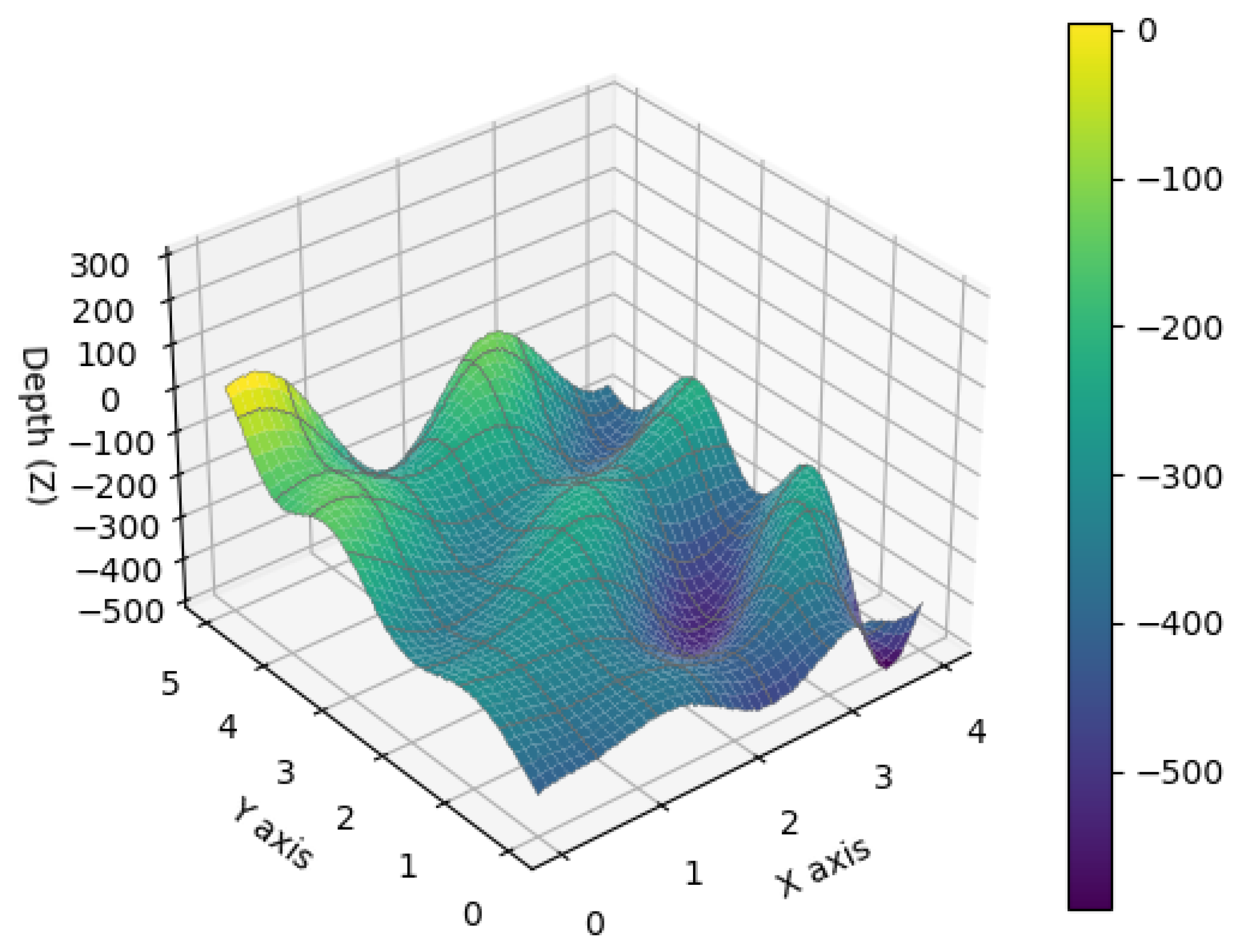
Appendix B.1. Seabed Coordinate Data of the Marine Area

Table A1 displays part of the data from the sixth sampling area among the eight different sea area sampling zones. This table only displays the sea depth from the sea level coordinates ranging from (0, 0) to (10, 7) within the sampling area, comprising a total of 10 × 8 coordinate points.
Table A1. The first row of the table represents the horizontal coordinates of the seabed (from west to east), the first column represents the vertical coordinates (from south to north), and the remaining data represent the elevation of the seabed.
1234567
1−419.519−418.317−414.532−411.712−411.083−411.856−410.857
2−416.148−415.537−411.993−410.414−410.186−409.167−410.403
3−411.267−410.704−408.855−409.708−406.032−409.945−407.646
4−407.436−408.972−405.738−407.693−404.474−402.182−402.857
5−407.433−401.795−402.713−402.887−402.613−400.351−397.257
6−401.516−402.432−398.618−400.311−401.117−400.850−396.713
7−399.641−398.642−398.293−404.488−395.189−395.352−397.226
8−397.070−396.186−394.851−390.699−391.679−396.517−394.961
9−392.621−395.804−394.211−394.150−390.677−387.531−392.386
10−390.828−390.449−389.131−388.218−389.258−388.942−387.434
The units of the horizontal and vertical coordinates in the table are 2 × 10 2 nautical miles, and the unit of water depth is meters. One nautical mile = 1852 m.

Appendix B.2. Derivation of Model 2 in Section 2.2.2

First, determine the starting position of the survey vessel. According to the analysis of Model 1 in Section 2.2.1, as the water depth increases, the coverage width W becomes larger, and the overlap rate η also increases. By traversing the four boundary points of the rectangular curved surface area, as shown in Figure 9, the point H 1 ( 0 , y 0 , z 0 ) is selected as the starting coordinate for the survey vessel.
Secondly, the coordinates of each key point in the model are determined based on geometric relationships. The coordinates of Z 1 are ( 0 , y 1 , 0 ) . Given that the multibeam angle is θ , we know that:
y 0 y 1 z 0 = tan 90 θ 2
Since H 2 Z 1 and Z 1 H 1 are symmetric about the angle bisector of the multibeam survey line, the equation of the line H 2 Z 1 is:
z = tan 90 θ 2 · ( y y 1 )
Since the line H 2 Z 1 must intersect with the intersection line of the slope surface and the multibeam plane, denote this intersection point as H 2 . By substituting all the data points from Table 1 into the line equation of H 2 Z 1 , if a data point satisfies the equation, it is H 2 . If no data points in Table 1 satisfy the line equation, choose the point on the intersection line of the multibeam plane that is closest to the line H 2 Z 1 as H 2 , denoted as H 2 ( 0 , y 1 , z 1 ) .
Using the concept of approximating curves with straight lines, the length of W 1 is the Euclidean distance between points H 1 and H 2 :
W 1 = ( y 1 y 0 ) 2 + ( z 1 z 0 ) 2
It is easy to see that the coordinates of Z 2 are ( 0 , y 2 , 0 ) , which can be expressed as ( 0 , y 1 + d 1 , 0 ) .
Finally, we need to satisfy the coverage width constraint. As shown in the optimization objective (4), the sum of W 1 and d i should be as large as possible to ensure the measurement model covers the entire seabed area, minimizing the uncovered area, and the overlap rate should be less than or equal to 20%. Here, d i is the difference between the coverage width W i + 1 and the overlap portion between W i + 1 and W i , i.e., d i = W i + 1 W i η i . The specific coordinates of H n can be obtained from Table 1.
W 1 + i = 1 n d i H 1 H n η i 20 %
The optimal number of survey lines can be determined by optimizing the above equations.
Finally, by iterating through all the x values in Table 1 as the x-coordinate of H 1 , and solving the equations, we can sequentially connect each survey point in increasing order of x values to form a survey line. The resulting optimal survey line group projection in the sea area will meet the problem’s requirements. Thus, the derivation of CASLOM in Section 2.2.2 is complete.

References

  1. Casalbore, D. Multibeam Echosounder. In Remote Sensing for Characterization of Geohazards and Natural Resources; Springer International Publishing: Cham, Switzerland, 2024; pp. 159–169. [Google Scholar]
  2. Abbot, P.; Dyer, I. Sonar Performance Predictions Incorporating Environmental Variability. In Impact of Littoral Environmental Variability on Acoustic Predictions and Sonar Performance; Springer: Dordrecht, The Netherlands, 2002; pp. 611–618. [Google Scholar]
  3. Swain, J.; Umesh, P.A.; Harikrishnan, M. Role of Oceanography in Naval Defence. Indian J. Geo-Mar. Sci. 2010, 39, 631–645. [Google Scholar]
  4. Williamson, B.J.; Blondel, P.; Williamson, L.D.; Scott, B.E. Application of a Multibeam Echosounder to Document Changes in Animal Movement and Behaviour around a Tidal Turbine Structure. ICES J. Mar. Sci. 2021, 78, 1253–1266. [Google Scholar] [CrossRef]
  5. Trenkel, V.M.; Mazauric, V.; Berger, L. The New Fisheries Multibeam Echosounder ME70: Description and Expected Contribution to Fisheries Research. ICES J. Mar. Sci. 2008, 65, 645–655. [Google Scholar] [CrossRef]
  6. Brown, C.J.; Blondel, P. Developments in the Application of Multibeam Sonar Backscatter for Seafloor Habitat Mapping. Appl. Acoust. 2009, 70, 1242–1247. [Google Scholar] [CrossRef]
  7. Pratomo, D.G.; Saputro, I. Comparative Analysis of Singlebeam and Multibeam Echosounder Bathymetric Data. Proc. Iop Conf. Ser. Mater. Sci. Eng. 2021, 1052, 012015. [Google Scholar]
  8. Hughes Clarke, J.E. Multibeam Echosounders. Submar. Geomorphol. 2018, 25, 25–41. [Google Scholar]
  9. Maleika, W. Development of a Method for the Estimation of Multibeam Echosounder Measurement Accuracy. Prz. Elektrotechniczny 2012, 2, 4. [Google Scholar]
  10. Singh, N.K.; Morgan, R. Blue Stream Survey: Deepwater Challenge. In Proceedings of the Offshore Technology Conference, OTC, Houston, TX, USA, 30 April–3 May 2001. OTC-13156-MS. [Google Scholar]
  11. Zhu, W.L.; Zhong, K.; Li, Y.C.; Xu, Q.; Fang, D.Y. Characteristics of Hydrocarbon Accumulation and Exploration Potential of the Northern South China Sea Deepwater Basins. Chin. Sci. Bull. 2012, 57, 3121–3129. [Google Scholar] [CrossRef]
  12. Rahman, C.; Tsamenyi, M. A Strategic Perspective on Security and Naval Issues in the South China Sea. In Maritime Issues in the South China Sea; Routledge: London, UK, 2013; pp. 35–53. [Google Scholar]
  13. Ferreira, I.O.; Andrade, L.C.; Teixeira, V.G.; Santos, F.C.M. State of art of bathymetric surveys. Bol. Ciências Geodésicas 2022, 28, e2022002. [Google Scholar] [CrossRef]
  14. Parkinson, F.; Douglas, K.; Li, Z. A Generalized Semiautomated Method for Seabed Geology Classification Using Multibeam Data and Maximum Likelihood Classification. J. Coast. Res. 2024, 40, 1–16. [Google Scholar] [CrossRef]
  15. Hakim, A.M.M.; Che, R.H.; Md, N.S.; Said, M.S.M.; Razali, R. Marine Habitat Mapping using Multibeam Echosounder Survey and Underwater Video Observations: A Case Study from Tioman Marine Park. IOP Conf. Ser. Earth Environ. Sci. 2023, 1240, 012006. [Google Scholar]
  16. Abubakari, A.; Poerbandono, P. Effectiveness of Vertical Error Budget Model for Portable Multi-beam Echo-Sounder in Shallow Water Bathymetric Survey. IOP Conf. Ser. Earth Environ. Sci. 2023, 1245, 012041. [Google Scholar] [CrossRef]
  17. Wang, F.; Ma, Y. Design and Implementation of Polar Ocean Multibeam Survey Line Layout System. Mar. Inf. Technol. Appl. 2023, 38, 158–162+186. [Google Scholar]
  18. Dong, Y. Application Research of Multibeam Echosounder System in Marine Channel Measurement. Eng. Technol. Res. 2023, 8, 122–124. [Google Scholar] [CrossRef]
  19. Hao, R.J.; Wan, X.Y.; Sui, X.H.; Jia, Y.J.; Wu, X. Current Status and Accuracy Analysis of Seafloor Terrain Detection and Model Development. Earth Planet. Phys. (Rev.) 2022, 53, 172–186. [Google Scholar] [CrossRef]
  20. Melnychuk, M.C.; Christensen, V. Methods for Estimating Detection Efficiency and Tracking Acoustic Tags with Mobile Transect Surveys. J. Fish Biol. 2009, 75, 1773–1794. [Google Scholar] [CrossRef] [PubMed]
  21. Kielland, P.; Dagbert, M. The Use of Spatial Statistics in Hydrography. Int. Hydrogr. Rev. 1992, LXIX, 71–92. [Google Scholar]
  22. Lü, L.; Xu, Z. Analytical Geometry, 5th ed.; Higher Education Press: Beijing, China, 2019. [Google Scholar]
  23. Kalaimaran, A. Some New Geometrical Theorems on Various Parameters of an Ellipse. Int. J. Phys. Math. Sci. 2014, 4, 19–33. [Google Scholar]
  24. Sard, A. Linear Approximation; American Mathematical Society: Providence, RI, USA, 1963. [Google Scholar]
  25. Strahler, A.H.; Boschetti, L.; Foody, G.M.; Friedl, M.A.; Hansen, M.C.; Herold, M.; Mayaux, P.; Morisette, J.T.; Stehman, S.V.; Woodcock, C.E. Global Land Cover Validation: Recommendations for Evaluation and Accuracy Assessment of Global Land Cover Maps. Eur. Communities Luxemb. 2006, 51, 1–60. [Google Scholar]
  26. Mohammadloo, H.; Snellen, T.; Simons, G. Assessing the Performance of the Multi-Beam Echo-Sounder Bathymetric Uncertainty Prediction Model. Appl. Sci. 2020, 10, 4671. [Google Scholar] [CrossRef]
  27. Zhou, P.; Chen, J.; Wang, S. A Dual Robust Strategy for Removing Outliers in Multi-Beam Sounding to Improve Seabed Terrain Quality Estimation. Sensors 2024, 24, 1476. [Google Scholar] [CrossRef] [PubMed]
  28. Maleika, W. Local Polynomial Interpolation Method Optimization in the Process of Digital Terrain Model Creation Based on Data Collected from a Multibeam Echosounder. IEEE J. Ocean. Eng. 2024, 49, 931–932. [Google Scholar] [CrossRef]
  29. Sommerville, D.M.Y. Analytical Geometry of Three Dimensions; CUP Archive: Cambridge, UK, 1951. [Google Scholar]
  30. Davenport, P.B. A Vector Approach to the Algebra of Rotations with Applications; National Aeronautics and Space Administration: Washington, DC, USA, 1968.
  31. Gray, A. Vector Cross Products on Manifolds. Trans. Am. Math. Soc. 1969, 141, 465–504. [Google Scholar] [CrossRef]
Figure 1. This figure illustrates the principles of operation and the effects of an MBES system. (a) It depicts the fundamental operation of the MBES system. Sound waves propagate in straight lines at a consistent velocity in a homogeneous medium, undergoing reflection at different interfaces. By leveraging this fundamental principle, the system utilizes a transducer to simultaneously emit multiple beams within a plane that is perpendicular to the survey line. The transducer then receives the sound waves that bounce back from the seabed, recording the time from wave emission to signal reception. The depth of the water is calculated based on the speed and travel time of the sound waves through the water. (b) It shows that within a flat seabed area, the MBES system can measure a complete coverage depth strip aligned with and extending across the survey vessel’s track, having a certain width.
Applsci 14 08875 g001
Figure 2. This figure illustrates the relationship between the coverage width W, survey line spacing d, and overlap rate η of an MBES system. Each triangle in the diagram represents a coverage area of a multibeam transmission, where the coverage width W is the total width of a transmission area. The survey line spacing d is the distance between two adjacent survey lines. The overlap rate η is the proportion of the overlapping area between two adjacent coverage areas. By adjusting the survey line spacing d and coverage width W, the overlap rate η can be controlled, thereby optimizing measurement precision and efficiency.
Applsci 14 08875 g002
Figure 3. This figure illustrates the effects of significant variations in actual seabed topography on the design of survey line spacing: (a) When the average depth of the sea area is used to design the survey line spacing, gaps in coverage can occur in shallower areas. (b) When the shallowest depth of the sea area is used to design the survey line spacing, excessive overlap occurs in deeper areas.
Applsci 14 08875 g003
Figure 4. Within a defined and limited area, the angle between the seabed slope and the horizontal plane is known, but the relative positional relationship between the two planes remains unknown. Therefore, there are three possible relational configurations of these planes under this circumstance: (a) the seabed slope does not completely cover the horizontal plane of the rectangular sea area; (b) the seabed slope just completely covers the horizontal plane of the rectangular sea area; (c) the seabed slope completely covers the horizontal plane of the rectangular sea area.
Applsci 14 08875 g004
Figure 5. A spatial Cartesian coordinate system is established with the intersection point E of the survey vessel’s emitted multibeam’s symmetrical axis and the seabed slope as the origin. The horizontal plane of the coordinate system is the XOY plane, where the x-axis and y-axis are parallel to the length and width of the horizontal plane, respectively. The z-axis represents the central beam axis, indicating the vertical direction of the survey vessel. The red line segment represents the coverage width W of the MBES system, while the green rays show the survey line direction. As an inclined smooth plane, the seabed slope has its normal projected onto the XOY plane, forming an angle β , with a slope α . The figure also marks the water depth D at the center of the sea area and the opening angle θ of the multibeam transducer.
Applsci 14 08875 g005
Figure 6. The illustration represents the geometric diagram of the seabed coverage area by an MBES system. (a) The vertex of the conical structure is the position of the survey vessel, with the central beam as the axis; the cone is formed by the rotation of the multibeam system’s side beams. The ellipse in the diagram is the cross-section produced by the intersection of the seabed slope with the cone, and any line passing through the center can be considered a potential coverage width. (b) The elliptical cross-section where the seabed slope intersects with the cone.
Applsci 14 08875 g006
Figure 8. Import the single-beam bathymetric data of this maritime area into Python and create a schematic diagram of the seabed. In this diagram, the direction from west to east is designated as the x-axis, from south to north as the y-axis, and the sea depth is represented on the z-axis.
Applsci 14 08875 g008
Figure 9. This figure shows the projection of the plane containing the MBES system onto the YOZ plane in this maritime area when x = 0 .
Applsci 14 08875 g009
Figure 10. This figure displays the survey line results of our model on different datasets (only showing the second, fourth, and sixth datasets). Each point connected in the figure represents the optimal survey lines determined by the model. (a) The survey line results for the second dataset. (b) The survey line results for the fourth dataset. (c) The survey line results for the sixth dataset.
Applsci 14 08875 g010
Table 1. This table provides a detailed display of the CASLOM model’s performance across eight datasets, with key performance indicators including effective coverage area, coverage rate, total length of survey lines, and weighted average overlap rate.
CASLOM ModelEffective Coverage Area (m2)Coverage Rate (%)Total Survey Line Length (m)Weighted Average Overlap Rate (%)
Dataset 1 1.1228 × 10 8 94.95470,5273.12
Dataset 2 1.2169 × 10 8 95.02476,8933.19
Dataset 3 1.1887 × 10 8 94.89474,6713.21
Dataset 4 1.2331 × 10 8 95.01479,4383.35
Dataset 5 1.1972 × 10 8 94.96474,7923.25
Dataset 6 1.1904 × 10 8 95.03474,5563.22
Dataset 7 1.2095 × 10 8 94.92475,8473.16
Dataset 8 1.1580 × 10 8 95.06471,5722.94
Table 2. This table details the performance of five different multibeam echosounder models on key performance metrics, including average effective coverage area, average coverage rate, average survey line length, and average weighted overlap rate.
ModelAverage Effective Coverage Area (m2)Average Coverage Rate (%)Average Survey Line Length (m)Weighted Average Overlap Rate (%)
AMUST 1.0602 × 10 8 88.56528,23512.24
DRS 1.0410 × 10 8 86.95545,41010.84
LPIOM 1.0448 × 10 8 87.27559,50711.58
Baseline 8.743 × 10 7 73.03101,860−5.42
Our Model 1.1897 × 10 8 94.98474,6623.18
Table 3. The table details the robustness analysis experiment results, revealing the impact of changes in water depth on the model’s effective coverage area, coverage rate, total survey line length, and weighted average overlap rate.
Elevation Change (m)−300−1500+150+300
Effective Coverage Area (m2)1.2443 × 1081.2659 × 1081.3039 × 1081.2944 × 1081.2935 × 108
Coverage Rate (%)92.43%92.80%95.25%94.89%94.82%
Total Survey Line Length (m)492,572493,723494,387495,621495,876
Weighted Average Overlap Rate (%)9.928.677.5110.5311.16
The data for this robustness analysis experiment are derived from the 2nd group of the dataset and four additional groups adjusted accordingly. The total area of the sampling interval is 1.3461 × 10⁸ m2.
Disclaimer/Publisher’s Note: The statements, opinions and data contained in all publications are solely those of the individual author(s) and contributor(s) and not of MDPI and/or the editor(s). MDPI and/or the editor(s) disclaim responsibility for any injury to people or property resulting from any ideas, methods, instructions or products referred to in the content.

