Prediction of Flotation Deinking Performance: A Comparative Analysis of Machine Learning Techniques

Abstract

Flotation deinking is one of the most widely used techniques for the separation of ink particles from cellulose fibers during the process of paper recycling. It is a complex process influenced by a variety of factors, and is difficult to represent and usually results in models that are inconvenient to implement and/or interpret. In this paper, a comprehensive study of several machine learning methods for the prediction of flotation deinking performance is carried out, including support vector regression, regression tree ensembles (random forests and boosting) and Gaussian process regression. The prediction relies on the development of a limited dataset that assumes representative data samples obtained under a variety of laboratory conditions, including different reagents, pH values and flotation residence times. The results obtained in this paper confirm that the machine learning methods enable the accurate prediction of flotation deinking performance even when the dataset used for training the model is limited, thus enabling the determination of optimal conditions for the paper recycling process, with only minimal costs and effort. Considering the low complexity of the Gaussian process regression compared to the aforementioned ensemble models, it should be emphasized that the Gaussian process regression gave the best performance in estimating fiber recovery (R² = 97.77%) and a reasonable performance in estimating the toner recovery (R² = 86.31%).

1. Introduction

The flotation process has been used in mineral processing plants to separate valuable minerals from ore. In this process, three phases are combined in the flotation pulp: solid (mineral particles), liquid (water) and gaseous (air). Mineral particles are separated from the pulp based on the difference in their surface hydrophobicity. The ones that are easily wetted by water are called hydrophilic, while particles with a limited affinity for wetting are called hydrophobic [1,2]. Flotation is a key process in many paper recycling plants as well and was introduced successfully to the paper recycling industry in the 1980s. Generally, the deinking process is based on the separation between hydrophobic inks and hydrophilic paper fibers. In modern paper recycling plants, the process of removing unwanted particles from the pulp can have as many as three times more steps than in the mineral processing industry due to the fact that a higher quality product is needed to compete with virgin paper [3]. Given that the heterogeneity of the feed would affect the different steps of the recycling process, and those steps can change the quality of the paper, it is necessary to control the operating parameters in all steps.

A variable that can affect the final quality of the product but which will not affect the reduction of plant capacity or require significant operating costs is called a practical control variable. Variables that have a significant impact on the process but at the same time cause disturbances in the process and must also be optimized are considered non-practical control variables [4]. There are a number of possible control variables for deinking plants and many researchers have investigated their influence on the deinking process [3,5,6,7,8,9,10]. In addition to chemical additives, such as sodium hydroxide, sodium silicate, hydrogen peroxide and surfactant, the pulp temperature in the phase of disintegration, i.e., pulp formation and in the flotation phase, pulp formation time and flotation time, flotation consistency and pH value in the flotation are considered as process variables. Process variables that are often not adjustable in practice such as pulp consistency, flotation air flow rate and foam height are not considered as good modeling variables. The deinking process in industrial practice is continuous, with a constant flow of input, acceptance and rejection, and the quality of the recycled paper is the main control variable in the deinking process [3].

Predictive modeling is based on analyzing relationships between input variables to make predictions about continuous output variables. In supervised machine learning, these relationships are learned from the data, during a training process. The trained model can then be applied to previously unseen input data not used during the training process, thereby allowing the inference of implicit properties about the modeled process from the data. Recent research in the literature has focused on machine learning applications that have been developed to estimate and adjust parameters in flotation processes. Only a limited number of studies report the application of machine learning to ink removal processes. Artificial Neural Networks (ANNs) are used to model and predict flotation behavior in industrial paper recycling process [4], while Labidi et al., 2007 [11] propose a model to predict the deinking efficiency based on an ANN. Verikas et al., 2024, developed a method for monitoring ink removal based on neural network color image analysis [12]. ANNs were used by many authors to model and simulate the quality characteristics of pulp and paper [13] and the macroscopic mechanical properties of minerals [14]. Multivariate Nonlinear Regression (MNLR), Radial Basis Function Neural Networks (RBFNNs) and Recurrent Neural Networks (RNNs) were used to predict flotation performance [15]. Chehreh Chelgania et al., 2018 [16] used SVR to model coal flotation.

Szmigiel et al., 2024 [17], reviewed the research over the last ten years. They presented the work of many authors who approached different challenges in this mechanism using different models that have been developed and adapted for a specific flotation problem. They identified different categories of models, such as “Predictive Models for Evaluation and Recovery”, “Models Developed to Evaluate the Importance of Flotation Parameters” and “Analysis of Flotation Foam Images with Machine Learning”. The last category was divided into “Image Extraction of Foam”, “Size Bubbles and Distribution Analysis”, “Flotation Performance Predictions and Feature Importance Analysis Based on Ash Images” and “Ash Image Analysis and Predictions for Ash Content in the Coal Flotation Process”. Generally, researchers have presented potential solutions for the mineral beneficiation process using machine learning and artificial intelligence techniques, but limited efforts were made for the prediction of grade and recovery in the flotation of other materials.

In this study, an attempt has been made to estimate Fe grade and cellulose recovery in the froth flotation products in laboratory conditions. This study performs a comparative analysis of different machine learning methods for the prediction and modeling of deinking flotation performance. To the best of our knowledge, there are no previously reported studies that use Gaussian Process Regression (GPR) and Regression Tree Ensembles for this purpose.

The remainder of this paper is organized as follows. In Section 2, a brief overview of machine learning techniques used in this paper is given. The dataset developed for model training and testing is also presented in Section 2, while experimental results are discussed in Section 3. Concluding remarks are given in Section 4.

2. Materials and Methods

2.1. Machine Learning Techniques for Prediction of Flotation Deinking Performance

2.1.1. Support Vector Regression

Support Vector Machines (SVMs) are a supervised machine learning method originally developed for solving binary classification problems. While the output variable is discrete in classification, it is continuous in regression (real number). Therefore, it is not possible to give an exact prediction as in classification, and an error (deviation) ε is introduced [18]. SVM for regression problems is usually denoted as Support Vector Regression (SVR).

Suppose a training dataset $D=\left\{\left(x_i ,y_i\right),i=1,\dots ,N\right\}$ which consists of N training pairs, where $x_i\in R^n$ is the n-dimensional vector denoting the model’s inputs and $y_i\in R$ are the observed responses to these inputs (model’s outputs). The goal of SVR is to determine a function $f\left(x\right)$ that deviates from $y_i$ by a value not greater than ε for each training data point $x_i$.

$$f\left(x\right)=⟨\omega ,x⟩+b;\omega \in R^n,b\in R$$

(1)

where ω is the weight, b is the bias and 〈ω, x〉 denotes the dot product. Values ω and b are determined from the training data by maximizing the margin $2/‖\omega ‖$, or equivalently by minimizing ${\displaystyle \frac{1}{2}}{‖\omega ‖}^2$, where the factor ${\displaystyle \frac{1}{2}}$ is used for mathematical convenience only [19]:

$$\mathit{argmin}{\displaystyle \frac{1}{2}}{‖\omega ‖}^2+C{\displaystyle \sum _{i=1}^N}\left({\xi }_i+{\xi }_i^{*}\right);\mathrm{subjectto}\left\{\begin{array}{c}{y}_i-f\left(x_i\right)\le \epsilon +{\xi }_i\hfill \\ f\left(x_i\right)-y_i\le \epsilon +{\xi }_i^{*}\hfill \\ {\xi }_i,{\xi }_i^{*}\ge 0\hfill \end{array}\right.$$

(2)

where constant C > 0 defines the amount of error larger than ε that is tolerated and ${\xi }_i,{\xi }_i^{*}$, are the error tolerances. The solution of (2) is found using Lagrange multipliers with the dual set of variables. To obtain the dual formula, a Lagrange function is constructed from the primal function by introducing non-negative Lagrange multipliers ${\alpha }_i$, ${\alpha }_i^{*}$, ${\eta }_i$, ${\eta }_i^{*}$ for each training data point $x_i$.

$$\omega ={\sum }_{i=1}^N\left({\alpha }_i-{\alpha }_i^{*}\right)\cdot x_i$$

$$b=y_i-⟨\omega ,x_i⟩-\epsilon ,0<{\alpha }_i<C$$

(3)

$$b=y_i-⟨\omega ,x_i⟩+\epsilon ,0<{\alpha }_i^{*}<C$$

The function used to predict new values then becomes:

$$f(x)={\displaystyle \sum _{i=1}^N}\left({\alpha }_i-{\alpha }_i^{*}\right)\cdot ⟨x_i,x⟩+b$$

(4)

where the bias b is defined in (5).

When the linear model is not adequate, the Lagrange dual formulation can be extended to nonlinear functions by replacing the dot product $⟨x_i,x⟩$ with a nonlinear kernel function $⟨x_i,x⟩=\phi \left(x_i\right)\cdot \phi \left(x\right)$, where each data point $x_i$ is mapped to a higher-dimensional space using the transform $\mathsf{\Phi }:x_i\to \phi \left(x_i\right)$. The solution to the optimization problem for the nonlinear case becomes:

$$\omega ={\sum }_{i=1}^N\left({\alpha }_i-{\alpha }_i^{*}\right)\cdot \phi \left(x_i\right)$$

$$f(x)={\sum }_{i=1}^N\left({\alpha }_i-{\alpha }_i^{*}\right)\cdot k(x_i,x)+b$$

(5)

Common kernel functions are the linear, polynomial, sigmoid and radial basis function (RBF). The RBF kernel is used in this paper [20]:

$$k⟨x_i,x⟩=\mathit{exp}\left(-\gamma {‖x_i-x‖}^2\right)$$

(6)

where γ > 0 is the regularization parameter which determines the trade-off between the fitting error minimization and the smoothness of the estimated function.

2.1.2. Regression Tree Ensembles

Linear regression represents a global model, where a single formula describes the relations between the inputs and the outputs of the model over the entire data space. When there are many features interacting in nonlinear ways, it is very hard to design a single global model. An alternative approach is to divide the data space into smaller partitions, where the modelling of these interactions is easier to achieve. These partitions can be further divided into even smaller regions, until finally one obtains the data space cells where simple models can be applied. This is called recursive partitioning [21].

Regression trees use the tree to represent the recursive partition. It splits the input data space in partitions and assigns a prediction value to each partition. The terminal nodes of the tree, denoted as leaves, represent these partition cells. In order to determine to which leaf the input data belong to and to assign it the prediction value, the algorithm starts from the root node and asks successive binary questions. Depending on the outcome of the question, the sub-branch of the tree is chosen. Eventually, the algorithm arrives at the leaf node, where the prediction is made. This prediction is found as an average of all training data instances which reach that leaf node [21].

Suppose a training dataset $D=\left\{\left(x_i,y_i\right), i=1, \dots , N\right\}$ which consists of N training pairs, where $x_i\in R^n$ is the n-dimensional vector denoting model’s inputs and $y_i\in R$ are the observed responses to these inputs (model’s outputs). Suppose further a division of the input data space into M partitions $R_i$; i = 1, 2, …, M, where the response is modelled as a constant $c_i$ in each partition:

$$f\left(x\right)=\sum _{i=1}^M{c}_{i}I\left\{x\in R_i\right\}$$

(7)

where I$\left\{x\in R_i\right\}$ is a binary function that takes the value 0 or 1 depending on the outcome of the question at the tree’s split point [21,22]. The constant $c_i$ can be determined as the average of the responses $y_i$ in the region $R_i$.

The greedy algorithm is used in order to determine the split point [21,23], which is very efficient, but might lead to poor decisions, especially in the lower tree branches, due to unreliable estimates based on the small number of samples. To overcome this issue, more regression trees can be combined in an ensemble, which represents a predictive model composed of a weighted combination of multiple regression trees. Different algorithms exist for ensemble learning, such as bagging, random forests and boosting [21].

Boosting, which is an ensemble technique where the predictors are created sequentially, is used in this paper. The rationale behind this is that each subsequent predictor learns from the mistakes committed by the previous predictors [21,22]. When gradient boosting is applied to regression tree ensembles, the first regression tree is the one that maximally reduces the loss function for the selected tree structure and the given training dataset. The residual (prediction error) is then calculated, which represents the mistake committed by the predictor model (the first regression tree). At the next step, a new tree is fitted to the residuals of the first tree. At each step, a new tree is added to the model, which is fitted to the residuals of the previous one. The residual values are usually multiplied by the learning rate (value less than 1) to avoid overfitting. The final model obtained by boosting is simply a linear combination of all trees (usually hundreds or thousands of trees).

The main idea of boosting is that, instead of using a complex single regression tree, which is easily over fitted, a much better fit is produced if many simple regression trees are trained iteratively, each of them improving the prediction performance of the previous ones [22]. Boosting algorithms play a crucial role in dealing with bias variance trade-off. Unlike bagging algorithms, which only control for high variance in a model, boosting controls both the aspects (bias and variance) and is considered to be more effective.

2.1.3. Gaussian Process Regression

Suppose a training dataset $D=\left\{\left(x_i,y_i\right), i=1, \dots , N\right\}$ which consists of N training pairs, where $x_i\in R^n$ is the n-dimensional vector denoting model’s inputs and $y_i\in R$ are the observed responses to these inputs (model’s outputs). Aggregating the column vectors of inputs in matrix X and the responses in the vector y, a training dataset becomes $D=\left(X,y\right)$. The goal of GPR is to predict the value of response, given the new (unseen) input vector and the training data, i.e., to determine the conditional distribution of the responses given the inputs [24].

Consider a standard linear regression model with Gaussian noise [24]:

$$y=f\left(X\right)+\epsilon =X^T\omega +\epsilon$$

(8)

where X is the input matrix, $\omega$ is the vector of weights, $y$ is the vector of observed responses and $f\left(X\right)=X^T\omega$ is the function value which differs from the observed response $y$ by error ε, that follows an independent, identically distributed Gaussian distribution with zero mean and variance ${\sigma }^2$, i.e., $\epsilon \text{~}\mathrm{N}\left(0,{\sigma }^2\right)$. The weights $\omega$ and the error variance ${\sigma }^2$ are estimated from the data [24].

Applying the Bayes’ rule, the posterior distribution over the weights can be determined as [24,25]:

$$p\left(\omega \left|X,y\right.\right)={\displaystyle \frac{p\left(y\left|X,\omega \right.\right)p\left(\omega \right)}{p\left(y\left|X\right.\right)}}$$

(9)

where $p\left(y\left|X\right.\right)$ is the normalizing term which is independent of weights $\omega$ and can be neglected. Assuming a zero mean Gaussian prior of the weights $p\left(\omega \right)$ with the covariance matrix Σ, i.e., $\omega ~N\left(0,\Sigma \right)$, one obtains the posterior distribution $p\left(\omega \left|X,y\right.\right)$ as a Gaussian with mean $\overline{\omega }$ and covariance matrix $A^{-1}$ [24]:

$$p\left(\omega \left|X,y\right.\right)~N\left(\overline{\omega }={\displaystyle \frac{1}{{\sigma }^2}}{A}^{-1}Xy,A^{-1}\right)$$

(10)

where $A={\sigma }^{-1}X{X}^T+{\Sigma }^{-1}$. To make a prediction for a new, unseen, test input $x^{*}$, one can average over all possible parameter values, weighted by their posterior probability, i.e., the distribution $f\left(x^{*}\right)$ at $x^{*}$ is again Gaussian, with a mean given by the posterior mean of the weights multiplied by the test input [24,25]:

$$p\left(f\left(x^{*}\right)\left|x^{*},X,y\right.\right)~N\left({\displaystyle \frac{1}{{\sigma }^2}}{x^{*}}^T{A}^{-1}Xy,{x^{*}}^T{A}^{-1}{x}^{*}\right)$$

(11)

When the linear regression model is not adequate, the input data points $x_i$ can be mapped to a higher-dimensional space using the transform $\mathsf{\Phi }:x_i\to \phi \left(x_i\right)$. The model is further derived, same as in the linear case, substituting $x$ everywhere with $\phi \left(x\right)$. Equation (10) then becomes [24]:

$$p\left(f\left(x^{*}\right)\left|x^{*},X,y\right.\right)~N\left({\displaystyle \frac{1}{{\sigma }^2}}\phi {\left(x^{*}\right)}^T{A}^{-1}\phi \left(X\right)y,\phi {\left(x^{*}\right)}^T{A}^{-1}\phi {\left(x^{*}\right)}^T\right)$$

(12)

This model represents a GPR model. Hence, a Gaussian process is completely defined by its mean function and covariance function. The choice of an adequate covariance function for a given dataset is very important. In our experiments, we use different covariance functions, such as exponential, squared exponential, Matérn and rational quadratic. Each of these covariance functions depend on the hyperparameters whose values also need to be tuned. For some of the covariance functions, hyperparameters are easy to interpret and can be used to also combine learning with automatic feature selection, i.e., to determine which inputs (features) are relevant and to exclude all the irrelevant ones from the learning process. For example, consider the covariance function [24]:

$$K\left(x_i,x_j\right)=\beta \mathit{exp}\left[-{\displaystyle \frac{1}{2}}{{\displaystyle \sum _{n=1}^N}\left({\displaystyle \frac{{x_i}^n-{x_j}^n}{r_n}}\right)}^2\right]$$

(13)

where $r_n$ denotes the length-scale of the covariance function along the input dimension n. It is obvious that if $r_n$ is very large, the covariance function becomes independent of the n-th input; therefore, it can be considered irrelevant and can be removed from the inference. Such a covariance function implements automatic relevance determination (ARD). Exponential, squared exponential, Matérn and rational quadratic covariance functions with ARD are also considered in this paper.

It is important to emphasize that, when working with limited datasets, as in our case, selecting the right machine learning algorithms is crucial to maximize the model performance and generalization. The use of deep learning approaches was therefore avoided as the available data were not sufficient to train reliable deep learning models. Using regression tree ensemble approaches, such as random forests or boosting, aggregates decisions from multiple regression trees, helping to reduce the variance that might arise from small data samples and reducing overfitting. On the other hand, GPR relies on strong prior assumptions about the function being learned (encoded through the covariance function). These priors are especially valuable with limited data as they guide the model in the absence of sufficient empirical data. Finally, SVR handles nonlinear relationships in the data by using the kernel trick, which is particularly useful in cases of limited data, where simple linear models may not capture the underlying complexity, but adding too many parameters (like in neural networks) could lead to overfitting. SVR has a regularization parameter C that helps to balance the model complexity and the margin of error. When dealing with limited data, this regularization prevents the model from overfitting to noise or small fluctuations in the data, which is crucial when the data are scarce.

2.2. Dataset

Experimental specimens were obtained using IQ ECONOMY+ A4, 80 g/m² white paper and the HP LaserJet Q2610A toner. The paper was mechanically cut in a paper shredder, soaked in distilled water, and mixed to obtain cellulose fiber specimens. The toner was printed on precoated Q CONNECT A4 universal laser transparency film with polyvinyl alcohol [26] and disintegrated in a mechanical stirrer to obtain plate-shaped particles for toner specimens. The specimens of cellulose fibers and toner particles were further mixed to form a pulp, transferred to the Denver 1,6-L flotation cell and floated at the conditions specified below in

Table 1. Ranges of deinking parameters used as the input model variables.

Process Control Variables	Range of Process Control Variables
Flotation pH	3–12
Surfactant in flotation cell:
Oleic acid	0.1–7 kg/t
Oleic acid + CaCl2	0.125–1.5 kg/t + 30 kg/t
Flotation time	1–20 min

and

Table 2. Optimization variables for flotation deinking.

Optimization Variables	Range of Optimization Variables	Adopted Value
Pulping pH	7–10 [5,27,28,29,30,31,32]	8
Pulping time	4–60 min [6,31,33,34,35,36,37]	35 min
Pulping temperature	35–60 °C [4,9,27,33,35,38]	45 °C
Pulping consistency	8–18 wt % [9,33,34,35,36,37,39]	10 wt %
Flotation temperature	20–45 °C [4,27,35,40,41,42,43]	22 °C
Flotation consistency	0.5–1.5% [6,11,28,29,31,35,36,37,41,42]	1 wt %
Agitation speed	1000–1400 rpm [11,27,28,31,41,44]	1000 rpm
Airflow rate	225–775 L/h [9,11,35,43]	260 L/h

. The parameters which may have a significant effect on the deinking process, but are not used as the practical control variables, are summarized in Table 2.

The concentration of oleic acid, with or without CaCl₂, as a surfactant in flotation, pH value and retention time in flotation were used as parameters of the input model. The pH value is an important control parameter because it affects the function of surfactants in deinking flotation, particularly fatty acid soaps. The calcium concentration has been shown to affect the performance of deinking systems. The recovery of cellulose fibers and optical properties represents the trade-off between economy and quality that must be reconciled in any deinking operation, and flotation retention time is a consistent determinant of deinking performance [4,6]. The recovery of toner and the recovery of cellulose fibers were used as parameters of the output model [6]. Samples were extracted from the foam at 1, 2, 4, 10 and 20 min, and in order to calculate toner recovery in the rejected stream (E_t) and cellulose fiber recovery in the acceptable stream (E_m), float and sink products were filtered through the Buchner funnel, dried at room temperature and weighed, while the dried froth filter pads were then heated at 550 °C in a muffle furnace to determine the ash content by x-ray fluorescence (XRF), for E_t calculation. The printability of the prepared sink filter pads and hand sheet after deinking was checked via printing in a controlled environment using the monochrome laser-jet printer, HP 1018.

For each experiment, 100 experiments were performed, i.e., 100 pairs of input/output model parameters were created. Since a limited data set is used, 90% of all data were randomly selected for training the model and the remaining 10% were used for testing the prediction ability of the created model [44]. This ensures that the model has enough data to learn from, and using a cross-validation approach will allow a small amount of data to be used to train/test the model [10]. The data that were used for testing were not included in the training dataset [44].

2.3. Performance Measure

As a measure of performance, the Mean Squared Error (MSE) was used, which defines the mean squared deviation between the observed and predicted values of the output parameter [44]:

$$MSE\left(y,f\left(x\right)\right)={\displaystyle \frac{1}{N}}{{\sum }_{i=1}^N\left(y_i-f\left(x_i\right)\right)}^2$$

(14)

where $y_i$ represents the observed value of the output parameter and $f\left(x_i\right)$ is the predicted value obtained using the trained model. MSE is always non-negative, with values closer to zero defining better models [44].

Besides the MSE, the coefficient of determination $R^2$ was also used as a measure of performance, defined as [44]:

$$R^2\left(y,f\left(x\right)\right)=1-{\displaystyle \frac{{{\sum }_{i=1}^N\left(y_i-f\left(x_i\right)\right)}^2}{{{\sum }_{i=1}^N\left(y_i-\overline{y}\right)}^2}}$$

(15)

where $\overline{y}$ denotes the mean of $y$. Values of $R^2$ closer to one define better models. While MSE is an absolute measure of fit, $R^2$ represents a relative measure of fit [44].

The problem with the evaluation of any machine learning-based model is that it may result in adequate prediction on the data used for training the model but might not generalize well and fail to predict future unseen data. Cross-validation might be used to overcome this problem by dividing the data into two subsets: one for training a model and the other for model validation. The machine learning methods used in this paper were evaluated using 10-fold cross-validation, where the dataset is randomly partitioned into 10 subsets, 9 of them being used for training the model and the remaining one for model validation (testing). The cross-validation procedure is repeated 10 times, with each of the subsets used exactly once for validation, and the 10 obtained results are then averaged to produce a single estimation [44]. The optimal hyperparameters of the models were determined using the grid search, which exhaustively tries every combination of the provided hyperparameter values to select the best model [45].

3. Results

SVR was implemented using LIBSVM library [46] with the linear and RBF kernel functions. The optimal hyperparameters of the SVR model (C in case of the linear kernel; γ and C in case of the RBF kernel) are determined using the grid search. An example of hyperparameter tuning for the RBF kernel for estimation of cellulose fiber recovery in the sink product (E_m) is shown in Figure 1a, in case the surfactant is oleic acid, and in Figure 1b, in case the surfactant is oleic acid + CaCl₂. Hyperparameter C determines the tradeoff between the model complexity and the amount of error that can be tolerated. In general, a lower C tolerates a larger error at the cost of model accuracy, whereas a larger C increases the model complexity but enables better prediction. Note that in both subfigures, the model performance is extremely sensitive to the value of hyperparameter γ, which must be chosen very carefully. When γ is too large, the area of influence of the support vectors is too narrow, so the overfitting appears. On the other hand, when γ is too small, the hyperplane becomes too flat, again leading to poor performance on the test dataset.

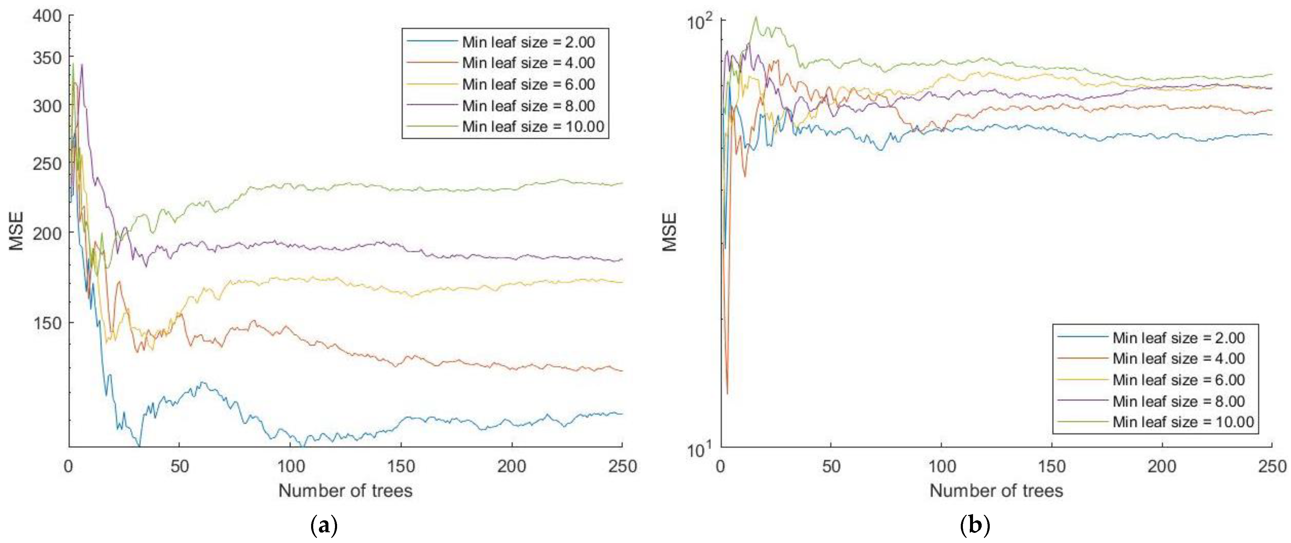
Ensembles of regression trees were realized using random forests and boosting. In case of random forests, the hyperparameters to be optimized were the number of trees and the minimum leaf size. A grid search was used for the optimization. An example of hyperparameter tuning for the estimation of cellulose fiber recovery in the sink product (E_m) is shown in Figure 2a in case the surfactant is oleic acid, and in Figure 2b, in case the surfactant is oleic acid + CaCl₂. In general, more trees usually lead to better estimates; however, note that after 100 trees in Figure 2a and 50 trees in Figure 2b, the MSE mostly stabilizes and there is no point to further increase the number of trees, since this would increase the model complexity. The minimum leaf size determines the smallest number of observations a node is allowed to have. If a child node should be created by splitting with fewer observations than the minimum leaf size, the node is not split. Note that the most accurate models are obtained for the smallest minimum leaf sizes (equal to two in our experiments). However, this leads to deeper trees; so, better performance comes at the cost of increased complexity.

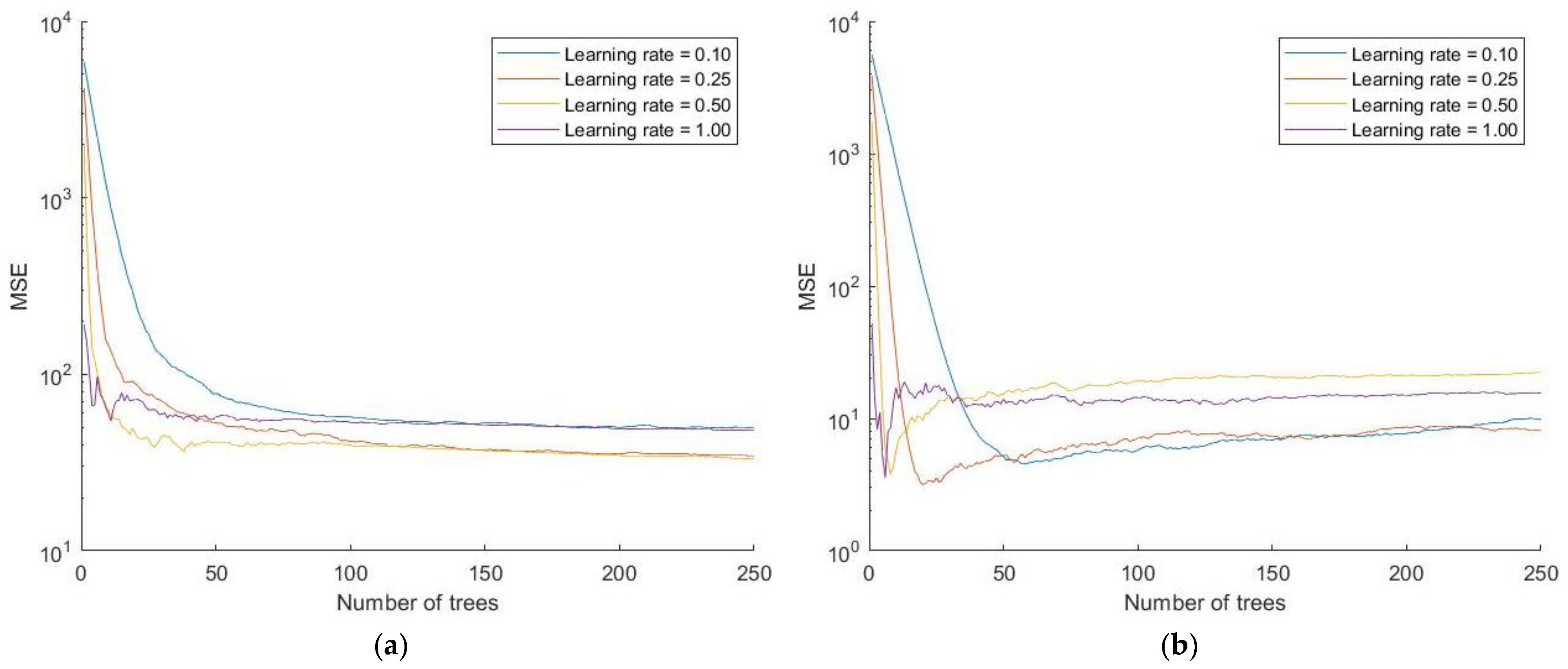
In the case of boosting, the number of trees and the learning rate are optimized using a grid search. An example of hyperparameter tuning for the estimation of cellulose fiber recovery in the sink product (E_m) is shown in Figure 3a, in case the surfactant is oleic acid, and in Figure 3b, in case the surfactant is oleic acid + CaCl₂. As in the case of random forests, the MSE mostly stabilizes for more than 50 trees and there is no point to further increase the number of trees, since this would increase the model complexity. The learning rate is a number between 0 and 1, which multiplies the step magnitude in each gradient step and defines how quickly the prediction error is corrected in the subsequent tree of the model. In other words, shrinkage appears in each gradient step. A learning rate equal to 1 means there is no shrinkage. Small learning rates cause sample predictions to slowly converge towards the observed values and can improve the model’s generalization ability. However, smaller learning rates require larger trees and might become computationally expensive. The learning rate equal to 0.25 is the most optimal in our experiments.

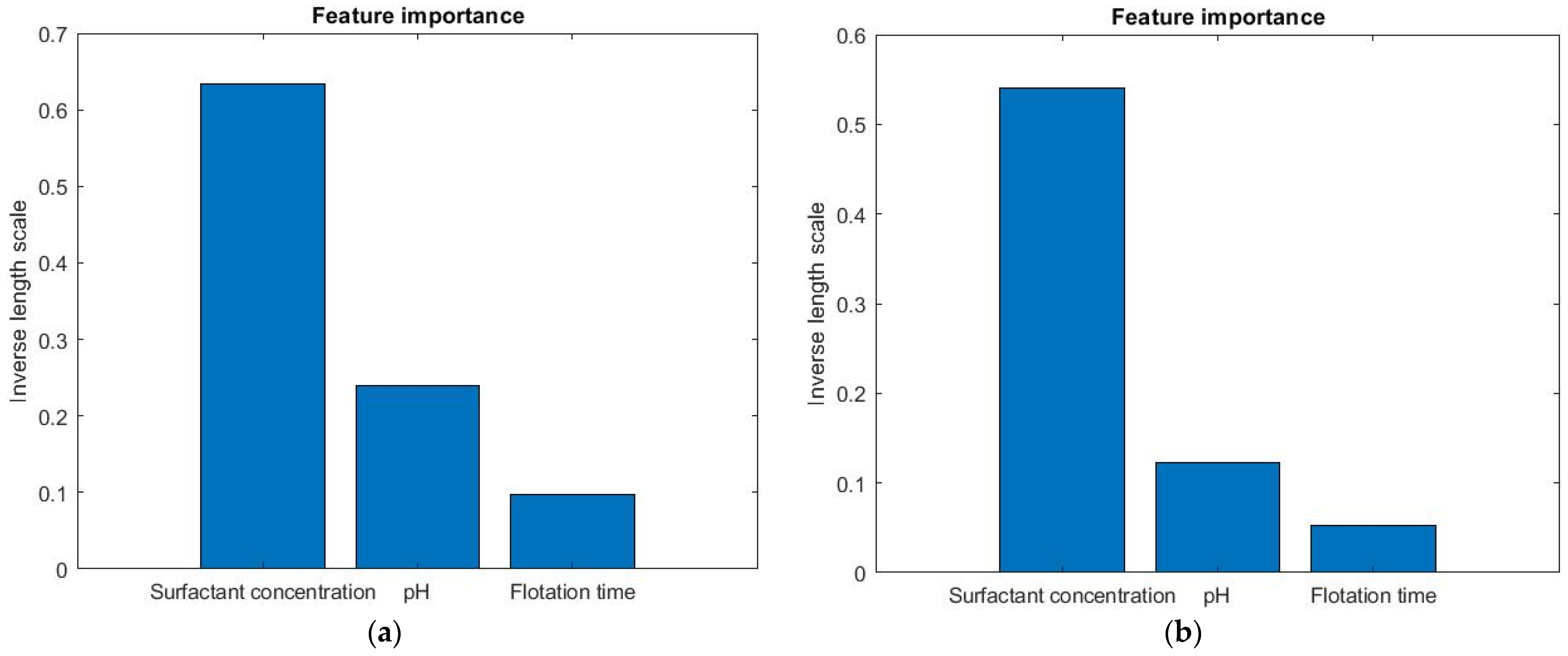
GPR is realized with exponential, squared exponential, Matérn 3/2, Matérn 5/2 and rational quadratic covariance functions. It is further combined with ARD to determine the feature importance, as shown in Figure 4. The length scale is the parameter that estimates the relevance of the input features to predict the model’s response. A small length scale indicates a highly relevant feature and vice versa. The surfactant concentration for both surfactants is the most important feature, whereas the flotation time has the smallest impact on the overall model performance.

Table 3. Estimation of fiber recovery in the sink product (E_m); oleic acid and oleic acid + CaCl₂ were used as surfactants.

Models		Oleic Acid		Oleic Acid + CaCl2
		MSE	R2 [%]	MSE	R2 [%]
SVR	Linear	101.33	63.72	104.24	71.02
	RBF	20.31	93.56	30.97	93.37
Regression trees	Random forests	51.31	88.19	44.47	92.06
	Boosting	21.16	94.05	24.27	93.87
GPR	Exponential	24.06	94.87	27.67	93.34
	Squared exponential	11.85	97.32	19.72	95.43
	Matérn 3/2	14.03	97.66	19.73	95.95
	Matérn 5/2	12.64	97.77	20.21	95.73
	Rational quadratic	12.48	97.66	21.44	95.24

and

Table 4. Estimation of toner recovery in the foam product (E_t); oleic acid and oleic acid + CaCl₂ were used as surfactants.

Models		Oleic Acid		Oleic Acid + CaCl2
		MSE	R2 [%]	MSE	R2 [%]
SVR	Linear	82.20	49.22	56.24	43.91
	RBF	12.52	90.95	19.71	73.96
Regression trees	Random forests	31.80	84.01	29.12	63.96
	Boosting	7.33	93.90	7.95	88.33
GPR	Exponential	24.37	84.50	32.13	64.83
	Squared exponential	45.43	69.07	40.45	55.48
	Matérn 3/2	20.27	86.31	30.87	65.80
	Matérn 5/2	21.62	84.51	38.05	55.83
	Rational quadratic	21.57	84.94	35.98	60.88

present the prediction results of the flotation deinking performance using various machine learning techniques. The fiber recovery in sink product (E_m) and the toner recovery in foam product (E_t) were used to estimate the performance of flotation deinking in Table 3 and Table 4, respectively. Oleic acid and oleic acid with addition of CaCl₂ were used as the surfactants in both cases.

The prediction results for E_m in Table 3 show that GPR with all covariance functions outperforms all other techniques by a large margin using both MSE and R² as performance measures for prediction. The best overall result for R² is obtained using the Matérn 5/2 covariance function when oleic acid was used as the surfactant (R² = 97.77%), whereas the Matérn 3/2 covariance function yields the best performance when CaCl₂ was added to oleic acid (R² = 95.95%). On the other hand, the squared exponential covariance function gives the best estimation for both surfactants when MSE was used as the performance measure. Boosting and SVR with the RBF kernel have comparable performances, which is 2–4% lower than GPR (measured by R²), while the performance of SVR with the linear kernel is significantly worse, due to highly nonlinear dependencies between input data. Based on the presented results, it is shown that GPR using the squared exponential covariance function gave the best performance in the assessment of fiber recovery in the sink product considering MSE as the performance measure. The prediction results for E_t presented in Table 4 are, in general, lower than for E_m. However, boosting outperforms all other machine learning techniques significantly for both performance measures, which is especially evident when oleic acid with the addition of CaCl₂ was used as the surfactant, where the second-best results were 15% lower, measured by R². The dataset is limited (only 100 observations) and it is obviously not enough to capture the complex dependencies between the input features. However, boosting proved to be especially robust to our small-sample problem. The reason might be that boosting, as an ensemble method, can decrease the variance of a single estimate by combining more estimates from different models. Moreover, boosting, unlike random forests, can also reduce the bias by focusing on a weak single model and trying to decrease the prediction error in the next iteration, resulting in a model with higher stability.

4. Conclusions

A comprehensive comparative analysis of a variety of machine learning algorithms for the prediction of flotation deinking performance in the process of paper recycling is given in this paper. A dataset is created for training the models that assumes data samples obtained under a variety of experimental conditions, including different reagents, pH values and flotation residence times. The developed dataset is limited and includes only 100 representative observations, as the aim was to prove that it was feasible to learn reasonable models from “small data” and avoid running expensive, laborious and time-consuming experiments. In this way, it is possible to determine the optimal experimental conditions for the separation of toner particles and cellulose fibers in printed paper recycling using flotation deinking, with only minimal costs and effort.

The obtained results indicate that boosting proved to be especially robust to the small-sample problem under all analyzed conditions. On the other hand, GPR gave the best performance in the estimation of fiber recovery in the sink product, with R² = 97.77%, and also a reasonable performance in the estimation of toner recovery in the foam product, with R² = 86.31%. Another major advantage of GPR is its low complexity in comparison to ensemble models, such as random forests and boosting, which allows an efficient model training and inference.

This study is limited to selected variables that have been reported to have a significant effect on flotation. The scope of the database was limited to the laboratory scale. Machine learning for the optimization of such variables in the real conditions of the flotation process, as proposed in the paper, is only a theoretical approach at this time. Indeed, some machine learning applications still largely remain a relatively new area of research in mineral processing [10], especially in paper flotation.

References

1. Jovanovic, I.; Miljanović, I.; Jovanović, T. Soft computing-based modeling of flotation processes—A review. Miner. Eng. 2015, 84, 34–63. [Google Scholar] [CrossRef]
2. Mohammed, A.S.; Qarani, A.S. Dissolved Air Flotation (DAF): Operational Parameters and Limitations for Wastewaters Treatment with Cost Study. Recycl. Sustain. Dev. 2023, 16, 91–97. [Google Scholar] [CrossRef]
3. Mehari, A. Deinking of Black Toner Ink from Laser Printed Paper by Using Anionic Surfactant. Master’s Thesis, Addis Ababa University, Addis Ababa, Ethiopia, 2017. [Google Scholar]
4. Pauck, W.J.; Venditti, R.; Pocock, J.; Andrew, J. Neural network modelling and prediction of the flotation deinking behaviour of industrial paper recycling processes. Recycl. Nord. Pulp Pap. Res. J. 2014, 29, 521–532. [Google Scholar] [CrossRef]
5. Costa, C.A.; Rubio, J. Deinking flotation: Influence of calcium soap and surface-active substance. Miner. Eng. 2005, 18, 59–64. [Google Scholar] [CrossRef]
6. Pauck, W.J.; Venditti, R.; Pocock, J.; Andrew, J. Using statistical experimental design techniques to determine the most effective variables for the control of the flotation deinking of mixed recycled paper grades. Tappsa J. 2012, 2, 28–41. [Google Scholar]
7. Husovska, V. Investigation of Recycled Paper Deinking Mechanisms. Ph.D. Thesis, Western Michigan University, Kalamazoo, MI, USA, 2013. [Google Scholar]
8. Abraha, M.; Kifle, Z. Deinking of Black Toner Ink from Laser Printed Paper by Using Anionic Surfactant. Chem. Biomol. Eng. 2019, 4, 23–30. [Google Scholar] [CrossRef]
9. Kumar, A.; Dutt, D. A comparative study of conventional chemical deinking and environment-friendly bio-deinking of mixed office wastepaper. Sci. Afr. 2021, 12, e00793. [Google Scholar] [CrossRef]
10. Gomez-Flores, A.; Heyes, G.W.; Ilyas, S.; Kim, H. Prediction of grade and recovery in flotation from physicochemical and operational aspects using machine learning models. Miner. Eng. 2022, 183, 107627. [Google Scholar] [CrossRef]
11. Labidi, J.; Pelach, M.A.; Turon, X.; Mutje, P. Predicting flotation efficiency using neural networks. Intensification 2007, 46, 314–322. [Google Scholar] [CrossRef]
12. Verikas, A.; Malmqvist, K.; Bacauskiene, M. Monitoring the De-Inking Process through Neural Network-Based Colour Image Analysis. Neural Comput. Appl. 2000, 9, 142–151. [Google Scholar] [CrossRef]
13. Laperrière, L.; Wasik, L. Modeling and simulation of pulp and paper quality characteristics using neural networks. Tappi J. 2001, 84, 59. [Google Scholar]
14. Lü, Q.; Liu, S.; Mao, W.; Yu, Y.; Long, X. A numerical simulation-based ANN method to determine the shear strength parameters of rock minerals in nanoscale. Comput. Geotech. 2024, 169, 106175. [Google Scholar] [CrossRef]
15. Nakhaei, F.; Irannajad, M. Application and comparison of RNN, RBFNN and MNLR approaches on prediction of flotation column performance. Int. J. Min. Sci. Technol. 2015, 25, 983–990. [Google Scholar] [CrossRef]
16. Chehreh Chelgania, S.; Shahbazib, B.; Hadavandi, E. Support vector regression modeling of coal flotation based on variable importance measurements by mutual information method. Measurement 2018, 114, 102–108. [Google Scholar] [CrossRef]
17. Szmigiel, A.; Apel, D.B.; Skrzypkowski, K.; Wojtecki, L.; Pu, Y. Advancements in Machine Learning for Optimal Performance in Flotation Processes: A Review. Minerals 2024, 14, 331. [Google Scholar] [CrossRef]
18. Vapnik, V. The Nature of Statistical Learning Theory; Springer: New York, NY, USA, 1995. [Google Scholar] [CrossRef]
19. Vapnik, V.; Golowich, S.; Smola, A. Support vector method for function approximation, regression estimation, and signal processing. In Advances in Neural Information Processing Systems; Mozer, M.C., Jordan, M.I., Petsche, T., Eds.; MIT Press: Cambridge, MA, USA, 1997; Volume 9, pp. 281–287. [Google Scholar]
20. Smola, A.J.; Schölkopf, B. A tutorial on support vector regression. Stat. Comput. 2004, 14, 199–222. [Google Scholar] [CrossRef]
21. Kovačević, M.; Ivanišević, N.; Petronijević, P.; Despotović, V. Construction cost estimation of reinforced and prestressed concrete bridges using machine learning. Građevinar 2021, 73, 1–13. [Google Scholar] [CrossRef]
22. Hastie, T.; Tibshirani, R.; Friedman, J. Boosting and Additive Trees. In The Elements of Statistical Learning; Springer Series in Statistics; Springer: New York, NY, USA, 2009. [Google Scholar] [CrossRef]
23. Cormen, T.H.; Leiserson, C.E.; Rivest, R.L.; Stein, C. Introduction to Algorithms, 3rd ed.; The MIT Press: Cambridge, MA, USA, 2009. [Google Scholar]
24. Despotovic, V.; Skovranek, T.; Schommer, C. Speech Based Estimation of Parkinson’s Disease Using Gaussian Processes and Automatic Relevance Determination. Neurocomputing 2020, 401, 173–181. [Google Scholar] [CrossRef]
25. Rasmussen, C.E.; Williams, C.K.I. Gaussian Processes for Machine Learning; The MIT Press: Cambridge, MA, USA, 2006. [Google Scholar]
26. Lin, D.; Kuang, Y.; Chen, G.; Kuang, Q.; Wang, C.; Zhu, P.; Peng, C.; Fang, Z. Enhancing moisture resistance of starch-coated paper by improving the film forming capability of starch film. Ind. Crops Prod. 2017, 100, 12–18. [Google Scholar] [CrossRef]
27. Dorris, G.M.; Sayegh, N.N. The role of print layer thickness and cohesiveness on deinking of toner printed papers. Tappi J. 1997, 80, 181–191. [Google Scholar]
28. Azevedo, M.A.D.; Drelich, J.; Miller, J.D. The Effect of pH On Pulping and Flotation of Mixed Office Wastepaper. J. Pulp Pap. Sci. 1999, 25, 317–320. [Google Scholar]
29. Dorris, G.; Ben, Y.; Richard, M. Overview of flotation Deinking, Progress in paper recycling. Tappi J. 2011, 20, 3–43. [Google Scholar]
30. Gong, R. New Approaches on Deinking Evaluations. Ph.D. Thesis, Western Michigan University, Kalamazoo, MI, USA, 2013. [Google Scholar]
31. Yilmaz, U.; Tutus, A.; Sönmez, S. Effects of using recycled paper in inkjet printing system on colour difference. Pigment. Resin Technol. 2022, 51, 336–343. [Google Scholar] [CrossRef]
32. Muangnamsuk, R.; Chuetor, S.; Kirdponpattara, S. Development and Optimization of Chemical Deinking of Laser-Printed Paper. Mater. Sci. Forum 2023, 1098, 151–155. [Google Scholar] [CrossRef]
33. Behin, J.; Vahed, S. Effect of alkyl chain in alcohol deinking of recycled fibers by flotation process. Colloids Surf. A Physicochem. Eng. Asp. 2007, 297, 131–141. [Google Scholar] [CrossRef]
34. Jiang, C.; Ma, J. Deinking of waste paper: Flotation. In Encyclopedia of Separation Science; Academic Press: London, UK, 2000; pp. 2537–2544. [Google Scholar]
35. Tsatsis, D.E.; Valta, K.A.; Vlyssides, A.G.; Economides, D.G. Assessment of the impact of toner composition, printing processes and pulping conditions on the deinking of office waste paper. J. Environ. Chem. Eng. 2019, 7, 103258. [Google Scholar] [CrossRef]
36. Ghanbarzadeh, B.; Ataeefard, M.; Etezad, S.M.; Mahdavi, S. Optical and Printing Properties of Deinked Office Waste Printed Paper. Prog. Color Color. Coat. 2024, 17, 75–84. [Google Scholar]
37. Yilmaz, U. Investigation of deinking efficiencies of trigromi laserjet printed papers depending on the number of recycling. Pigment. Resin Technol. 2024, 53, 475–483. [Google Scholar] [CrossRef]
38. Ali, T.; McLellan, F.; Adiwinata, J.; May, M.; Evants, T. Functional and perfomance characteristics of solube silicate in deinking. Part I: Alkaline deinking of newsprint/magazine. J. Pulp Pap. Sci. 1994, 20, J3–J8. [Google Scholar]
39. Liphard, M.; Schereck, B.; Hornfeck, K. Surface chemical aspects of filler flotation in waste paper recycling. Pulp Pap. Can. 1993, 94, 218–222. [Google Scholar]
40. Luo, Q.; Deng, Y.; Zhu, J.; Shin, W.T. Foam control using a foaming agent spray: A novel concept for flotation deinking of waste paper. Ind. Eng. Chem. Res. 2003, 15, 3578–3583. [Google Scholar] [CrossRef]
41. Pathak, P.; Bhardwaj, N.K.; Singh, A.K. Optimization of Chemical and Enzymatic Deinking of Photocopier Waste Paper. BioResources 2011, 6, 447–463. [Google Scholar] [CrossRef]
42. Chandranupap, P.; Chandranupap, P. Enzymatic Deinking of Xerographic Waste Paper with Non-ionic Surfactant. Appl. Sci. Eng. Prog. 2020, 13, 136–145. [Google Scholar] [CrossRef]
43. Yilmaz, U.; Tutuş, A.; Sönmez, S. Fiber Classification, Physical and Optical Properties of Recycled Paper. Cellul. Chem. Technol. 2021, 55, 689–696. [Google Scholar] [CrossRef]
44. Despotović, V.; Trumić, M.S.; Trumić, M.Ž. Modeling and prediction of flotation performance using support vector regression. Recycl. Sustain. Dev. 2017, 10, 31–36. [Google Scholar] [CrossRef]
45. Khadka, K.; Chandrasekaran, J.; Lei, Y.; Kacker, R.N.; Kuhn, D.R. A Combinatorial Approach to Hyperparameter Optimization. In Proceedings of the 2024 IEEE/ACM 3rd International Conference on AI Engineering—Software Engineering for AI (CAIN), Lisbon, Portugal, 14–15 April 2024; pp. 140–149. [Google Scholar]
46. Chang, C.C.; Lin, C.J. LIBSVM: A Library for Support Vector Machines. ACM Trans. Intell. Syst. Technol. 2011, 2, 1–27. [Google Scholar] [CrossRef]
Figure 1. Optimization of the hyperparameters γ and C in SVR with the RBF kernel for estimating cellulose fiber recovery in the sink product (Em) when the surfactant is (a) oleic acid and (b) oleic acid + CaCl2.
Applsci 14 08990 g001
Figure 2. Optimization of the hyperparameters minimum leaf size and number of trees in random forests for estimating cellulose fiber recovery in the sink product (Em) when the surfactant is (a) oleic acid and (b) oleic acid + CaCl2.
Applsci 14 08990 g002
Figure 3. Optimization of the hyperparameters learning rate and number of trees in boosting for estimating cellulose fiber recovery in the sink product (Em) when the surfactant is (a) oleic acid and (b) oleic acid + CaCl2.
Applsci 14 08990 g003
Figure 4. Feature selection using ARD in GPR for estimating cellulose fiber recovery in the sink product (Em) when the surfactant is (a) oleic acid and (b) oleic acid + CaCl2.
Applsci 14 08990 g004