A Study on the Coarse-to-Fine Error Decomposition and Compensation Method of Free-Form Surface Machining

Abstract

To improve the machining accuracy of free-form surface parts, a coarse-to-fine free-form surface machining error decomposition and compensation method is proposed in this paper. First, the machining error was coarsely decomposed using variational mode decomposition (VMD), and the correlation coefficients between the intrinsic mode function (IMF) and the machining error were obtained to filter out the IMF components that were larger than the thresholding value of the correlation coefficients, which was the coarse systematic error. Second, the coarse systematic errors were finely decomposed using empirical mode decomposition (EMD), which still filters out the IMF components that are larger than the thresholding value of the set correlation coefficient based on the correlation coefficient. Then, the wavelet thresholding method was utilized to finely decompose all the IMF components whose correlation coefficients in the first two decomposition processes were smaller than the threshold value of the correlation coefficient set. The decomposed residual systematic errors were reconstructed with the IMF components screened in the EMD fine decomposition, which gave the fine systematic error. Finally, the machining surface was reconstructed according to the fine systematic error, and its corresponding toolpath was generated to compensate for the machining error without moving the part. The simulation and analysis results of the design show that the method has a more ideal processing error decomposition ability and can decompose the systematic error contained in the processing error in a more complete way. The results of actual machining experiments show that, after using the method proposed in this paper to compensate for the machining error, the maximum absolute machining error decreased from 0.0580 mm to 0.0159 mm, which was a 72.5% reduction, and the average absolute machining error decreased from 0.0472 mm to 0.0059 mm, which was an 87.5% reduction. It was shown that the method was effective and feasible for free-form surface part machining error compensation.

1. Introduction

1.1. Problem Statement of Motivation and Methodology

Currently, with the continuous increase in expected aesthetic requirements and the simultaneous development of manufacturing technology, there are an increasing number of parts containing free-form surfaces in daily life [1]. To meet the needs of various industries for CNC machining accuracy and efficiency, CNC machine tools have been constantly and rapidly developed in the direction of high precision and intelligence. Due to the more complex geometric structure of free-form surface parts, such parts are generally processed by CNC machine tools. There are many factors that lead to machining errors, mainly geometric, force and thermal errors [2]. Improving the machining accuracy of CNC machine tools has more important research significance, and error compensation is an effective and economic means to improve the machining accuracy of CNC machine tools [3].

In this paper, a coarse-to-fine free-form surface machining error decomposition and compensation method was proposed which was based on the principles of decomposing the machining error from coarse to fine by variational mode decomposition (VMD)-EMD combined with the wavelet thresholding method and compensating for the decomposed systematic error. The geometric model of the free-form surface part was imported into Mastercam 2021 software to generate the corresponding NC code, which was then imported into the CNC for roughing and semifinishing. First, on-machine measurements were performed after semifinish machining was completed to obtain measurement point data on the surface of the free-form surface part, and then the machining error of each measurement point was calculated [4]. Second, the machining error was decomposed into the systematic error and random error using VMD-EMD combined with the wavelet thresholding method. Finally, the surface was reconstructed according to the decomposed systematic error to obtain the machined surface after compensating for the systematic error, generating the corresponding NC code and completing the compensated machining. This method can reduce the machining error of the free-form surface part to a greater extent and does not need to transfer or restrain the part to realize machining error compensation, which has more important research significance.

1.2. Literature Review

Liu et al. [5] proposed a generalized practical inverse kinematics model that compensates for geometrical errors in five-axis machine tools which provides explicit solutions for compensated motion commands and can be directly applied to five-axis machine tools of any configuration, especially those with nonorthogonal rotational axes. However, this method requires several iterations of computation for ultraprecision machining to achieve predetermined accuracy. Li et al. [6] proposed an automatic approximation modeling algorithm based on the combination of moving least squares and Chebyshev polynomials for applying geometric error parameters, but the compensation effect of this method decreases when the continuity and consistency of the geometric error curve are poor. Msaddek et al. [7] proposed a spline interpolation machining error compensation method based on B-splines and C-splines by inserting nodes into the tool trajectory to minimize machining error, but this method affects the surface machining quality of parts with complex shapes. Fu et al. [8] proposed a method for automatic modeling of position-related geometric error components based on a statistical F test and a method for compensating for geometric errors by restricting the ideal tool position, which ensures the workpiece texture during machining on five-axis machine tools and better compensates for the machining error. Wu et al. [9] proposed an error compensation algorithm based on the chi-square transformation to derive a geometric error model and then reconstructed the CNC machining code according to the geometric error model. However, the method only compensates for the geometric error and does not consider the effect of other errors on the machining accuracy. Chen et al. [10] used empirical mode decomposition (EMD) to decompose machining errors into systematic and random errors and compensated for systematic errors by modifying the NC code. This method can improve the machining accuracy of the workpiece, but some shortcomings of EMD itself lead to a poor compensation effect. Lin et al. [11] proposed a geometric error identification and compensation method for measuring the volume diagonal error of CNC machine tools. This method deduces the error identification equations of geometric errors by several factors, then uses a regularization method to identify geometric error parameters, and, finally, compensates the geometric errors identified. Zhang et al. [12] proposed an optimization model of a machining allowance for complex parts based on coordinate measuring machine (CMM) inspection by first establishing a mathematical model of constraint alignment and then proposing a symmetric block solving strategy to solve the optimization model, which can effectively reduce the machining error. Li et al. [13] proposed a combination algorithm based on the bat algorithm of a back-propagation neural network for solving the thermal error modeling problem. The algorithm establishes a high prediction accuracy of the thermal positioning error model, which can better compensate for the thermal error, but the compensation effect was only verified on the three-axis experimental bench, and the actual cutting state of the thermal error model still needs further research. Reddy et al. [14] used a feed-forward neural network to establish a thermal error compensation model and then used regression analysis technology to simplify the model to achieve real-time compensation of thermal errors in precision machine tools. However, their network failed to eliminate the effects of geometric and process errors; for ordinary machine tools, the error compensation effect was not very obvious. Wei et al. [15] proposed a method to compensate the geometric error by using an improved genetic algorithm, established the actual and theoretical motion model of the machine tool through the homogeneous transformation matrix, reduced the initial population range and changed the chromosome selection value in the convergence range to improve the genetic algorithm, so as to obtain the error compensation value. Zha et al. [16] proposed an “evolutionary” method to improve the machining accuracy of the surface, the essence of which is to compensate the machining error of the first part by measuring the profile error.

2. The Coarse-to-Fine Free-Form Surface Machining Error Decomposition and Compensation Process

Theoretically, a machining error consists of the systematic error and random error, and, in general, the random error is smaller than the systematic error [17]. The random error is highly random and uncertain and cannot be measured precisely, making compensation more difficult. The systematic error is characterized by repeatability, measurability and unidirectionality, making it less difficult to compensate for such errors.

This paper mainly utilizes VMD-EMD combined with the wavelet thresholding method to decompose the systematic error contained within the machining error and then compensates for the systematic error. After the completion of roughing and semifinishing, the machining error corresponding to each measurement point was obtained via on-machine measurement, and the machining error was decomposed via VMD-EMD combined with the wavelet thresholding method. In the process of decomposition, correlation coefficients were introduced to quickly and accurately screen out the intrinsic modal function (IMF) components of the machining error that contain the systematic error. After the systematic error was decomposed from the processing error using the method proposed in this paper, it was added to the original coordinates of the corresponding measurement point along the opposite direction of the outer normal vector of the measurement point to obtain the compensated measurement point coordinates. Finally, surface reconstruction was carried out according to the coordinates of the compensated measurement points [18] to obtain the free-form surface after systematic error compensation, and 3D modeling was completed according to this free-form surface. To ensure that the conditions remain unchanged in subsequent machining, the compensating machining parameters were set to be the same as the semifinishing machining parameters to obtain the compensating machining toolpath NC code, which was the finishing toolpath [19].

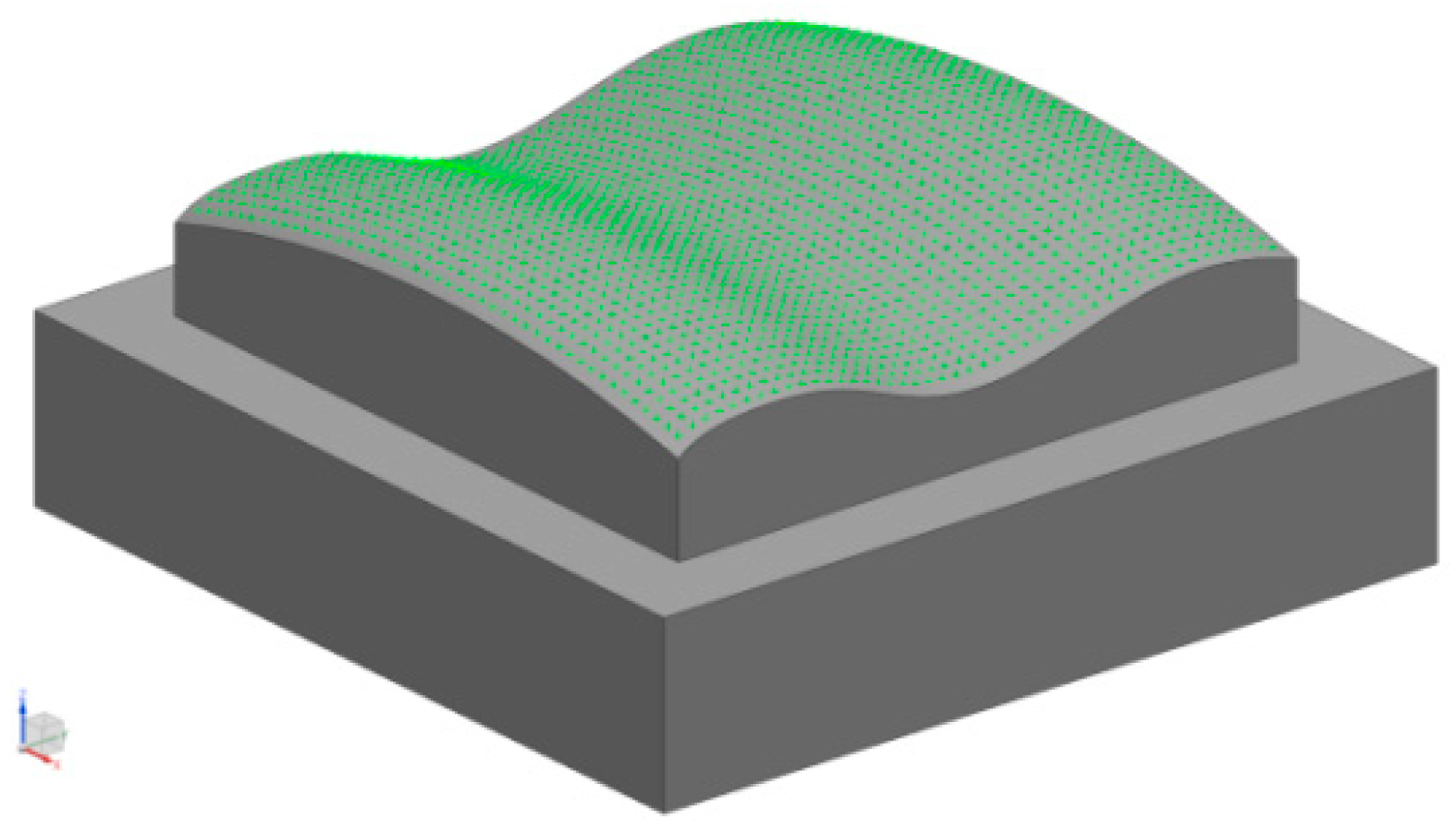
2.1. Calculation of the Machining Error for the Free-Form Surface Part

During CNC machining of a free-form surface, numerous factors, such as the machining accuracy of the machine itself, tool wear and thermal deformation, can cause machining errors. The machining error of the free-form surface part was obtained by on-machine measurement, as shown in Equation (1) [20]:

$$\delta =\sqrt{{\left(x_m-x\right)}^2+{\left(y_m-y\right)}^2+{\left(z_m-z\right)}^2}$$

(1)

where $\left(x_m,y_m,z_m\right)$ is the actual coordinate data measured at a measurement point, and $\left(x,y,z\right)$ is the coordinate of the nearest point on the ideal surface to the actual measurement point. Therefore, the machining error at each measurement point was the shortest distance from the actual coordinates of that measurement point to the ideal surface.

2.2. Correlation Coefficient Principle

The correlation coefficient r reflects the strength of the linear correlation between two variables, and a larger absolute value of r indicates a stronger degree of linear correlation between the two variables [21]. Assuming that there are two pooled samples of length n, $\left\{x_1,x_2,x_3,\cdots ,x_n\right\}$ and $\left\{y_1,y_2,y_3,\cdots ,y_n\right\}$, the correlation coefficient r is calculated as shown in Equation (2) [22]:

$$r={\displaystyle \frac{{\displaystyle \sum _{i=1}^n(x_i-\overline{x})(y_i-\overline{y})}}{\sqrt{{\displaystyle \sum _{i=1}^n{(x_i-\overline{x})}^2}}\sqrt{{\displaystyle \sum _{i=1}^n{(y_i-\overline{y})}^2}}}}$$

(2)

where $\overline{x}$ and $\overline{y}$ are the means of the two pooled samples, and r is $[-1,1]$.

When the absolute value of the correlation coefficient is less than 0.3, there is a weak correlation between the corresponding IMF component and the original processing error [23]. Therefore, the correlation coefficient thresholding was set to 0.3 in this paper.

2.3. Principle of Machining Error Decomposition from Coarse to Fine

2.3.1. Principle of the VMD Algorithm

Dragomirestkiy et al. [24] proposed the VMD algorithm, which is essentially the construction and solution of variational models. The algorithm is based on the mathematical theories of Wiener filtering, Hilbert transform and frequency mixing and aims to decompose a real-valued analyzed signal into K IMFs by nonrecursive filtering, which compensates for the shortcomings of cyclic recursive filters. It also has good results in processing nonlinear and nonsmooth signals. The algorithm flow of VMD is as follows [25].

1.

Construction of constrained variational models

It is assumed that the original signal is decomposed into K IMF components, each of which is a narrow-bandwidth signal distributed near the center frequency. The constrained variational model is constructed depending on the sparsity of the narrow-bandwidth components in the frequency domain, and the original signal is equal to the sum of all the IMF components. This constrained variational model can be expressed by

$$\left\{\begin{array}{c}\underset{\left\{u_k\right\},\left\{{\omega }_k\right\}}{\min }\left\{{\displaystyle \sum _{k=1}^K{‖{\partial }_t\left[\left(\delta \left(t\right)+\frac{j}{\mathsf{\pi }t}\right)\ast u_k\left(t\right)\right]e^{-j\omega kt}‖}_2^2}\right\}\\ s.t.{\displaystyle \sum _{k=1}^K{u}_k}=x\end{array}\right.$$

(3)

where x is the original signal, $u_k$ corresponds to the K IMF components, ${\partial }_t(·)$ is the partial derivative with respect to time t, $\delta (t)$ is the Dirac distribution with respect to time t and ${\omega }_k$ is the center frequency of $u_k(t)$.

2.

Solution of the constrained variational model

First, the constrained variational model is reconstructed by introducing a quadratic penalty factor and a Lagrange multiplier term. The quadratic penalty is a classic way to encourage reconstruction fidelity, typically in the presence of additive i.i.d. Gaussian noise. The weight of the penalty term is derived from such a Bayesian prior to be inversely proportional to the noise level in the data. On the other hand, Lagrangian multipliers are a common way of enforcing constraints strictly. The combination of the two terms thus benefits both from the nice convergence properties of the quadratic penalty at finite weight and the strict enforcement of the constraint by the Lagrangian multiplier. The quadratic penalty term allows the algorithm to converge quickly and improve the model reconstruction accuracy, and the Lagrange multiplier term transforms the constrained variational model into an unconstrained variational model. The reconstructed unconstrained variational model can be expressed by

$$\begin{array}{ll}L\left(\left\{u_k\right\},\left\{{\omega }_k\right\},\lambda \right)=& \alpha {{\displaystyle \sum _{k=1}^K‖{\partial }_t\left[\left(\delta (t)+\frac{j}{\mathsf{\pi }t}\right)\ast u_k\left(t\right)\right]e^{-j\omega kt}‖}}_2^2+\\ & {‖x\left(t\right)-{\displaystyle \sum _{k=1}^K{u}_k\left(t\right)}‖}_2^2+〈\lambda \left(t\right),x\left(t\right)-{\displaystyle \sum _{k=1}^K{u}_k(t)}〉\end{array}$$

(4)

where $L(·)$ is the Lagrange function, $\alpha$ is the quadratic penalty factor and $\lambda (t)$ is the Lagrange multiplier term.

Second, the optimal solution of Equation (4) is searched by an iterative method in the frequency domain, and each IMF component and its corresponding center frequency are updated iteratively according to the alternating direction method of multipliers (ADMM), where the IMF component update equation can be expressed by

$$u_k^{(n+1)}(\omega )={\displaystyle \frac{x(\omega )-{\displaystyle \sum _{k=1}^K{u}_k^{(n+1)}(\omega )+{\displaystyle \sum _{k+1}^K{u}_{k+1}^n(\omega )}}}{1+2\alpha {(\omega -{\omega }_k^n)}^2}}$$

(5)

where $x(\omega )$ is the Fourier transform of $x(t)$, $u_k^{(n)}(\omega )$ is the nth iteration of $u_k(t)$ in the Fourier time domain, $\left\{{\omega }_k^{(n)}\right\}$ is the nth iteration of ${\omega }_k$ and $\omega$ is the frequency parameter. The equation for updating the center frequency of each IMF component can be expressed by

$${\omega }_k^{(n+1)}={\displaystyle \frac{{\displaystyle {\int }_0^{\infty }\omega {\left|u_k^{(n+1)}(\omega )\right|}^{2}d\omega }}{{\displaystyle {\int }_0^{\infty }{\left|u_k^{(n+1)}(\omega )\right|}^{2}d\omega }}}$$

(6)

Assume that the number of iterations in the whole solution process is n. The iterative termination condition of the above update process can be expressed by

$${\displaystyle \frac{{\displaystyle \sum _{k=1}^K{‖u_k^{(n+1)}(\omega )-u_k^n(\omega )‖}_2^2}}{{‖u_k^n(\omega )‖}_2^2}}<\epsilon$$

(7)

where $\epsilon$ is the convergence parameter, generally taken as $1\times {10}^{-7}$.

Finally, the Lagrange multiplier term is updated based on each IMF component obtained by iterative updating and its corresponding center frequency. Its update equation can be expressed by

$${\lambda }^{\left(n+1\right)}\left(\omega \right)={\lambda }^{\left(n\right)}\left(\omega \right)+\tau \left(x\left(\omega \right)-{\displaystyle \sum _{k=1}^K{u}_k^{\left(n+1\right)}}\right)$$

(8)

where ${\lambda }^{(n)}(\omega )$ is the nth iteration value of $\lambda (t)$ in the Fourier time domain, and $\tau$ is the step size of the Lagrange multiplier term.

2.3.2. Principle of the EMD Algorithm

The EMD algorithm is a new adaptive signal time–frequency processing method proposed by Huang in 1998 [26]. The algorithm can decompose an arbitrary signal into a number of IMF components, which is not only applicable to linear and smooth signals but also has good results in processing nonlinear and nonsmooth signals. Its essence is the decomposition of complex signals from high and low frequencies into individual intrinsic modal function components according to the time scale [27]. EMD decomposes the original signal into several IMFs, and each IMF has the following two characteristics:

(1)

Within the entire signal, the number of extremum and zero crossing points must be the same, and the number of both must not differ by more than one at most;

(2)

At any point within the signal, the upper envelope consisting of local maximum values and the lower envelope consisting of local minimum values both have an average value of 0, which is the local mean value.

The specific decomposition steps of the EMD algorithm are as follows:

(1)

Assuming that $x(t)$ is the average of the upper and lower envelopes of the original signal $m_1(t)$ and that $h_1(t)$ is the difference between $x(t)$ and $m_1(t)$, it can be expressed by

$$h_1(t)=x(t)-m_1(t)$$

(9)

Determine whether $h_1(t)$ in Equation (9) satisfies the characteristics of the IMF component. If $h_1(t)$ satisfies the condition, then $h_1(t)$ is the first IMF component of $x(t)$. The reason is that, in the actual decomposition process, overshooting and undershooting occur when fitting the envelope, and, in general, $h_1(t)$ does not satisfy the conditions of the IMFs.

(2)

Treating $h_1(t)$ as the signal to be decomposed and repeating step (1), it can be expressed by

$$h_{11}(t)=h_1(t)-m_{11}(t)$$

(10)

After performing k decompositions, the following can be obtained:

$$h_{1k}(t)=h_{1(k-1)}(t)-m_{1k}(t)$$

(11)

Decomposition ends when the final obtained $h_{1k}(t)$ satisfies the two conditions of the IMF and $h_{1k}(t)$ is the first IMF component of the original signal $x(t)$, which is IMF1 and is denoted as $c_1(t)$:

$$c_1(t)=h_{1k}(t)$$

(12)

Since the upper and lower envelopes mean that $m_{1k}(t)$ cannot be zero during the actual decomposition process, a stopping criterion must be determined to ensure that the decomposition process ends. For this reason, Huang et al. proposed a stopping criterion for the decomposition as follows:

$$SD={\displaystyle \frac{{\displaystyle \sum _0^T{\left|h_{1(k-1)}(t)-h_{1k}(t)\right|}^2}}{{\displaystyle \sum _0^T{\left|h_{1(k-1)}(t)\right|}^2}}}$$

(13)

A suitable thresholding is set before the decomposition is performed, and the decomposition is stopped immediately when SD is smaller than the set thresholding, typically $SD\in \left[0.2,0.3\right]$.

(3)

Separate $c_1(t)$ from $x(t)$ in the original signal to obtain a new data sequence $r_1(t)$:

$$r_1(t)=x(t)-c_1(t)$$

(14)

Using $r_1(t)$ to replace $x(t)$ as the new original signal and repeating the above decomposition process yield the second component, IMF2, that qualifies as an IMF, which is $c_2(t)$. The cycle is repeated n times to obtain n components eligible for the IMFs as follows:

$$\left.\begin{array}{c}{r}_2(t)=r_1(t)-c_2(t)\\ ⋮\\ r_n(t)=r_{n-1(t)}-c_n(t)\end{array}\right\}$$

(15)

(4)

After decomposition, the original signal $x(t)$ can be expressed as

$$x(t)={\displaystyle \sum _i^n{c}_i(t)+r_n(t)}$$

(16)

2.3.3. Principle of the Wavelet Thresholding Method

Currently, the wavelet transform, which has multiscale and decorrelation properties, is one of the most common time–frequency analysis methods. In the wavelet transform, the selection of the basis function, thresholding function, thresholding rule and number of decomposition layers is highly important. The wavelet basis function selected in this paper is the Daubechies wavelet, abbreviated as db N, where N is the order of the wavelet, which is commonly used to decompose and reconstruct signals with good results. In general, the wavelet thresholding decomposition process can be divided into three steps: wavelet decomposition, thresholding quantization of the high-frequency coefficients of wavelet decomposition and wavelet reconstruction [28].

The commonly used thresholding quantization rules are generally divided into hard and soft thresholding, and the hard thresholding function tends to cause oscillations in the reconstructed signal. Therefore, in this paper, a soft thresholding function is used, which can be expressed by

$${\sigma }_{\lambda }^S=\left\{\begin{array}{cc}\hfill \left[\mathrm{sgn}(\omega )\right](\left|\omega \right|-\lambda )\hfill & ,\left|\omega \right|\ge \lambda \hfill \\ \hfill 0\hfill & ,\left|\omega \right|<\lambda \hfill \end{array}\right.$$

(17)

where $\omega$ is the wavelet coefficient, and $\lambda$ is the thresholding value.

The determination of the thresholding $\lambda$ is an important step in the decomposition of processing errors by the wavelet thresholding method which has a great influence on the decomposition effect. When the thresholding is too small, the decomposition may be incomplete, and interference information may remain; when the thresholding is too large, useful information may be lost. Currently, fixed thresholding, which is based on the Gaussian noise model and derived from the decision theory of independent normal variables, is widely used [29]. This paper chooses to use a fixed thresholding, which can be expressed by

$$\lambda =\sigma \sqrt{2\log n}$$

(18)

where n is the length of the wavelet coefficients, and $\sigma$ is the signal standard deviation.

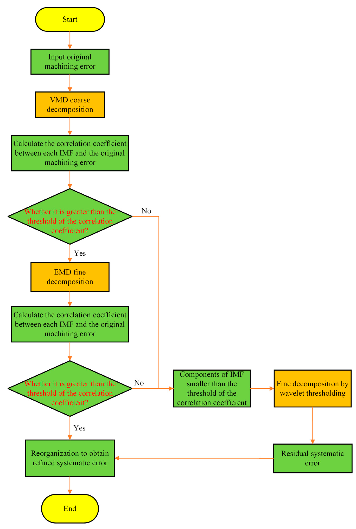
2.3.4. Principle of the Coarse-to-Fine Machining Error Decomposition Method

To accurately decompose the free-form surface machining error, a coarse-to-fine machining error decomposition method is proposed in this paper. The goal of this method is to combine the VMD algorithm, EMD algorithm and wavelet thresholding method, sort the algorithms by considering their characteristics and decompose the processing errors according to the order of the algorithms. The specific steps of its decomposition are as follows:

(1)

Let the original machining error be $x=\left\{x_1,x_2,x_3,\cdots ,x_n\right\}$, and use VMD to coarsely decompose the machining error to obtain K components of IMFs of length n, which can be expressed by

$$x={\displaystyle \sum _{k=1}^K\mathrm{IMF}}k$$

(19)

The correlation coefficients between each of the IMF components and the original machining error are calculated separately to obtain a series of correlation coefficients $r_i$, which can be expressed by

$$r_i={\displaystyle \frac{{\displaystyle \sum _{i=1}^n(x_i-\overline{x})({\mathrm{IMF}}_i-\overline{\mathrm{IMF}})}}{\sqrt{{\displaystyle \sum _{i=1}^n{({\mathrm{IMF}}_i-\overline{\mathrm{IMF}})}^2}}\sqrt{{\displaystyle \sum _{i=1}^n{(x_i-\overline{x})}^2}}}}$$

(20)

The IMF components with absolute correlation coefficients greater than the thresholding set for the correlation coefficients are filtered out and reconstructed to obtain the crude systematic error X₁ after VMD.

(2)

EMD is utilized to perform a fine decomposition of the coarse systematic error X₁ after VMD into M IMF components and a trend term, which can be expressed by

$$X_1={\displaystyle \sum _{m=1}^M\mathrm{IMF}}m+\mathrm{res}$$

(21)

The correlation coefficient between each IMF component obtained from the refined decomposition and the original processing error is calculated. Based on the correlation coefficients, the IMF components that are larger than the thresholding of the set correlation coefficient are filtered out and reconstructed to obtain the systematic error X₂.

(3)

The IMF components with correlation coefficients of less than 0.3 in the VMD coarse decomposition and EMD fine decomposition processes may also contain a small systematic error. To ensure that the decomposed systematic error is as complete and accurate as possible, the weakly correlated IMF components with correlation coefficients of less than 0.3 in the first two decomposition processes are decomposed using the wavelet thresholding method. The random errors are removed, and the systematic errors are retained.

The IMF components’ correlation coefficients between the two processes, VMD coarse decomposition and EMD fine decomposition, and the original machining error are less than the thresholding value of the correlation coefficient set. They are reconstructed and decomposed using the wavelet thresholding method to obtain the systematic error X₃ contained therein.

(4)

The systematic error X₂ decomposed by EMD is reconstructed with the systematic error X₃ decomposed by the wavelet thresholding method to obtain the refined systematic error X₄, which can be expressed by

$$X_4=X_2+X_3$$

(22)

The machining error decomposition process from coarse to fine is shown in Figure 1.

3. Simulation Experiment of Machining Error Decomposition from Coarse to Fine

To verify the feasibility and effectiveness of the coarse-to-fine free-form surface machining error decomposition and compensation method, a simulation experiment involving free-form surface part machining error decomposition was designed for this paper. The model of the free-form surface workpiece and the arrangement of its surface measurement points are shown in Figure 2. The 45 measurement points were generated uniformly along the u and v directions of the free-form surface workpiece, respectively, for a total of 2025 measurement points.

By iteratively adding the simulated machining error to each measurement point, the machining error generated during the actual machining process was simulated. The simulated systematic error is generated by Equation (23), and its value and distribution are shown in Figure 3.

$$x(t)=0.04\times [\sin (1.6\mathsf{\pi }t)+\cos (0.05\mathsf{\pi }t)+4e^{-3t}]$$

(23)

where $t\in \left(1,21.24\right)$, and the step size is 0.01.

The simulated random error was 2025 random numbers generated from a normal distribution $\mathrm{N}(0,0.005)$. The values and distributions are shown in Figure 4.

The simulation machine error was the sum of the simulation systematic error and the simulation random error. Its value and distribution are shown in Figure 5.

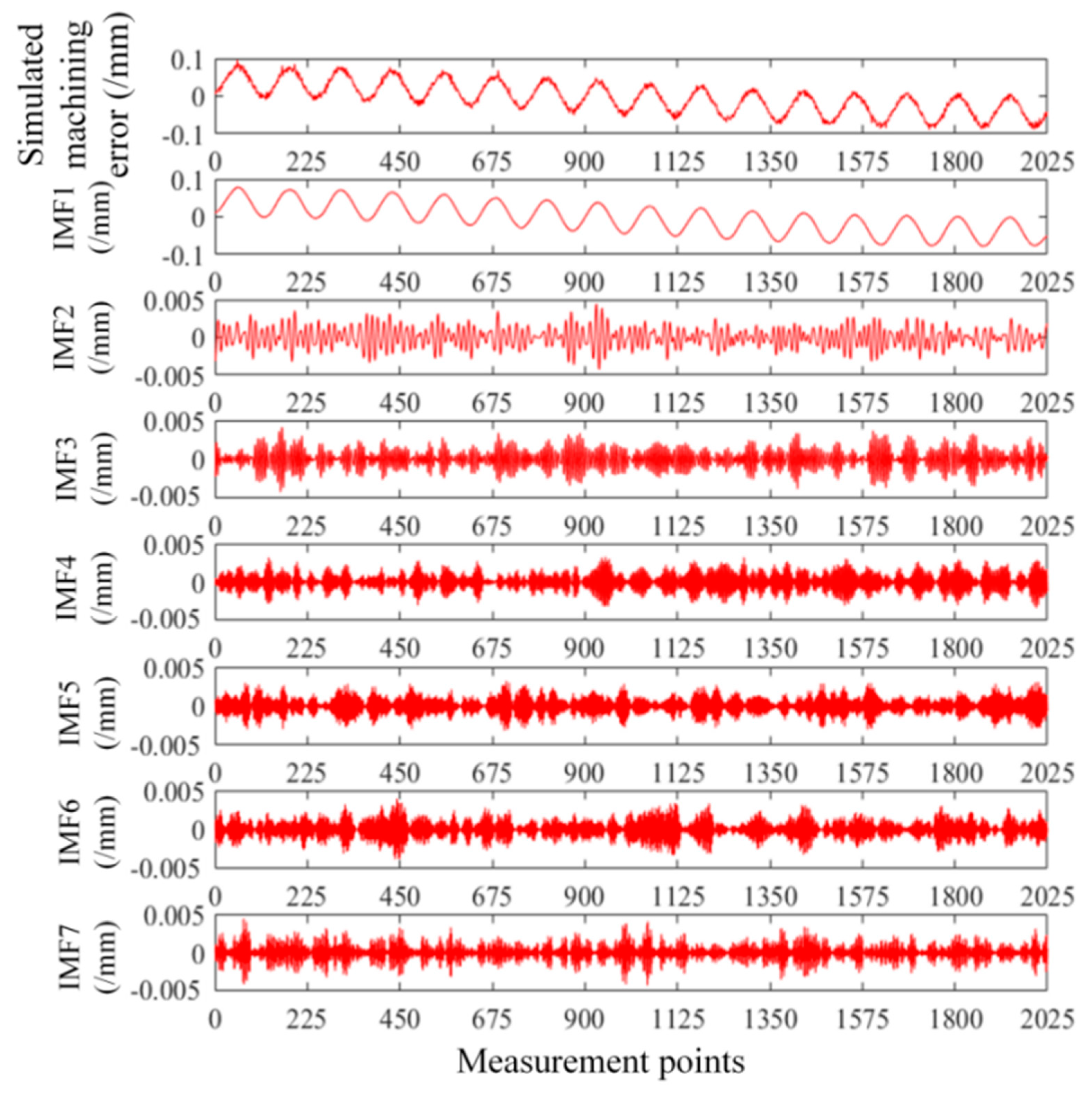
3.1. VMD Algorithm Coarse Decomposition of the Simulation Machining Error

When using the VMD algorithm to decompose machining errors, the number of decomposition layers K has a direct impact on the decomposition accuracy. For this paper, the instantaneous frequency averaging method was used to determine the number of decomposition layers in the VMD [30], and K was analyzed and determined to be 7. Coarse decomposition of the simulated machining error using the VMD algorithm yielded the seven IMF components, and the decomposition results are shown in Figure 6.

The correlation coefficients between each IMF component and the simulated machining error are calculated, as shown in

Table 1. Correlation coefficients between each IMF component and the simulated machining error.

IMF Component	IMF1	IMF2	IMF3	IMF4	IMF5	IMF6	IMF7
correlation coefficient	0.9931	0.1604	0.0743	0.0606	0.0546	0.0534	0.0537

.

Table 1 shows that component IMF1 not only meets the screening conditions but also has a strong correlation with the simulation processing error, meaning that the IMF1 component must contain most of the systematic error. Therefore, the IMF1 component was used as the coarse systematic error X₁ obtained after the coarse decomposition of the simulated machining error using the VMD algorithm.

3.2. EMD Algorithm Fine Decomposition of the Simulation Machining Error

The EMD algorithm is self-adaptive and does not require a priori determination of the number of its decomposition layers. The EMD algorithm was directly used to decompose the coarse systematic error X₁ to obtain three IMF components, and the decomposition results are shown in Figure 7, where IMF3 is the trend term.

The correlation coefficients between each IMF component in Figure 7 and the simulation machining error were calculated separately, as shown in

Table 2. Correlation coefficients corresponding to each IMF component.

IMF Component	IMF1	IMF2	IMF3
correlation coefficient	0.7134	0.0342	0.7125

, and the IMF components that contained systematic errors were filtered out according to correlation coefficient thresholding. As shown in Table 2, the IMF1 and IMF3 components met the screening conditions, indicating that they contained systematic errors. The IMF1 and IMF3 components were reorganized to obtain the systematic error X₂.

3.3. Residual Systematic Error Decomposition by the Wavelet Thresholding Method

During the decomposition of the simulation processing error using the VMD algorithm, the components IMF2, IMF3, IMF4, IMF5, IMF6 and IMF7 did not meet the filtering conditions and were weakly correlated IMF components. During the decomposition of the coarse systematic error X₁ using the EMD algorithm, component IMF2 did not meet the filtering conditions and was a weakly correlated IMF component. Since the weakly correlated IMF components of the two decomposition processes may also contain a small systematic error, to ensure the accuracy of the decomposition results, they were reorganized and decomposed using the wavelet thresholding method to obtain the systematic error X₃.

The systematic error X₃ decomposed by the wavelet thresholding method and the systematic error X₂ decomposed by the EMD algorithm were reorganized to obtain the fine systematic error X₄, which was the part of the systematic error decomposed from coarse to fine from the simulated machining error, and its value and distribution are shown in Figure 8.

3.4. Simulation Results Analysis

By comparing Figure 8 with Figure 3, it can be seen that the fine systematic error X₄ obtained after decomposing the simulated machining error from coarse to fine was very close to the simulated systematic error in terms of value and distribution, indicating that the fine systematic error X₄ decomposed from the simulated machining error by this method was more complete and had a smaller difference from the simulated systematic error. To reflect the decomposition ability of the method more intuitively, the error between the simulated systematic error and the fine systematic error X₄ and the error between the two were used as measures for evaluating its decomposition ability, as shown in Figure 9.

As shown in Figure 9, the mean absolute error between the simulated systematic error and the fine systematic error X₄ was 0.0008 mm, the maximum absolute error was 0.0039 mm and the minimum absolute error was 0 mm. The correlation coefficient between the simulation systematic error and the fine systematic error X₄ was 0.9998. It can be seen that the method has a better ability to decompose machining errors and can accurately decompose the systematic errors included in machining errors.

To demonstrate the machining error decomposition capability of the method, the simulated machining error was decomposed using the VMD algorithm, EMD algorithm and wavelet thresholding method. After decomposition, decomposition capability indices such as the correlation coefficient, the maximum absolute error and the mean absolute error between the decomposed systematic error and the simulated systematic error were calculated, as shown in

Table 3. Processing error decomposition results for different decomposition methods.

Decomposition Methods	Correlation Coefficient	Maximum Absolute Error (mm)	Mean Absolute Error (mm)
VMD	0.9991	0.0106	0.0015
EMD	0.9993	0.0088	0.0013
Wavelet thresholding method	0.9994	0.0083	0.0012
Machining error decomposition method based on coarse-to-fine machining	0.9998	0.0039	0.0008

.

By comparing the values of the decomposition accuracy indices corresponding to different decomposition methods in Table 3, it can be seen that the decomposition method of machining error from coarse to fine corresponds to the largest correlation coefficient, the largest absolute error and the smallest mean absolute error.

4. Coarse-to-Fine Free-Form Surface Machining Error Decomposition and Compensation Experiments

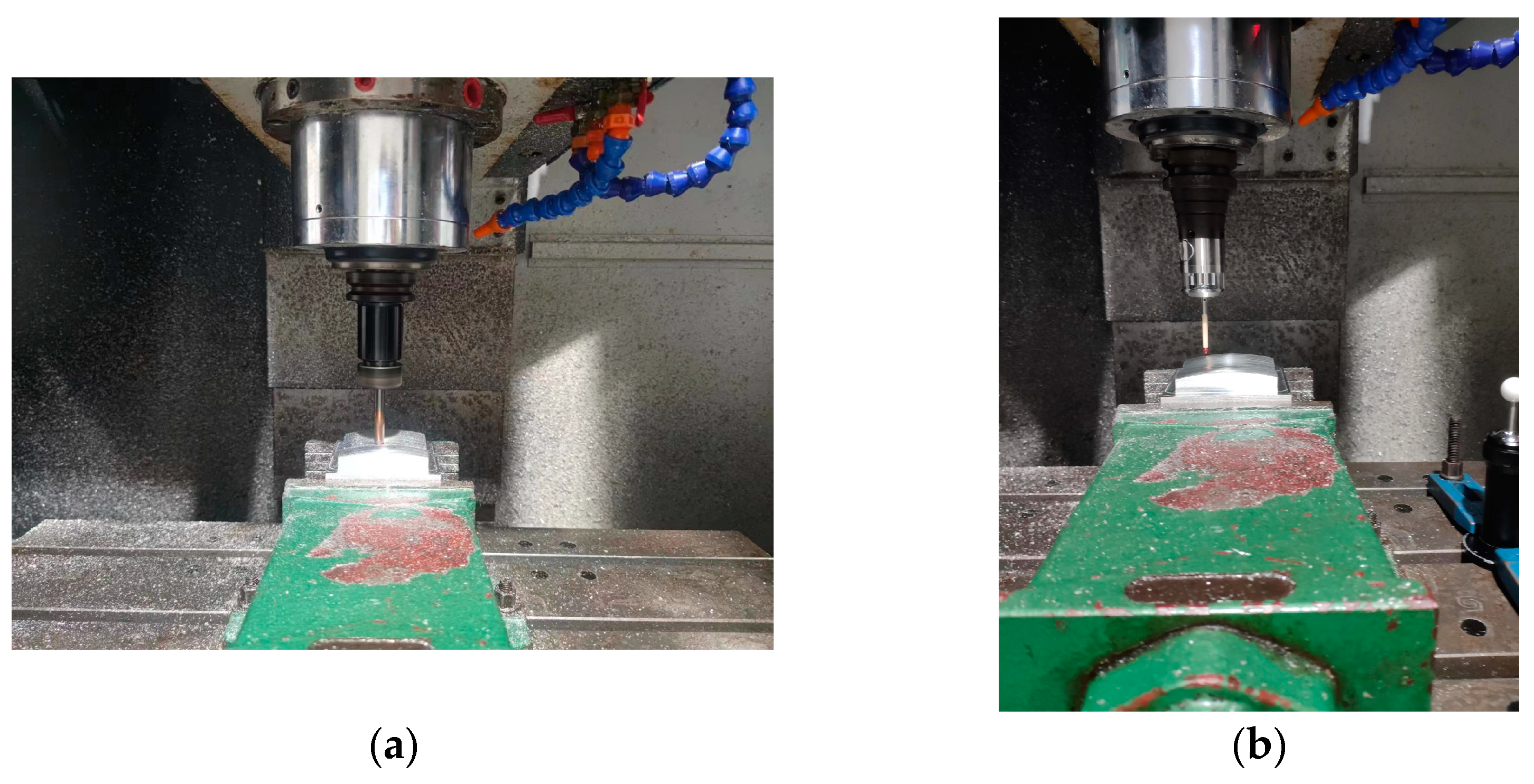
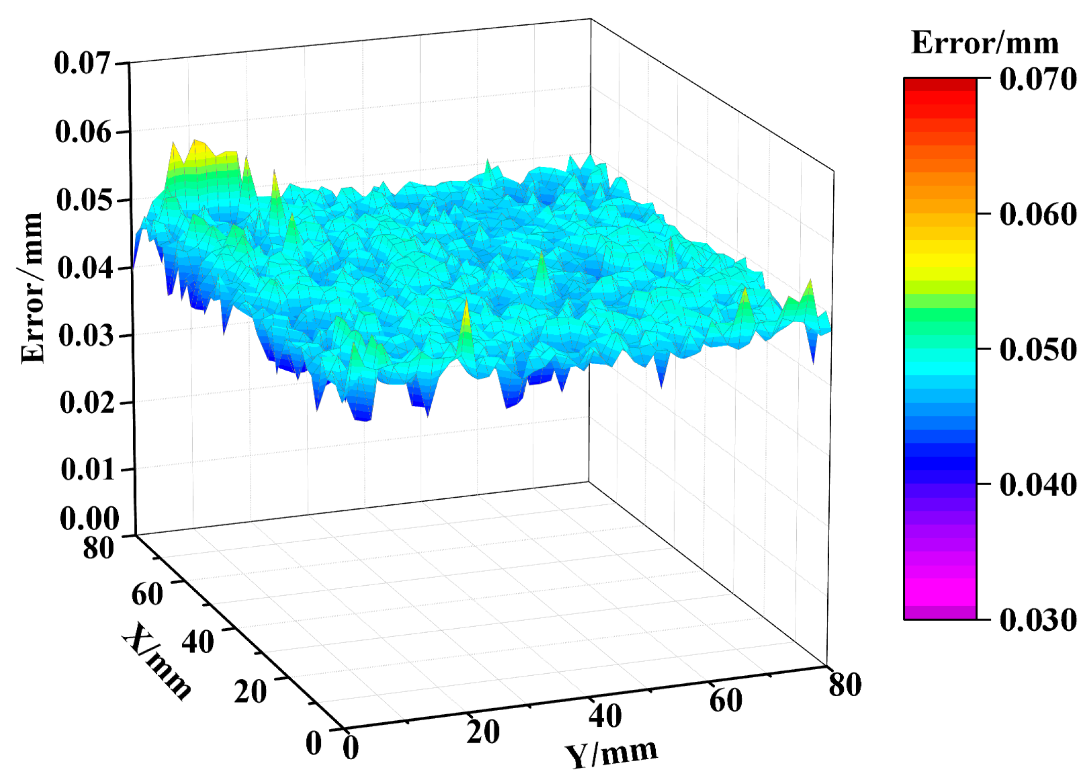
4.1. CNC Machining and On-Machine Measurement Processes

To verify the error compensation effect of the method proposed in this paper in the actual free-form surface machining process, an experiment on the machining of a free-form surface part was designed. On-machine inspection has been widely used in the manufacture of high-precision free-form surfaces or the machining of thin-walled parts because it does not require secondary clamping of the part and therefore does not introduce a secondary clamping error and also reduces time and effort [31]. The CNC machine used in the experiment was a VMC650E vertical machining center, and the inspection system was the IRP40.02 on-machine inspection system produced by Hexagon, with stylus end unidirectional positioning repeatability up to 0.0005 mm. First, the blank was cut, and, after semifinishing, the tool was removed, and the contact probe was installed. Generally, the greater the number is of measurement points on the free-form surface, the greater the reconstruction accuracy when reconstructing the machined surface [32]. The machining error after semifinishing, the original machining error, was obtained using on-machine measurements of the preset 2025 measurement points. The CNC machining process and the on-machine measurement process are shown in Figure 10.

According to the coordinate data of each measurement point obtained from the on-machine measurement, the original machining error of the free-form surface part was calculated, as shown in Figure 11.

4.2. Coarse-to-Fine Decomposition of the Original Machining Error Processes

First, the VMD algorithm was utilized for coarse decomposition of the original machining error, and the number of decomposition layers K was set to 7 according to the instantaneous frequency mean method. The decomposition results are shown in Figure 12.

The correlation coefficients between each IMF component in Figure 12 and the original machining error were calculated separately, and the corresponding correlation coefficients for each IMF component are shown in

Table 4. Correlation coefficients between each IMF component in VMD coarse decomposition and the raw machining error.

IMF Component	IMF1	IMF2	IMF3	IMF4	IMF5	IMF6	IMF7
correlation coefficient	0.4113	0.3893	0.2431	0.3775	0.2406	0.1158	0.3662

. The correlation coefficient thresholding was set to 0.3, and the corresponding correlation coefficients of each component were compared with the set thresholding to filter out the eligible IMF components, which were the IMF components containing systematic errors. As shown in Table 4, the components IMF1, IMF2, IMF4 and IMF7 met the screening conditions, which proves that they contained systematic errors, which were reorganized to obtain the coarse systematic error X₁.

Second, the coarse systematic error X₁ was used as the error to be decomposed, and it was adaptively decomposed using the EMD algorithm to obtain nine IMF components. Its decomposition results are shown in Figure 13.

The correlation coefficients between each IMF component in Figure 13 and the original machining error were calculated separately, and the corresponding correlation coefficients for each IMF component are shown in

Table 5. Correlation coefficients corresponding to each IMF in EMD.

IMF Component	IMF1	IMF2	IMF3	IMF4	IMF5	IMF6	IMF7	IMF8	IMF9
correlation coefficient	0.4688	0.3410	0.3160	0.3500	0.3369	0.1652	0.1511	0.1236	0.3650

.

By comparing the correlation coefficients corresponding to each of the IMF components with the thresholding set, it can be seen that the IMF components IMF1, IMF2, IMF3, IMF4, IMF5 and IMF9 were suitable for the screening conditions, and they were reorganized to obtain the systematic error X₂.

From the above decomposition process, it can be seen that components such as IMF3, IMF5 and IMF6 in the coarse decomposition process of the VMD algorithm were weakly correlated IMF components, and components such as IMF6, IMF7 and IMF8 in the decomposition process of the EMD algorithm were weakly correlated IMF components. All weakly correlated IMF components from the two decomposition processes were reorganized and decomposed using the wavelet thresholding method to obtain the residual systematic error X₃ contained in the weakly correlated IMF components. The residual systematic error X₃ and the systematic error X₂ obtained in the EMD process were reorganized to obtain the fine systematic error X₄ decomposed from the original machining error from coarse to fine, and its value and distribution are shown in Figure 14.

4.3. Compensation for the Fine System Error

On the surface of the free-form surface part, the machining errors corresponding to each measurement point were not the same. Therefore, to improve the error compensation effect of the part, the fine system error X₄ was compensated along the opposite direction of the outer normal vector of the measuring point, and the compensated coordinate data of the measuring point were obtained. The new machining surface was reconstructed according to the coordinates of the compensated measuring points, the corresponding NC code was generated for compensated machining, the tool path was checked without error and then imported into the CNC system of the machine tool and, finally, compensated machining was carried out. After the compensation machining was completed, the machining error of the free-form surface part was measured again using on-machine measurement techniques to obtain the machining error of the part after error compensation, and its value and distribution are shown in Figure 15.

The experimental data show that the maximum absolute machining error before compensation was 0.0580 mm, the maximum absolute machining error after compensation was 0.0159 mm, which was a 72.5% reduction, the mean absolute machining error before compensation was 0.0472 mm, and the mean absolute machining error after compensation was 0.0059 mm, which was an 87.5% reduction. By comparing the machining error measurement data before and after the compensation of the free-form surface part, it was found that, by utilizing the machining error decomposition method proposed in this paper to decompose the machining error first and then compensating for the decomposed systematic error, this machining error compensation method was able to improve its machining accuracy to a greater extent.

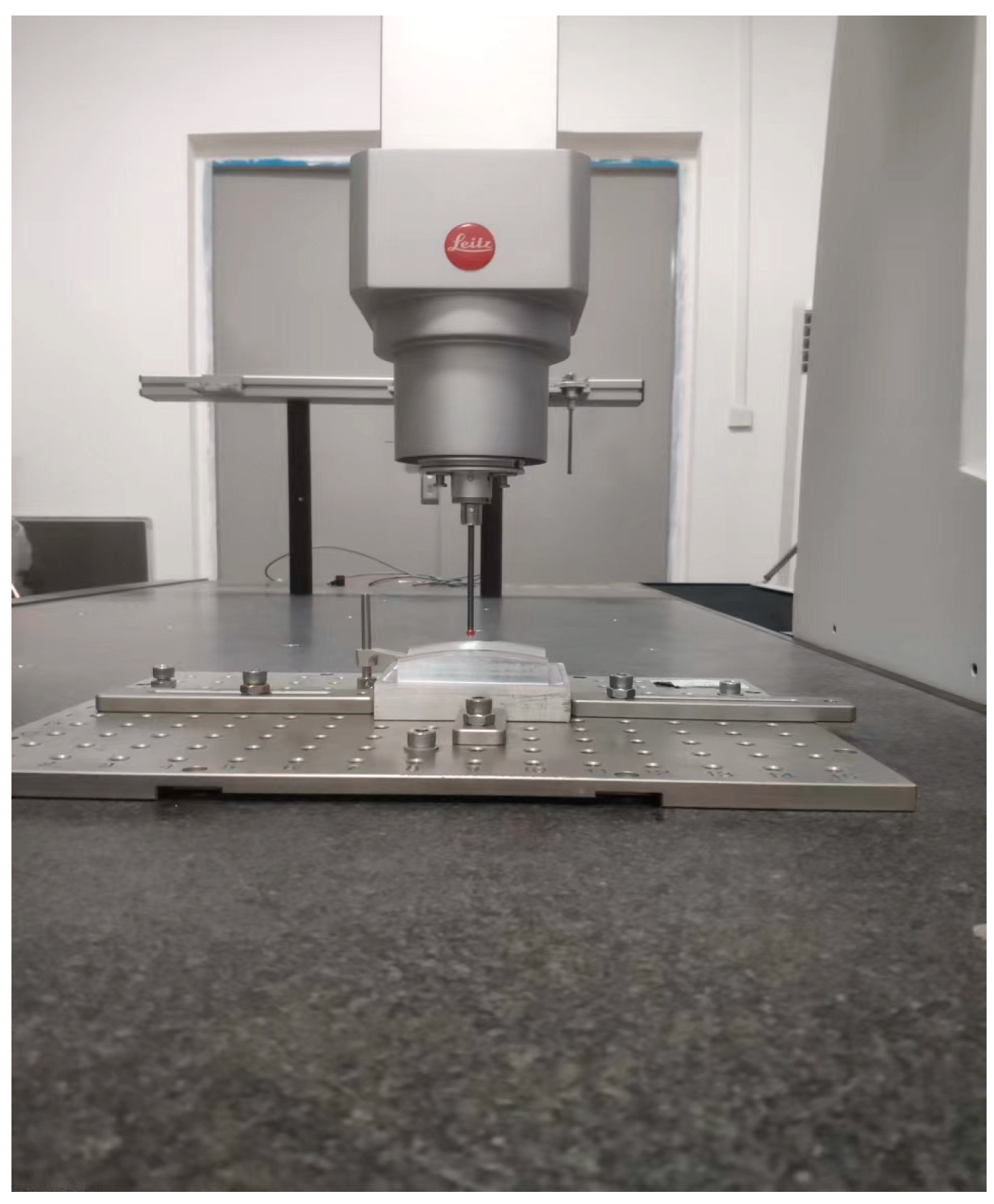
4.4. Measurement Experiment Using CMM

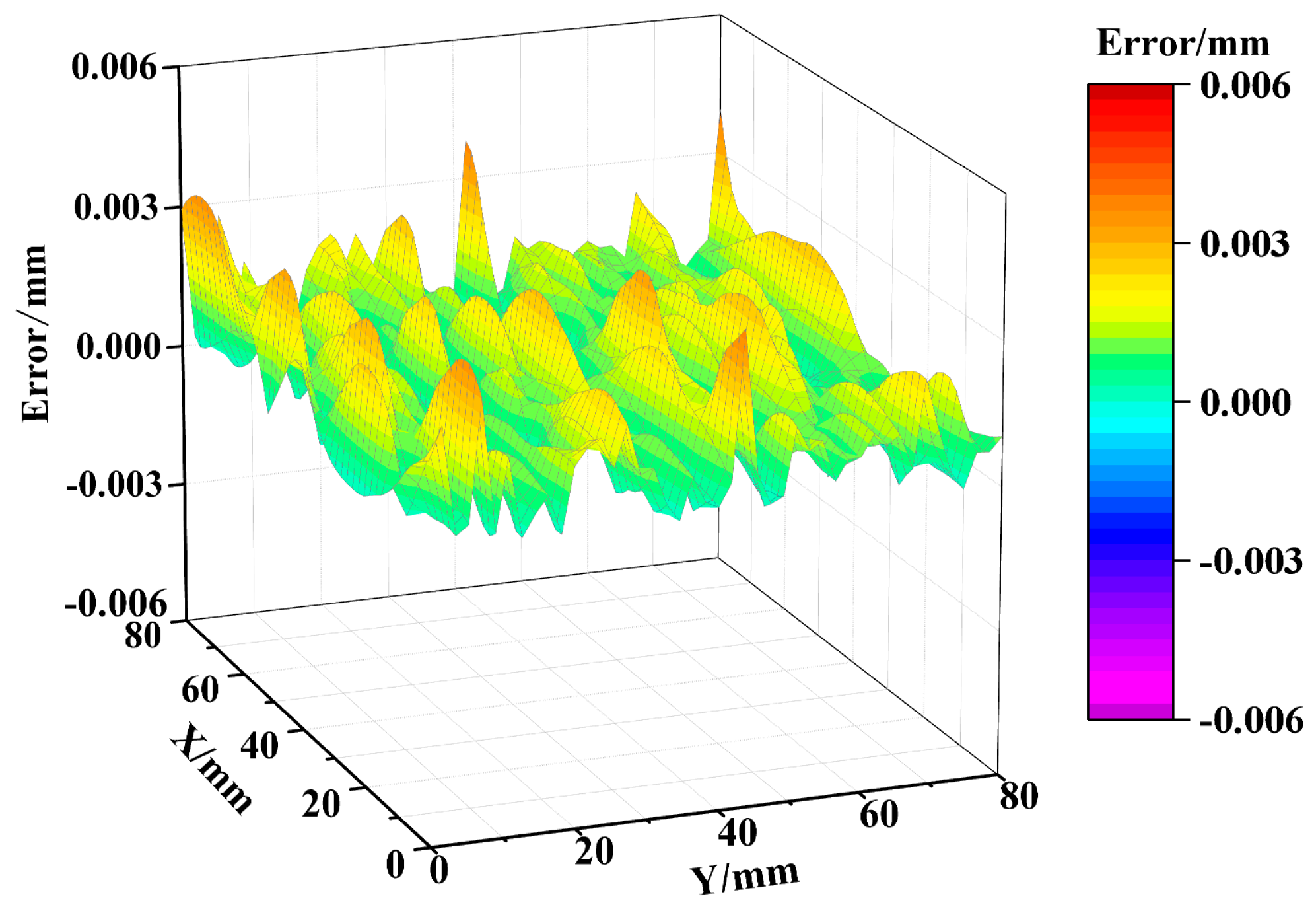
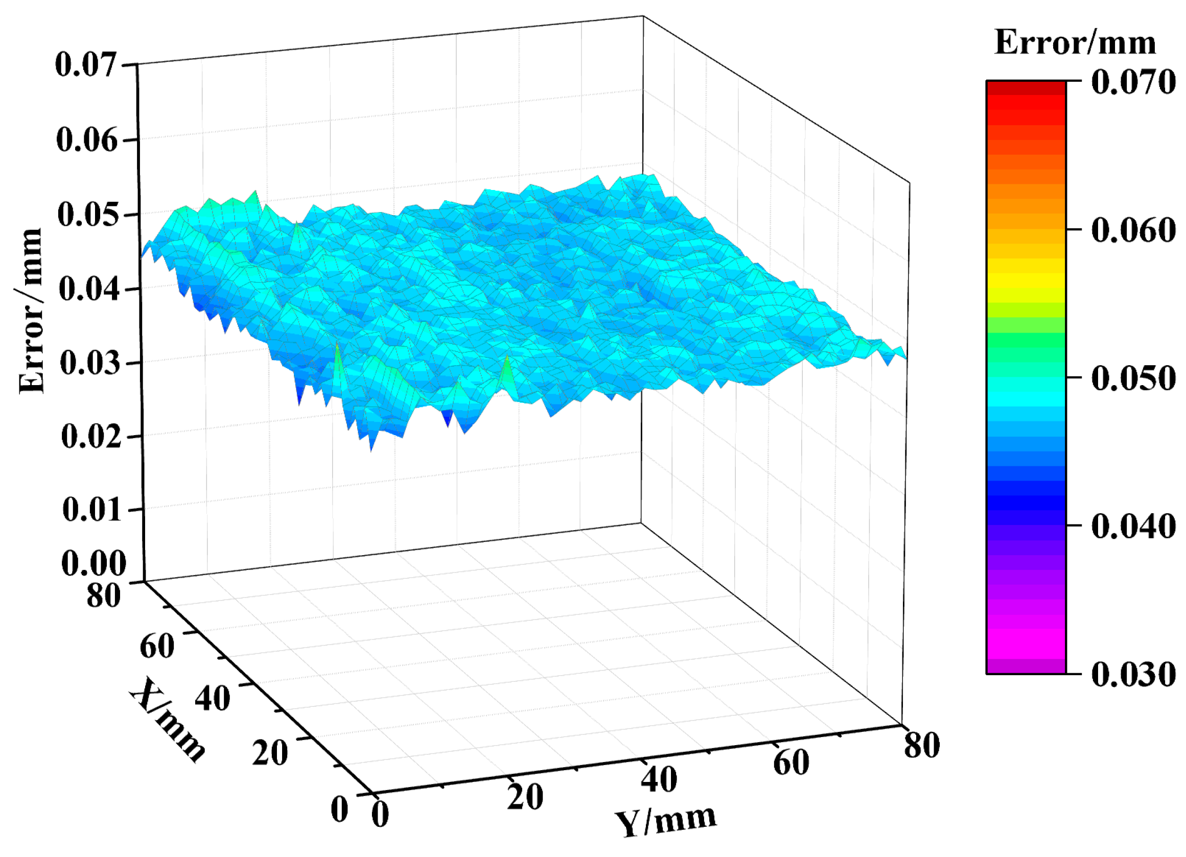
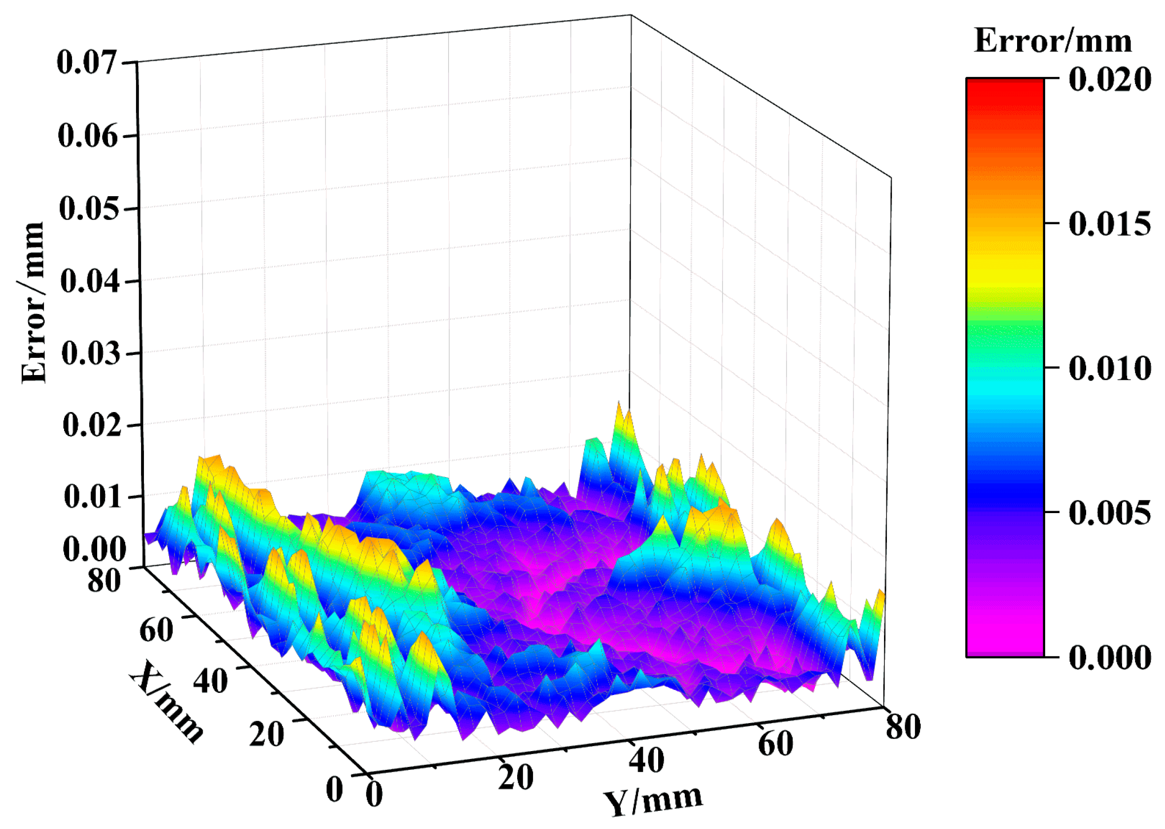
To verify the accuracy of the data obtained through on-machine measurement in this experiment, the machined free-form surface part was moved to a Hexagon (Hexagon manufacturing intelligence, Weinheim, Germany) ultrahigh-precision Leitz Reference HP CMM (PC-DMIS 2019 software, MPEE = 0.9 + L/400 μm) for the performance of the verification experiments, as shown in Figure 16.

An absolute average machining error of 0.0055 mm and a maximum absolute machining error of 0.0148 mm were obtained through CMM inspection, as shown in Figure 17.

The inspection results of the two different detection methods (on-machine measurement and CMM) are shown in

Table 6. Results of two different measurement methods (mm).

Detection Method	Before Machining Error Compensation		After Compensation for Machining Error
	Maximum absolute machining error	Mean absolute machining error	Maximum absolute machining error	Mean absolute machining error
On-machine measurement	0.0580	0.0472	0.0159	0.0059
CMM measurement	/	/	0.0148	0.0055

. By comparing the data in Table 6, it can be seen that the detection data of the on-machine measurements were very close to those of the CMMs, which indicates that the detection data obtained by the on-machine measurements have a certain credibility and accuracy.

To further verify the feasibility and effectiveness of the method proposed in this paper for free-form surface machining error compensation, two groups of comparative experiments were performed. Comparative group (1): machining error direct compensation method: First, the machining error of all the measurement points was obtained through on-machine inspection, then the machining error corresponding to each measurement point was directly used as the compensation value of the measurement point, and compensation was carried out along the opposite direction of its outer normal vector. Finally, the surface reconstruction method was utilized to compensate for the machining error. Comparative group (2): machining error decomposition and compensation method based on the VMD algorithm: First, the processing error was decomposed using VMD, then the IMF components containing systematic errors were screened out and reconstructed through correlation coefficient thresholding. Finally, the decomposed systematic errors were compensated for and processed using the surface reconstruction method. The experimental results are shown in

Table 7. Machining common error compensation using different compensation methods (mm).

Mode of Compensation	Before Machining Error Compensation		After Machining Error Compensation
	Maximum absolute machining error	Mean absolute machining error	Maximum absolute machining error	Mean absolute machining error
Machining error direct compensation method	0.0575	0.0435	0.0201	0.0124
Machining error decomposition and compensation method based on VMD algorithm	0.0594	0.0449	0.0186	0.0082
Coarse-to-fine machining error decomposition and compensation method	0.0580	0.0472	0.0159	0.0059

.

4.5. Data Analysis

In comparative group (1), the maximum absolute machining error of the free-form surface part before compensation was 0.0575 mm, and the mean absolute machining error was 0.0435 mm, which was a 24.3% reduction. However, the maximum absolute machining error after compensation was 0.0201 mm, and the mean absolute machining error was 0.0124 mm, which represents a reduction of 71.49% in the mean absolute machining error. In comparative group (2), the maximum absolute machining error of the free-form surface part before compensation was 0.0594 mm, and the mean absolute machining error was 0.0449 mm. On the other hand, the maximum absolute machining error after compensation was 0.0186 mm, and the mean absolute machining error was 0.0082 mm, which was a 24.4% reduction in the maximum absolute machining error and an 81.73% reduction in the mean absolute machining error. In the compensation method proposed in this paper, the maximum absolute machining error of the free-form surface part before compensation was 0.0580 mm and the mean absolute machining error was 0.0472 mm, while the maximum absolute machining error after compensation was 0.0159 mm and the mean absolute machining error was 0.0059 mm, which represents a 72.5% reduction of the maximum absolute machining error and an 87.50% reduction of the average absolute machining error.

After compensating for the machining error of the free-form surface part by using the three compensation methods, the machining accuracies greatly improved. The compensation method proposed in this chapter was the most effective, the second most effective was comparative group (2) and comparative group (1) was the least effective in terms of compensation. The main reasons for this were as follows:

• All three methods compensate for the error of each measurement point sequentially, and use the surface reconstruction method to make the tool trajectory in the compensated machining smoother, and thereby improve the machining accuracy of the part.
• Because the random error was more random, it was not easy to compensate for, and, because the processing error was relatively small, direct processing error compensation rather than only the system error compensation effect was good.
• According to the experimental data in Table 3 and Table 7, the more complete and accurate the decomposed system error was, the better the compensation effect. Compared with the VMD algorithm, the coarse-to-fine machining error decomposition method proposed in this paper was superior in its ability to decompose and compensate for machining errors.

Therefore, through the machining error compensation experiment of the free-form surface part, it was proven that the free-form surface machining error decomposition and compensation method from coarse to fine can improve the machining accuracy of the free-form surface part to a larger extent, and the method has a certain degree of advancement, accuracy and effectiveness.

5. Conclusions

In this paper, a method to decompose and compensate for the machining error from coarse to fine was proposed. First, the machining error was obtained through on-machine measurement. Second, VMD-EMD was combined with the wavelet thresholding method, and the IMF components containing systematic errors were screened out by setting the appropriate correlation coefficient thresholding to obtain the systematic error contained in the machining error. Finally, the machining surface was reconstructed according to the decomposed systematic error, and the corresponding compensating tool path was generated to compensate for the systematic error to enhance the free-form machining accuracy of the free-form surface part.

In actual CNC machining experiments, after the machining error was compensated for by this method, the maximum absolute error decreased from 0.058 mm to 0.0159 mm, the mean machining error decreased from 0.0472 mm to 0.0059 mm, which represents a 72.5% reduction of the maximum absolute machining error, and the mean absolute machining error decreased by 87.5%. Notably, the method has better machining error decomposition and compensation ability and can greatly improve the machining accuracy of free-form surface parts, which has certain research significance.

References

1. Poniatowska, M. Free-form surface machining error compensation applying 3D CAD machining pattern model. Comput. Aided Des. 2015, 62, 227–235. [Google Scholar] [CrossRef]
2. He, J.M.; Luo, J.X.; Zhong, W.J.; Liu, Z.L.; Ding, K. Error source analysis and compensation method of CNC machine tools. Mod. Manuf. Technol. Equip. 2020, 2, 131–132. [Google Scholar] [CrossRef]
3. Zhang, Z.; Jiang, F.; Luo, M.; Wu, B.; Zhang, D.; Tang, K. Geometric error measuring, modeling, and compensation for CNC machine tools: A review. Chin. J. Aeronaut. 2024, 37, 163–198. [Google Scholar] [CrossRef]
4. Ge, G.Y.; Du, Z.C.; Feng, X.B.; Yang, J. An integrated error compensation method based on on-machine measurement for thin web part machining. Precis. Eng. 2020, 63, 206–213. [Google Scholar] [CrossRef]
5. Liu, Y.; Wan, M.; Xing, W.J.; Xiao, Q.B.; Zhang, W.H. Generalized actual inverse kinematic model for compensating geometric error in five-axis machine tools. Int. J. Mech. Sci. 2018, 145, 299–317. [Google Scholar] [CrossRef]
6. Li, Z.H.; Feng, W.L.; Yang, J.G.; Huang, Y. An investigation on modeling and compensation of synthetic geometric error on large machine tools based on moving least squares method. Proc. Inst. Mech. Eng. Part B J. Eng. Manuf. 2018, 232, 412–427. [Google Scholar] [CrossRef]
7. Msaddek, E.B.; Baili, M.; Bouaziz, Z.; Dessein, G. Compensation of machining error of B spline and C spline. Int. J. Adv. Manuf. Technol. 2018, 97, 4055–4064. [Google Scholar] [CrossRef]
8. Fu, G.Q.; Zhang, L.; Fu, J.Z.; Gao, H.; Jin, Y. F test-based automatic modeling of single geometric error component for error compensation of five-axis machine tools. Int. J. Adv. Manuf. Technol. 2018, 94, 4493–4505. [Google Scholar] [CrossRef]
9. Wu, B.H.; Yin, Y.J.; Zhang, Y.; Luo, M. A new approach to geometric error modeling and compensation for a three-axis machine tool. Int. J. Adv. Manuf. Technol. 2019, 102, 1249–1256. [Google Scholar] [CrossRef]
10. Chen, Y.P.; Tang, H.; Tang, Q.C.; Zhang, A.; Chen, D.; Li, K. Machining error decomposition and compensation of complicated surfaces by EMD method. Measurement 2018, 116, 341–349. [Google Scholar] [CrossRef]
11. Lin, Z.X.; Tian, W.J.; Zhang, D.J.; Gao, W.; Wang, L. A method of geometric error identification and compensation of CNC machine tools based on volumetric diagonal error measurements. Int. J. Adv. Manuf. Technol. 2023, 124, 51–68. [Google Scholar] [CrossRef]
12. Zhang, Y.; Zhang, D.H.; Wu, B.H. An approach for machining allowance optimization of complex part with integrated structure. J. Comput. Des. Eng. 2015, 2, 248–252. [Google Scholar] [CrossRef]
13. Li, Y.; Zhao, J.; Ji, S.J. Thermal positioning error modeling of machine tools using a bat algorithm-based back propagation neural network. Int. J. Adv. Manuf. Technol. 2018, 97, 2575–2586. [Google Scholar] [CrossRef]
14. Reddy, T.N.; Shanmugaraj, V.; Vinod, P.; Krishna, S.G. Real-time thermal error compensation strategy for precision machine tools. Mater. Today Proc. 2020, 22, 2386–2396. [Google Scholar] [CrossRef]
15. Wei, J.; Jiang, L.; Liang, B. Geometric error compensation method of five-axis CNC machine tool based on improved genetic algorithm. J. Phys. Conf. Ser. 2024, 2825, 012029. [Google Scholar] [CrossRef]
16. Zha, J.; Villarrazo, N.; de Pisson, G.M.; Li, Y.; Zhang, H.; de Lacalle, L.N.L. An accuracy evolution method applied to five-axis machining of curved surfaces. Int. J. Adv. Manuf. Technol. 2023, 125, 3475–3487. [Google Scholar] [CrossRef]
17. Zhang, L.; Zhang, Z.S.; Zhou, Y.F.; Dai, M.; Shi, J.F. Stream of variation modeling and analysis for manufacturing processes based on a semi-parametric regression model. J. Mech. Eng. 2013, 49, 180–185. [Google Scholar] [CrossRef]
18. Wang, G.; Li, W.L.; Tong, G.; Pang, C.-T. Improving the machining accuracy of thin-walled part by online measuring and allowance compensation. Int. J. Adv. Manuf. Technol. 2017, 92, 2755–2763. [Google Scholar] [CrossRef]
19. Lee, W.; Lee, Y.; Wei, C.C. Automatic error compensation for free-form surfaces by using on-machine measurement data. Appl. Sci. 2019, 9, 3073. [Google Scholar] [CrossRef]
20. Chen, Y.P.; Jin, L.; Lu, H.Y.; Feng, Z.J.; Chen, Y.H. Application of spatial statistical analysis in decomposition of machining errors for free-form surfaces. J. Beijing Inst. Technol. 2017, 37, 260–266. [Google Scholar] [CrossRef]
21. Liu, R.N.; Xin, Y.Z.; Li, Y. Dynamic signature verification method based on Pearson correlation coefficient. Chin. J. Sci. Instrum. 2022, 43, 279–287. [Google Scholar] [CrossRef]
22. Asuero, A.G.; Sayago, A.; González, A.G. The correlation coefficient: An overview. Crit. Rev. Anal. Chem. 2006, 36, 41–59. [Google Scholar] [CrossRef]
23. Cohen, J. Statistical Power Analysis for the Behavioral Sciences; Routledge: New York, NY, USA, 1988. [Google Scholar] [CrossRef]
24. Dragomiretskiy, K.; Zosso, D. Variational mode decomposition. IEEE Trans. Signal Process. 2014, 62, 531–544. [Google Scholar] [CrossRef]
25. Zhang, X.; Miao, Q.; Zhang, H.; Wang, L. A parameter-adaptive VMD method based on grasshopper optimization algorithm to analyze vibration signals from rotating machinery. Mech. Syst. Signal Process. 2018, 108, 58–72. [Google Scholar] [CrossRef]
26. Huang, N.E.; Shen, Z.; Long, S.R.; Wu, M.C.; Shih, H.H.; Zheng, Q.; Yen, N.-C.; Tung, C.C.; Liu, H.H. The empirical mode decomposition and the Hilbert spectrum for nonlinear and non-stationary time series analysis. Proc. R. Soc. Lond. Ser. A Math. Phys. Eng. Sci. 1998, 454, 903–995. [Google Scholar] [CrossRef]
27. Song, X.J.; Sun, H.W.; Zhan, L.W. Novel complete ensemble EMD with adaptive noise-based hybrid filtering for rolling bearing fault diagnosis. J. Vibroeng. 2019, 21, 1845–1858. [Google Scholar] [CrossRef]
28. Lu, Q.; Pang, L.X.; Huang, H.Q.; Shen, C.; Cao, H.; Shi, Y.; Liu, J. High-G calibration denoising method for high-G MEMS accelerometer based on EMD and wavelet thresholding. Micromachines 2019, 10, 134. [Google Scholar] [CrossRef] [PubMed]
29. Xie, B.; Xiong, Z.Q.; Wang, Z.J.; Zhang, L.; Zhang, D.; Li, F. Gamma spectrum denoising method based on improved wavelet thresholding. Nucl. Eng. Technol. 2020, 52, 1771–1776. [Google Scholar] [CrossRef]
30. Chang, Y.; Bao, G.Q.; Cheng, S.K.; He, T.; Yang, Q. Improved VMD-KFCM algorithm for the fault diagnosis of rolling bearing vibration signals. IET Signal Process. 2021, 15, 238–250. [Google Scholar] [CrossRef]
31. Li, S.L.; Zeng, L.; Feng, P.F.; Li, Y.; Xu, C.; Ma, Y. Accurate compensation method for probe pre-travel error in on-machine inspections. Int. J. Adv. Manuf. Technol. 2019, 103, 2401–2410. [Google Scholar] [CrossRef]
32. Cheng, X.; Liu, X.P.; Feng, P.F.; Zeng, L.; Jiang, H.; Sun, Z.; Zhang, S. Efficient adaptive sampling methods based on deviation analysis for on-machine inspection. Measurement 2022, 188, 110497. [Google Scholar] [CrossRef]
Figure 1. Flowchart of coarse-to-fine machining error decomposition.
Applsci 14 09044 g001
Figure 2. Modeling of the free-form surface workpiece and placement of the measurement points.
Applsci 14 09044 g002
Figure 3. Simulation systematic error.
Applsci 14 09044 g003
Figure 4. Random error of the simulation.
Applsci 14 09044 g004
Figure 5. Machining error of the simulation.
Applsci 14 09044 g005
Figure 6. Coarse decomposition of the simulated machining error via the VMD algorithm.
Applsci 14 09044 g006
Figure 7. EMD algorithm to decompose the coarse systematic error X1.
Applsci 14 09044 g007
Figure 8. Fine systematic error X4.
Applsci 14 09044 g008
Figure 9. Error between the simulated systematic error and the fine systematic error X4.
Applsci 14 09044 g009
Figure 10. Free-form surface part (a) CNC machining process; (b) on-machine measurement process.
Applsci 14 09044 g010
Figure 11. Original machining error on the free-form surface part.
Applsci 14 09044 g011
Figure 12. Coarse decomposition of the original machining error via VMD.
Applsci 14 09044 g012
Figure 13. EMD algorithm for the decomposition of coarse systematic error.
Applsci 14 09044 g013
Figure 14. Fine system error X4.
Applsci 14 09044 g014
Figure 15. Machining error of the free-form surface part after error compensation.
Applsci 14 09044 g015
Figure 16. CMM inspection process.
Applsci 14 09044 g016
Figure 17. CMM inspection results.
Applsci 14 09044 g017