Article

Spatial Heterogeneity of Soil Nutrient in Principal Paddy and Cereal Production Landscapes of Fengtai County within the Huai River Basin, Eastern China

1
School of Earth and Environment, Anhui University of Science and Technology, Huainan 232001, China
2
School of Chemistry and Chemical Engineering, South China University of Technology, Guangzhou 510641, China
3
Xi’an Center of Mineral Resources Survey, China Geological Survery, Xi’an 710100, China
4
School of Earth Resources and Materials Engineering, RWTH Aachen University, 52062 Aachen, Germany
*
Author to whom correspondence should be addressed.
First author.
Appl. Sci. 2024, 14(19), 9087; https://doi.org/10.3390/app14199087
Submission received: 22 July 2024 / Revised: 16 September 2024 / Accepted: 23 September 2024 / Published: 8 October 2024

Abstract

:
The problem of cultivated land soil quality in the Huaihe River Basin has become increasingly prominent. How to accurately and quantitatively evaluate the soil quality of regional cultivated land and realize its efficient use has become an urgent problem. In order to explore the spatial autocorrelation and variation in soil nutrients in cultivated land in the plain of Fengtai County in the Huaihe River Basin, a total of 306 soil samples and mature wheat samples were collected in the study area to analyze soil pH, total nitrogen (TN), available nitrogen (AN), available phosphorus (AP), available potassium (AK) and slow-release potassium (SK) content and wheat biomass, and combined with geostatistical methods and GIS technology. The Kriging interpolation method and Moram‘s I index method were systematically analyzed. Principal component analysis (PCA) and Pearson correlation analysis were used to establish the minimum data set (MDS) of soil quality, which was used to calculate the soil quality index (SQI) and determine the key factors affecting soil quality. The results showed that the soil pH was in weak variation, and the other nutrient indexes were in medium variation. The spatial variability of soil-available potassium nutrients was affected by random factors such as human activities and structural factors such as soil parent materials. The spatial autocorrelation of organic matter, total nitrogen, alkali-hydrolyzable nitrogen, available phosphorus, available potassium and mitigation potassium was weak, which was mainly affected by random factors such as human activities. An unequivocal positive spatial nexus was discerned across all nutrients. Cumulatively, the nutrient dispersion across the investigated territory was somewhat diffuse, manifesting in a mosaic pattern with pronounced zonal nutrient allocation disparities in the meridional, median, and septentrional segments. An explicit latitudinal dichotomy delineating zones of nutrient opulence and paucity was also observed. These insights can pave the way for tailored fertilization strategies and judicious pedological stewardship in Fengtai County.

1. Introduction

Food is indubitably the cornerstone of human existence. As the worldwide population exhibits an unremitting ascent, the burgeoning discrepancy between food supply and demographic demand emerges as a preeminent conundrum, more so in the context of developing nations [1]. Soil, as a partially renewable resource, emerges as the linchpin for food production. Beyond merely dispensing indispensable nutrients imperative for crop cultivation, soils have a salient role in underpinning broader human advancement [2]. Soil ecosystem service is the terminal of the soil ecosystem formed under the influence of human value orientation, and it is the direct contribution of the ecosystem to human income. Soil function is similar to the intermediate process of serving soil and exerting ecosystem service function [3]. Through an astute grasp of soil nutrient profiles, we can judiciously administer fertilizers, adopt congruent crop rotations, amplify fertilizer assimilation efficiencies, augment soil physicochemical attributes, and maintain a harmonized nutrient equilibrium within soils [4,5]. The evaluation system of soil quality can be determined by using reverse thinking to find the characteristics of soil quality. Soil quality, as a measure of the degree to which soil plays its role in its ecosystem, affects the productivity and sustainability of agriculture [3]. The spatial heterogeneity of soil nutrients is orchestrated by determinate variables encompassing topography, climatic parameters, and the lithological lineage of the soil [6]. In juxtaposition, stochastic human interventions—such as fertilization methodologies, tillage protocols, and irrigation paradigms—also leave their imprint [7,8]. Delineating the spatial dispersal nuances of soil nutrients and grasping their extant state is of paramount significance for escalating crop outputs and fostering an agrarian paradigm rooted in sustainability; it can also map the ability of soil to provide ecosystem services from the side.
Regional discernment of soil nutrient spatial dynamics forms the bedrock of their scientific oversight and judicious management [9]. Geostatistical methodologies, appreciating the spatial autocorrelation inherent in variables, bridge the void of conventional statistical models that often overlook spatial nuances [10]. Antecedent scholarly endeavors have delved into the spatial contours and intricate heterogeneity of soil nutrients across diverse landscapes, harnessing the synergies of geostatistical tools allied with Geographic Information Systems (GIS) technology [11]. Smith et al. employed the multi-index Kriging method combined with GIS technology for automated assessment and dynamic monitoring of soils [12]. Yaolin Liu and colleagues utilized a stratified regression Kriging method based on a geodetector, wherein soil and land-use types were treated as categorical variables and the percentage of land use as a continuous variable. Their research yielded nutrient content maps with high spatial heterogeneity [13]. Mishra et al. analyzed the geospatial framework data set of more than 2700 soil profiles and environmental variables in the permafrost region of the northern hemisphere, generated a spatially explicit SOC storage estimation in the permafrost region, and quantified the spatial heterogeneity. It is identified that soil moisture and elevation are the main topographic control factors of SOC storage, while surface temperature (polar region) and precipitation (Qinghai–Tibet Plateau) are significant climate control factors [14]. Chen and his team obtained soil sample data from different years and, using the semivariogram method and Kriging interpolation, studied the spatiotemporal variation characteristics of soil nutrients [15]. Wang et al. leveraged geostatistical methods and the inverse distance weighting method to analyze the spatial distribution of soil nutrients in China’s Pearl River Delta region. Their findings showed that the overall spatial distribution of readily available potassium and total nitrogen increased from the northeast to the southwest, while the distribution of available potassium and available silica was higher in the northeast than in the southwest [16]. This research offers insights into region-specific crop selection. Yan and his team, focusing on the Nanxiong Basin in South China as a case study, employed geostatistical methods to analyze the spatial variation characteristics of soil pH values. Their results identified that land-use patterns and topographical factors were the primary and secondary contributors, respectively, to the pH values of the soil in the area [17]. In recent years, most studies examining the spatial variation characteristics of soil nutrients have been based on low-density sampling data over larger scales. Moreover, the nutrient indices researched for the soil in China’s Huai River Basin region have been relatively singular, with comprehensive comparative studies between nutrients being rare. This has made it challenging to offer practical guidance for modern precision agriculture production and the prevention and control of non-point source pollution.
This study is centered on Fengtai County, situated in the Huai River Basin of China, which is represented as a grain-producing region. Soil nutrient data from concurrent sample collections were analyzed. Using ArcMap 10.8, the best semivariogram model parameters were determined to gauge spatial autocorrelation. The global Moran’s I index was utilized to verify the relevance of soil nutrient autocorrelation. Based on the optimal model, the Ordinary Kriging interpolation was employed to craft nutrient content spatial distribution maps. The local Moram’s I index was also utilized to fashion LISA cluster maps. This approach is characterized by the marriage of geostatistical methods with GIS technology. Subsequently, the author investigated the wheat yield of typical crops under the same sampling point in the second year, analyzed the correlation between yield and soil nutrients, and used PCA principal component analysis to score the overall soil quality of Fengtai County, and determined the influencing factors that restrict the soil quality in this area. The research results of the combination of geostatistics and GIS technology were further demonstrated to provide theoretical support for the rational fertilization of soil in this area, the precise development of agriculture, and the consideration of soil ecological service functions.

2. Materials and Methods

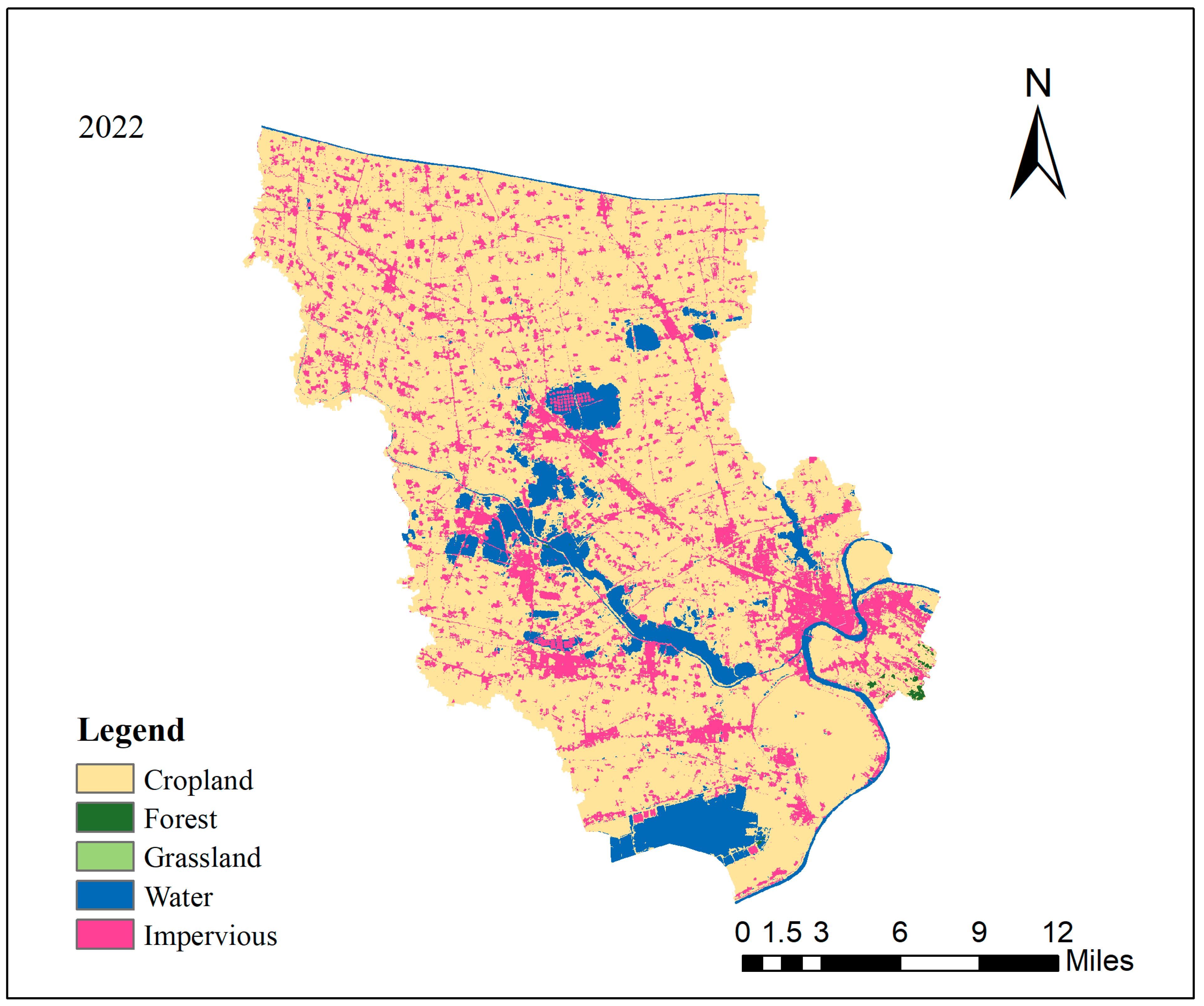
2.1. Study Area Description

Situated in central Anhui Province, the study area lies in the midsection of the Huai River. It is geographically positioned between 116°52′02.1″ E and 116°56′19.0″ E longitude, and 32°34′45.5″ N and 32°36′38.9″ N latitude. It is located in the transition zone between the subtropical zone and the warm temperate zone. The climate characteristics are obvious, the four seasons are distinct, the annual average temperature is 15.3 °C, the annual average frost-free period is 224 days, and the precipitation in the four seasons is relatively average. The annual precipitation is 937.2 mm, and the average annual sunshine is 2609.9 h. Due to the superior light conditions, abundant heat, moderate precipitation, and long frost-free period, it is suitable for planting food crops and economic crops such as soybeans, wheat, rice, and rapeseed. The study area is the Jianghuai Plain area, and the terrain is a low hilly area with little ups and downs. According to the soil classification of WRB, the soil types of sampling sites in the study area include Gleyic Fluvisols, Haplic Fluvisols, Ferric Luvisol, and Anthraqui-Stagnic Luvisol. The physical properties of the typical soil in the study area are shown in Table 1, and the soil texture of sampling points is shown in Figure 1. Most of the sampling points are A-B-C and A-B-C-D. The color of the whole section is yellowish brown to brown, the clay plate appears above 20 cm, and the texture is heavy soil to clay. From massive to prismatic structure, there are new bodies such as iron–manganese binding and dark film, and their number is increasing from top to bottom.

2.2. Sample Collection and Analysis

Based on the way of land use, the sampling units are divided into administrative village-level units and cultivated land area, and the sampling principle of random distribution of the system is combined with the latest GF satellite image data to adjust the point error. Finally, the sampling point is determined by an on-site field survey. A total of 306 sampling points were set in the study area (Figure 2), and the elevation of the study area is shown in Figure 3. These sampling points were located in the rice–wheat rotation field, and GPS was carried out to record the location of the sampling points, and multi-point mixed sampling was carried out according to the diagonal method (The specific distribution of cropland land in the study area can be referred to Figure 4). The sampling time was April 2023, and the five-point sampling method was used to set up 1 × 1 m standard plots with each sampling point as the center, with a total of 306 plots. Five sampling points (diameter of 0.15 m) were set along the double diagonal direction in the plot, and the profile analysis (0–100 cm) was carried out at the center of the plot. The ring knife method was used to sample (0–15 cm, 15–30 cm, 30–100 cm), and each layer was repeated three times as a physical property test sample. In addition, the topsoil (0–20 cm) of the five sampling points in the plot was mixed, and the excess samples were discarded by the quartering method. The final sampling amount was 1–2 kg. We removed the foreign bodies such as stone particles and plant roots contained in the soil, put them in plastic bags, attached labels, recorded the number, coordinates, profile depth and other information, and brought them back to the laboratory for analysis. In May 2024, a 1 × 1 m plot was set up for 306 sampling points recorded by GPS, and all mature wheat on the plot was harvested and brought back to the laboratory for analysis.
The collected soil samples were subjected to air drying. These dried samples were then ground and sieved through a 2 mm mesh. The sieved soil samples were mixed thoroughly and used for the determination of soil nutrient indicators. Soil physicochemical property indicators were determined following standard methods of China [18]. The pH of the soil was measured using a pH meter with a soil-to-water ratio of 2.5:1. The organic matter in the soil was determined using the potassium dichromate external heating method. Total nitrogen in the soil was determined by the semi-micro Kjeldahl method. Available phosphorus in the soil was determined by the sodium bicarbonate extraction-antimony molybdenum spectrophotometry method. Available K in the soil was determined using atomic absorption spectrophotometry, while slow-release potassium was determined using the hot nitric acid extraction-flame photometry method.
The aboveground part of wheat was divided into three parts: stem and leaf, grain and glume + rachis (referred to as glume) and dried naturally. After weighing, it was placed in an oven at 65 °C to constant weight. The weight was weighed and the water content of the air-dried sample was calculated, and then the dry matter accumulation of all wheat in the unit plot was calculated.

2.3. Statistical and Geostatistical Methods

2.3.1. Geostatistical Analysis

The semivariogram is a commonly used method for analyzing the spatial variability of soil nutrients. It is a core concept in geostatistics and can reveal the extent to which randomness and structural factors influence regionalized variables [19]. Its variogram formula [20] is as follows:
γ ( h ) = 1 2 N ( h ) i = 1 N ( h ) ( Z i Z i + h ) 2
where γ(h) represents the semivariance for a spatial distance of h, N(h) represents the number of sample pairs at a spatial distance of h, and Z i and Z i + h represent the actual values of the variable at points i and i + h, respectively.
The semivariogram consists of the nugget value (C0), sill value (C0 + C), and range a. Common semivariogram models include the spherical model, Gaussian model, linear model, and exponential model.

2.3.2. Spatial Autocorrelation Analysis

The dependence of soil properties in geographic space on the observed values in adjacent regions, known as spatial autocorrelation [21], can be represented by the global Moran’s I index (IN). The formula for its computation is as follows:
I N = N i = 1 N j = 1 N W i j ( x i x ¯ ) ( x j x ¯ ) ( i = 1 N j = 1 N W i j ) i = 1 N ( x i x ¯ ) 2
where N is the number of samples, xi and xj are the observed values at locations i and j in space, respectively, Wij denotes the spatial weight, and x ¯ is the sample mean.
The range of IN values lies between −1 and 1. Values less than 0 indicate a negative correlation, while those greater than 0 suggest a positive correlation. The larger the absolute value, the more pronounced the autocorrelation. An IN value of 0 indicates no correlation, implying a random spatial distribution. The significance level of IN is tested using the following equation:
Z = [ I N E ( I N ) ] / var ( I N )
where Z is the statistic to test the significance of the IN index, E(IN) represents the expected value, and var(IN) is the variance. Through the Z-score, its significance can be verified. At a confidence level of 0.01, a |Z| value of ≥1.96 indicates significant spatial autocorrelation, while a |Z| value of ≥2.58 points to highly significant spatial autocorrelation.

2.3.3. Spatial Clustering Analysis

Spatial clustering analysis is based on the local Moram’s I index to reflect local spatial autocorrelation. Its computation formula is:
I i = N ( x i x ¯ ) j = 1 N W j i ( x j x ¯ ) i = 1 N ( x i x ¯ ) 2
where the variable definitions are consistent with Equation (2).
The local Moram’s I index divides the study area into 5 scenarios: ① Insignificant type: No significant spatial correlation, showing a random distribution. ② High–High type: Regions with clustered high values. ③ High–Low type: Areas of low values surrounding regions of high values. ④ Low–High type: Areas of high values surrounding regions of low values. ⑤ Low–Low type: Regions with clustered low values. LISA (Local Indicators of Spatial Association) cluster maps can represent the correlation of soil properties in localized areas.

2.4. Soil Quality Assessment

2.4.1. Minimum Data Set Construction

Considering the frequency and representativeness of soil index selection and experimental conditions in previous studies [22], the seven soil nutrient indexes were determined as TDS. The results of KMO sampling and Bartlett’s sphericity test show that the KMO value is 0.784 > 0.6, and the sphericity test is 0, which is significant, indicating that the principal component analysis can be carried out based on the selected indicators. MDS was screened by the PCA method. Based on the data of principal component analysis, we selected the principal components with eigenvalues greater than or equal to 1, and selected the part with the maximum factor load within 10% from each principal component as the evaluation standard of high load according to the size of factor load. If the principal component contains only one high-load index, then this index will be included in the MDS data set; if there are multiple indicators related to high load, Pearson correlation analysis can be used to determine the specific indicators of soil [23]. If there is no correlation between these indicators, then all indicators should be stored in MDS; otherwise, only the indicators with the largest load should be selected to join MDS [24].

2.4.2. Construction of Soil Quality Scoring Method

After the TDS and MDS indexes were determined, the soil indexes were converted to 0~1 values by line scoring method [23,25]. Based on the production capacity of soil and the sensitivity of its quality, we can classify soil indicators into two categories: ‘the more the better‘ and ‘the less the better‘. If the indexes of soil are positively correlated with the yield of crops, the evaluation method of “the more the better” should be adopted [Formula (5)]. In contrast, we chose the ‘less is better‘ evaluation method [Formula (6)].
SL = (X − Xmin)/(Xmax − Xmin)
SL = (Xmax − X)/(Xmax − Xmin)
In the formula, SL is the linear score of each soil index in the range of 0–1; X is the measured value; Xmax is the maximum value; Xmin is the minimum value [23].

2.4.3. Soil Index Weight and SQI Calculation

Soil quality index (SQI) has been widely used in agricultural scientific research to comprehensively evaluate soil ecosystem function, soil quality and soil health. Among the many SQI construction methods, principal component analysis (PCA) can effectively reduce the redundant information between indicators and improve the efficiency of data use. It is the current mainstream method for constructing SQI.
In this study, principal component analysis was used to calculate the weight value of each soil index. The weight is equal to the ratio of the common factor variance of each index to the sum of the common factor variance of all indexes. The soil quality index (SQI) of each sampling in the study area was calculated according to Formula (7):
S Q I = i = 1 n W i × S L i
In the formula, n is the number of soil indexes; Wi is the index weight value. The higher the SQI, the higher the soil quality.

2.5. Data Processing

Excel 2019 software was used for data collation. Before statistical analysis, all data were tested for normal distribution and homogeneity of variance to meet the hypothesis of statistical analysis. Pearson correlation analysis in SPSS19.0 software was used to calculate the correlation between soil index and SQI. The semi-variance analysis of the data was performed with GS + 9.0, and the best-fitting semi-variance function of each index was obtained. The Kriging difference and cross-validation were carried out in the Geostatistics analysis module of GIS, and the spatial autocorrelation calculation was carried out by Geoda. Based on ArcGIS 10.8 software, a LISA clustering map and a spatial interpolation map were drawn.

3. Results and Analysis

3.1. Descriptive Statistics of Soil Nutrients

Upon evaluating the soil nutrient indices from the sample points, we eliminated any outliers and proceeded with a descriptive statistical analysis. We also tested for normal distribution. The specifics can be found in Table 2. In our study area, the mean values for various metrics were as follows: soil pH—6.68; organic matter—25.04 g/kg; total nitrogen—1.51 g/kg; alkali-hydrolyzable nitrogen—129.88 mg/kg; available phosphorus—28.96 mg/kg; rapid-acting potassium—141.94 mg/kg; slow-acting potassium—238.33 mg/kg. Utilizing the grading metrics from China’s Second Soil Census [26], our analysis indicated the soil’s pH as neutral. In terms of nutrient content, the organic matter, total nitrogen, available phosphorus, and rapid-acting potassium were found to be at a medium level. Meanwhile, the slow-acting potassium appeared at a low level. Furthermore, referencing the variation coefficient standards from related studies [27], we categorized variation strength. Specifically, weak variation: coefficient of variation < 10%; moderate variation: coefficient of variation between 10% and 90%; strong variation: coefficient of variation > 90%. Our findings revealed that the soil’s pH exhibited weak variation, with its coefficient of variation at 13.6%. Conversely, all other soil nutrient metrics displayed moderate variation. Notably, the alkali-hydrolyzable nitrogen showed the least variation, having a variation coefficient of 19.45%. Lastly, tests for normal distribution of the soil nutrient metrics indicated the following: pH, organic matter, total nitrogen, and alkali-hydrolyzable nitrogen align with a normal distribution. Meanwhile, metrics such as available phosphorus, rapid-acting potassium, and slow-acting potassium aligned with normal distribution only after undergoing logarithmic transformation.

3.2. Spatial Distribution Characteristics of Soil Nutrients

3.2.1. Determination of the Best Geostatistical Fitting Model

Before diving into geostatistical analysis and the Kriging interpolation method, it was imperative to compute the parameters of the semivariogram functions across various fitting models. This was carried out to discern the optimal fitting model. As highlighted in Table 3, cross-validation was conducted on the predictive errors of these diverse models. The accuracy of a model elevates when the mean predictive error and standard mean converge to 0, the root mean square error is at its minimal, and the standard root mean square error and the average standard error are closely aligned [28,29]. From our analysis, the soil pH aligns best with the Gaussian model. In contrast, metrics like organic matter, total nitrogen, and rapid-acting potassium fit optimally with the spherical model. Lastly, the exponential model proved to be the best fit for alkali-hydrolyzable nitrogen, available phosphorus, and slow-acting potassium.

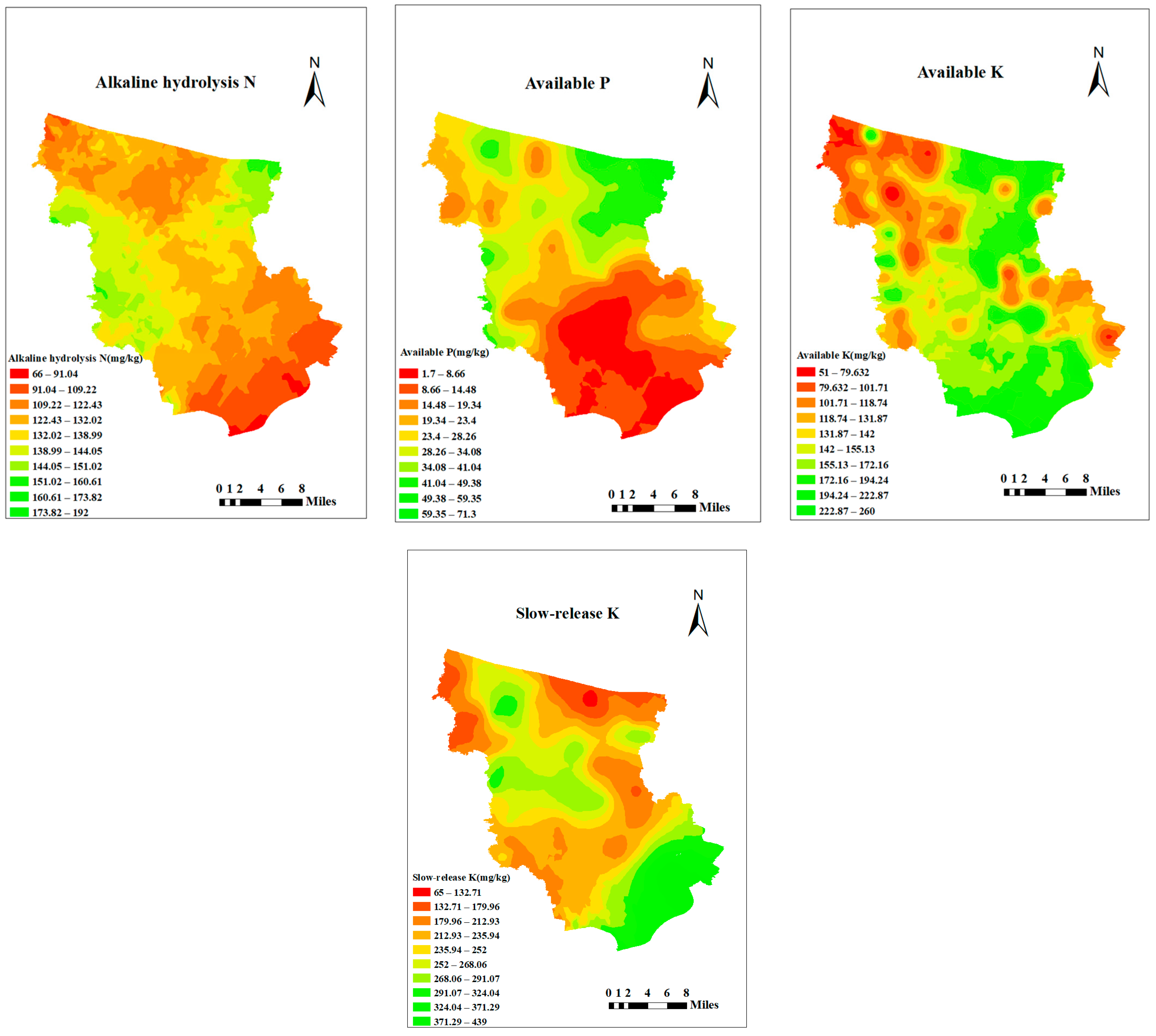
3.2.2. Soil Nutrient Spatial Distribution Status

Having determined the most suitable semivariogram function model along with its parameters, we utilized the Kriging interpolation method to draft a spatial distribution map of soil nutrients within Fengtai County, as depicted in Figure 5. Surveying all seven indicators of soil nutrient content, it becomes apparent that Fengtai County exhibits a marked spatial differentiation in its soil nutrients. Some areas prominently showcase a block-like distribution, emphasizing the spatial variability within the county. Specifically, for soil pH, the northwest regions have an acidic disposition, the central regions lean towards being acidic, and the southeastern zones generally tend towards alkalinity. Organic matter, total nitrogen, and alkali-hydrolyzable nitrogen have largely synchronous distribution patterns. Nutrient-rich sectors are predominantly in the central–western zones, whereas the northeastern areas are nutrient-scarce. We also observe sporadic pockets of lower values across the study landscape. Areas with high concentrations of available phosphorus are sporadically situated in the central–northeast zone, with some traces on the western boundary. In contrast, the southern regions predominantly showcase low-value zones. The distribution of rapid-acting potassium is notably fragmented over limited stretches. The northwest and southeast harbor the low-concentration zones, while the high-concentration areas are primarily interspersed in the northeast and southwest. A general trend can be seen where the slow-acting potassium content rises from the northern to the southern regions. However, an unmistakable high-value triangular zone dominates the central area, with a conspicuous low-value tract stretching from the southwest to the northeast.

3.3. Spatial Variability of Soil Nutrients

3.3.1. Geostatistical Analysis of Soil Nutrients

The semi-variogram parameters for the soil nutrient fitting model in Fengtai County are detailed in Table 4. The nugget value, C0, represents the variability arising from random factors. In contrast, the sill value (C0 + C) captures the impact of structural factors on the indices. The ratio C0/(C0 + C), termed the nugget-to-sill ratio, quantifies the relative contribution of random variability to the total variability [30]. A nugget-to-sill ratio in the range of 0–25% indicates a strong spatial correlation, signifying the minimal influence of randomness on the index. When the ratio lies between 25 and 75%, it reflects a moderate spatial correlation, suggesting that both random and structural factors contribute to the index’s variability. Conversely, a ratio spanning 75–100% denotes a weak spatial correlation, with the index predominantly being influenced by randomness [31]. Analysis reveals that the available potassium in Fengtai County’s soil has a moderate spatial autocorrelation. This underscores that its spatial variability stems from both structural elements, such as parent material and topography, and random influences like human activities and agricultural methods. On the other hand, other nutrient indices like pH, organic matter, Total N, alkali-hydrolyzed N, Olsen-P, and slowly released K mainly exhibit weak spatial autocorrelations, implying their variations are primarily driven by random factors. The range, which signifies the spatial correlation scale, delineates the span of spatial variability of the variables under study. For the seven nutrient indices, the spatial correlation scales, in decreasing order, are alkali-hydrolyzed N > Olsen-P > organic matter > total N > slowly released K > available K > pH. Their respective scales are 777 m, 756 m, 462 m, 415 m, 237 m, 199 m, and 165 m. Notably, alkali-hydrolyzed N exhibits the broadest range, signifying a weaker spatial autocorrelation within its 777 m radius. In contrast, pH has the most confined range, indicating that local environmental factors predominantly drive its spatial variability on a more restricted scale.

3.3.2. Spatial Autocorrelation Analysis of Soil Nutrients

The global Moran’s I index is adept at gauging the overall convergence intensity of regional variables. The strength of spatial autocorrelation can be inferred from its absolute value (refer to Table 4). Our findings highlight that every soil nutrient in Fengtai County exhibits a strong and significant spatial positive correlation (Moran’s I > 0, P < 0.01, Z > 2.58). Ranked by their global Moran’s I values, the nutrients are as follows: Olsen-P > alkali-hydrolyzed nitrogen > pH > total N > slowly released K > organic matter > available K. The most pronounced spatial clustering is reflected by the global Moran’s I value of 0.884 for available phosphorus. In contrast, quickly available potassium and organic matter, having relatively low global Moran’s I indices, show a more dispersed spatial distribution.

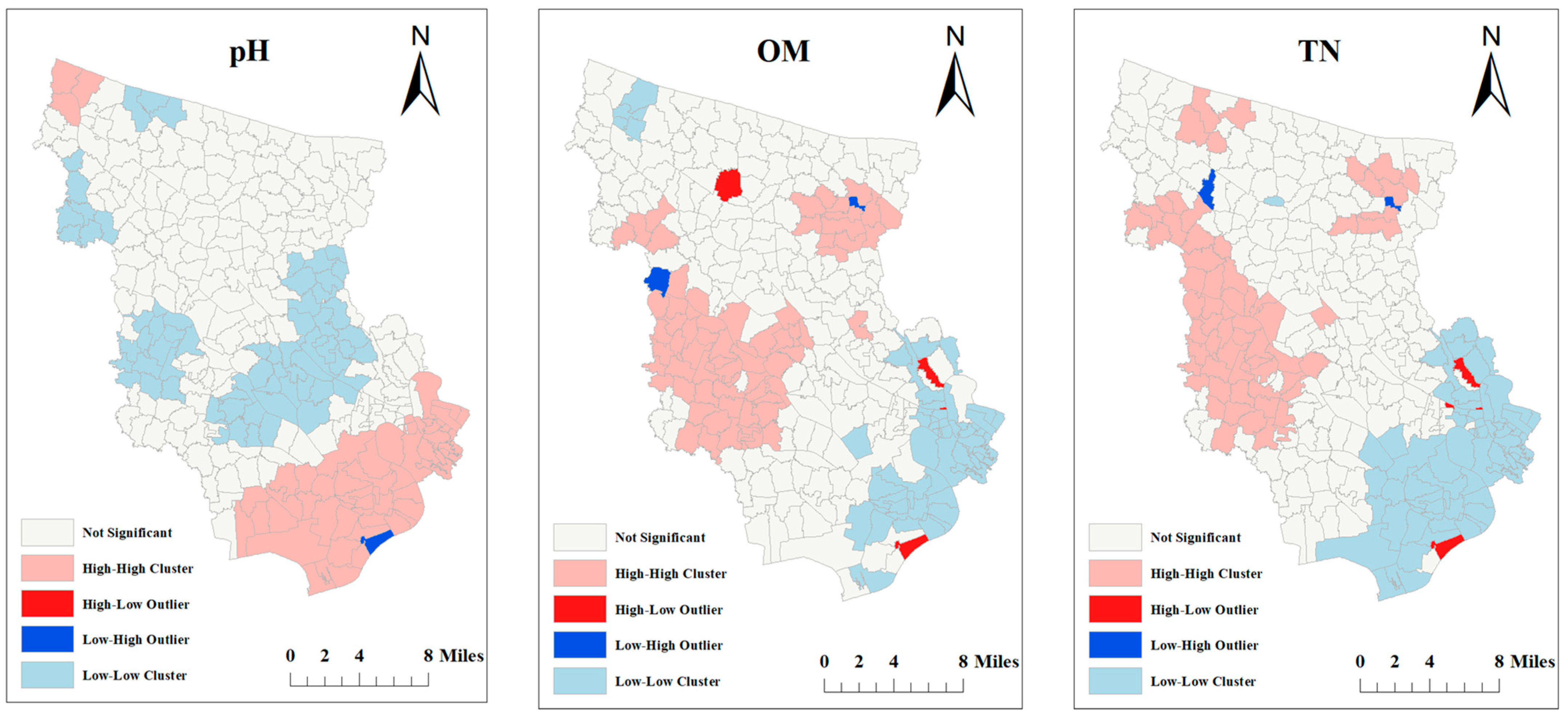
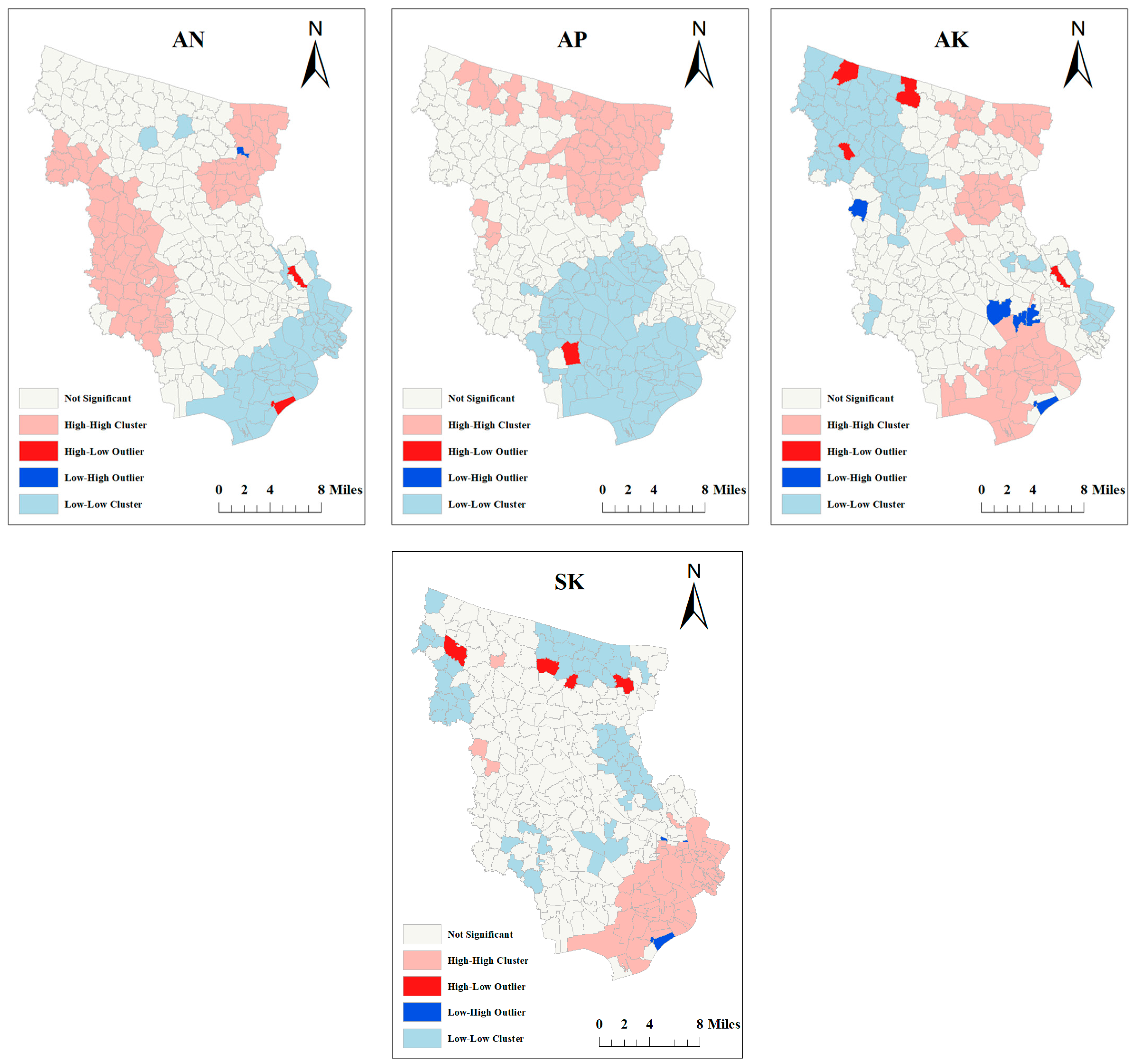
3.3.3. Spatial Clustering Analysis of Soil Nutrients

By considering each administrative village in Fengtai County as an evaluation unit, the average Kriging interpolation results within these villages were incorporated. The local Moran’s I index was subsequently determined, culminating in the LISA clustering map depicted in Figure 6. The insights gleaned from the analysis are as follows: High pH values predominantly surface in the southern regions, punctuated by pockets of low-high anomalies and a sparse presence in the northwest. Low pH values are largely centralized, with occasional appearances in the northwest. The spatial patterns of organic matter, total nitrogen, and alkali-hydrolyzed nitrogen are roughly analogous. They are largely scattered. Regions with lower values for these nutrients are chiefly situated in the southeast and sparingly in the north. Areas with higher concentrations appear in fragmented patches, primarily in the central–west and northeast regions. Both the low-high and high-low anomaly zones are interspersed within these clusters. Available phosphorus showcases distinct spatial clustering. Its low-value regions are centered in the south–central areas, accompanied by minute high-low anomaly patches. In contrast, the high-value territories are dominant in the northeast with minor representations in the central–west region. Quickly available potassium displays a patchy spatial layout for both its high and low-value clusters. The zones with lower values are mainly positioned in the northwest, occasionally in the central–west and east regions. High-value pockets are dispersed across the north, central, and southern parts, encircled by sporadic anomaly regions. The low-value clustering of slowly released potassium is broken up, emerging in the northeast, northwest, and central regions, with infrequent high-low anomaly zones. Its high-value concentrations are predominantly in the south and sparingly in the central–west region.

3.4. Assessment of Soil Fertility Status

3.4.1. Selection of Soil Indicators for the Minimum Data Set

Pearson correlation and principal component analysis (PCA) can be used to avoid data redundancy as much as possible and retain its soil interpretation information. Through principal component analysis, the eigenvalue, variance and cumulative variance contribution rate of each principal component and the common factor variance of each index are obtained (Table 5). According to the principle of eigenvalue ≥ 1, the cumulative variance contribution rate of the five principal components was 78.07%.
From Table 5, it can be seen that the index with the largest load value in the first principal component is total nitrogen content, and the index in the range of 10% is organic matter content and alkali-hydrolyzed nitrogen. Both of these two indexes have a high correlation with wheat biomass (R = 0.57, 0.57, p < 0.01), so total nitrogen, organic matter and alkali-hydrolyzed nitrogen are selected into MDS. In the second principal component, only available potassium content was a high factor load index, so available potassium was selected for MDS. In addition, available phosphorus was also significantly positively correlated with wheat biomass (R = 0.56, p < 0.05). Considering that soil-available phosphorus is closely related to crop growth and is an inherent property of soil, reflecting the nutrient supply capacity of soil to plants, soil-available phosphorus was selected into MDS. In summary, five indicators of total nitrogen, organic matter, alkali-hydrolyzable nitrogen, available phosphorus and available potassium were finally selected into MDS for SQI calculation. In addition, in order to better reflect the impact of various soil nutrient indicators on wheat biomass, we used Pearson correlation analysis to further explain it, as shown in Figure 7.

3.4.2. Indicator Scores and Weights

A linear scoring method was used to convert the soil indicators of the minimum data set into scores. The score weights of the selected indicators are shown in Figure 8 below. Finally, the SQI is calculated by adding the standardized indicator values and their weighted products to the minimum data set. The formula of SQI is as follows:
SQI = SOM × 0.225 + TN × 0.240 + AN × 0.244 + AP × 0.078 + AK × 0.2112
The soil comprehensive fertility quality index (SQI) in the study area was evaluated by principal component analysis combined with the correlation between wheat yield and soil nutrients. The results are shown in Figure 9. In this study, the selected indexes mainly included ANsoil, APsoil, AKsoil, OMsoil and TNsoil. The high-value areas of soil quality index (SQI) were concentrated in the middle and northeast of the study area, while the southeast and northwest regions were at a low level, which indicated that the soil nutrient limiting factors in the southeast and northwest regions of the study area were mainly organic matter, total nitrogen, available nitrogen, available phosphorus and available potassium. This also further cross-validated the lack of these nutrient indicators in the region, leading to the conclusion that wheat yield decreased.

4. Discussion

4.1. Characterization of Nutrient Variation and Recommendations for Zoning Management

In our research, we utilized geostatistics, merging the techniques of GS+ and GIS to tailor-fit various models. From these, the interpolation model was chosen based on each model’s optimal parameters, aiming to augment interpolation precision. Through collecting and assessing soil samples, we determined the concentrations of diverse nutrient indicators. We then employed the geostatistics analysis module for a spatial variation evaluation, defining its spatial autocorrelation and significance via the global Moran’s I index. As a result, we generated illustrative maps of soil nutrient distribution and LISA clustering. These maps shed light on the inherent relationships and spatial variation attributes of distinct soil nutrients within the study domain. The mature wheat was collected on the quadrats at the sampling points in the next year, and the correlation between its yield and each nutrient index was calculated. Principal component analysis (PCA) was used to determine the minimum data set (MDS) of soil nutrient evaluation, and the soil quality index (SQI) was calculated by linear scoring method to explore the key factors restricting soil quality in the region.
For Fengtai County, the span of soil pH is 165 m with a coefficient of variation standing at 8.22%. This, in comparison to other nutrient metrics, is the lowest. The nugget-to-sill ratio for soil pH rests at 92.6%. Drawing from these statistics, we deduce that the area’s soil pH is predominantly shaped by stochastic elements like human interventions. There’s a pronounced lack of spatial continuity, with weak spatial autocorrelation over limited extents. This causes the soil pH to manifest in a patchy, clustered distribution. On a broader note, the central sector of the surveyed region has predominantly acidic soil. Conversely, the soils in the northern and southern segments lean towards being neutral or alkaline. This spatial pH differentiation may have significant ties to the distribution of soil organic matter [32]. Soil organic matter is a pivotal determinant in steering the spatial dispersion of pH values [33]. Within the components of organic matter, the content of humic acid stands out as a crucial pointer for soil pH; notably, humic acid has the propensity to reduce soil pH [34]. Over-reliance on nitrogenous fertilizers can acidify the terrain, bringing about a pH drop [35]. Hence, for the acidic terrains in the central low-value cluster, it is prudent to embrace judicious fertilization strategies [36] and fitting cropping patterns. Incorporating an optimal quantity of substances like biochar or limestone can also serve to modulate soil pH [37], ushering in enhanced amelioration effects.
In Fengtai County, the soil demonstrates a pronounced correlation between organic matter, total nitrogen, and alkali-hydrolyzable nitrogen, with their spatial distribution patterns being notably alike. Their respective nugget ratios stand at 89.1%, 98.8%, and 99.8%. When compared to other indicators, their range of variabilities is relatively vast with values of 462 m, 415 m, and 777 m. The global Moran’s I index values for these elements are notably high, listed as 0.682, 0.783, and 0.876. This indicates that across a broad spectrum, their spatial differences are predominantly affected by random determinants, like human activities or fertilization methods. Their distribution appears concentrated, forming a patch-like appearance on nutrient maps. This may be attributed to organic matter and total nitrogen content being related to the distribution of nitrogen fertilizer [38]. The diverse agricultural practices among farmers result in the uneven distribution of these elements within the county. Notably, the variation coefficients for these factors are smaller when juxtaposed against other indicators, with values of 21.04%, 20.53%, and 19.45%. This suggests a lower general dispersal and a shift from fragmentation to uniformity in their dispersion. Both total nitrogen and organic matter critically impact crop yields [39]. Their concentrations are intrinsically linked to land use approaches, soil classifications, and the introduction of organic fertilizers [40,41]. In regions with diminished levels of organic matter, total nitrogen, and alkali-hydrolyzable nitrogen, adopting practices like straw return [42], deep tilling [43], organic crop rotation [44], and intercropping [45] can markedly elevate the soil’s organic matter and nitrogen content.
In Fengtai County, the soil’s available phosphorus block ratio stands at 85.6% over a range of 756 m. This infers that the spatial fluctuations of available phosphorus across extensive areas predominantly stem from unpredictable elements like human actions and fertilization techniques. Both its global Moran’s I index of 0.884 and coefficient of variation at 59.12% surpass other nutrient benchmarks considerably. Its spatial autocorrelation is also statistically significant (Z > 2.58), suggesting a robust aggregation trend for available phosphorus. The LISA clustering diagram reveals noticeable clusters of high and low values of available phosphorus. The northeastern sector showcases a dense high-value cluster, while the central–southern zone predominantly displays lower values. This might be due to intensified urbanization in the east, where human actions are more condensed, resulting in available phosphorus accumulation. For northeastern sectors with abundant available phosphorus, field checks are imperative to identify the cause of its heightened levels. Proactive, scientifically backed measures are crucial to avert potential agricultural runoff pollution. Conversely, in the central–southern regions with diminished phosphorus, it is advisable to employ methodical fertilization strategies, like applying foliar phosphorus [46], integrating organic fertilizers with phosphorus supplements [47], and leveraging traditional zinc fertilizers to bolster soil phosphorus efficiency [46].
As for Fengtai County’s soil-available potassium, its block ratio is 71.8% spanning a range of 199 m. This highlights that small-scale spatial fluctuations of available potassium are shaped by both unpredictable aspects, such as human interactions, and structural components like the formation of the parent material. Its global Moran’s I index sits at 0.562, indicating a more decentralized spatial distribution than other nutrient metrics. This could be attributed to individual farmer practices, which disrupt uniform tilling and fertilization approaches, leading to a patchy distribution of available potassium in certain zones. Slow-release potassium exhibits a block ratio of 97.3% across 237 m, suggesting that its minor spatial inconsistencies are mainly steered by unforeseen factors like human interventions. Its global Moran’s I index of 0.729 indicates a denser spatial spread. Using the LISA clustering diagram as a reference, regions with elevated slow-release potassium are more clustered, while low-value areas appear sporadic. This pattern might correlate with the variety of crops cultivated. As crops utilize available potassium, leading to its shortfall, the soil’s slow-release potassium transforms into available potassium to maintain a balance [48]. For zones with potassium scarcity, implementing practices like standard straw reintroduction to plots and judicious potassium fertilizer applications can notably enhance soil potassium concentration [49].

4.2. Research Innovations and Ideas for Improvement

In this research, soil nutrient spatial autocorrelation was predominantly strong, influenced chiefly by natural factors like topography, soil type, parent material, and climate, promoting a trend toward the homogenization of soil nutrient variability. Geostatistical analysis revealed that soil pH is more prone to being influenced by stochastic factors, including human activities and fertilization practices, aligning with findings from other statistical studies [50]. Similarly, the variability in soil organic matter, total nitrogen, available nitrogen, and available phosphorus was affected by random factors such as human interventions, a perspective endorsed by numerous scholars; notably, available phosphorus exhibited a coefficient of variation much higher than that of other nutrients, echoing the comparisons made by Tan [50,51] among multiple nutrients. Its Moram’s I index was also the highest, underscoring the tendency of available phosphorus to accumulate [52]. The block base ratio for total nitrogen, available nitrogen, and slow-release potassium was notably high, mirroring Jing and others’ [53] observations with total nitrogen and available nitrogen, thus highlighting their vulnerability to stochastic factors like human activities. Conversely, the block base ratio for readily available potassium was the lowest, with research indicating that soil potassium primarily originates from the weathering of parent materials [54], suggesting that readily available potassium is subject to the combined effects of structural factors such as parent material and stochastic factors like human activities. From the data perspective, although there were significant deviations in this study’s results compared to others, the overall patterns of nutrient differences remained consistent. This discrepancy could be attributed to the extensive number of sampling locations within this study area, where the spatial variability characteristics of area variables altered with the sampling point layout’s scale. When sampling scales are markedly smaller than the natural distribution scales of elements like parent material and topography, spatial variability tends to lean towards being governed by stochastic factors, such as fertilization levels from human intervention [55]. This phenomenon has also been confirmed in studies involving high-density sampling [56,57].
Our study leverages high-density, randomly sampled data from Fengtai County, applying the block base ratio and the semivariogram’s range to delineate spatial autocorrelation and its influence radius. The global Moran’s I index was employed to gauge the strength and significance of spatial autocorrelation, while the variance coefficient of nutrient statistics was juxtaposed with research outcomes. Furthermore, Kriging interpolation and the local Moran’s I index were utilized to generate maps depicting nutrient distribution and LISA cluster analysis, thereby methodically illustrating the spatial variability and interconnectedness of different soil nutrients within the study locale. Presently, the independent application of geostatistics or the Moran’s I index predominates among scholars for exploring soil nutrient spatial variability, with combined methodological approaches being relatively unexplored. This thorough examination of soil nutrients in our research, coupled with a comparative analysis, aims to serve as a dependable framework for future investigations into the spatial variability of soil nutrients across various regions.

4.3. Assessment of Soil Fertility Quality Status

In this study, five soil indicators were screened by principal component analysis, and finally, organic matter, total nitrogen, available potassium and available phosphorus and nitrogen were identified as MDS. The SQI model is constructed according to the determined MDS. The cumulative contribution rate of the MDS soil index constructed in this study was 69.63%. Correlation analysis showed that all soil indexes were significantly correlated with MDS soil index construction. Soil organic matter, available potassium, available phosphorus, nitrate nitrogen and total nitrogen play an important role in the construction of soil nutrient evaluation MDS [58]. This study also found that soil total nitrogen, hydrolyzable nitrogen and total potassium accounted for a larger weight in MDS, and their contribution to SQI was also greater, indicating that these indicators were important factors for evaluating soil fertility and productivity. Different factors were selected to participate in the evaluation of soil quality, resulting in slightly different key factors for the final evaluation. Soil quality assessment is sufficient to study specific land functions and land use types.
In addition, the purpose of soil quality assessment is to determine the soil quality status by analyzing soil indicators, and then evaluate the yield potential of local wheat. Soil quality plays an important role in improving the environment and crop productivity. Although previous studies have used many methods to calculate soil quality, the relationship between SQI and crop biomass is less mentioned [59]. Therefore, their research may be lack of biological significance. In this study, there was a significant (p < 0.01) positive correlation between wheat yield and soil quality index. Wheat yield increased with the increase in soil quality, indicating that the soil properties selected from the full data set had biological significance and could effectively evaluate the status of soil as a wheat production medium. The results of Li et al. [60] showed that the main reason for the difference in plant yield was the difference in soil quality, and plant yield was the embodiment of soil quality. Duan [61] found that soil biological properties can better respond to soil quality changes, which is an important part of soil quality evaluation.
According to the distribution of the SQI index, referring to the results of previous studies [62,63], most of the soil nutrients in this study area were at a high level (0.54–0.74) or a low level (0.14–0.42). The results of Moran‘s index analysis showed that the nutrient contents were significantly different in space. The high-value areas of soil organic matter, total nitrogen, alkali-hydrolyzable nitrogen and available phosphorus were distributed in the central and northeastern parts of the study area, which was consistent with the spatial distribution of soil SQI index. The reason for the large fluctuation in soil fertility may be caused by uneven fertilization. The author’s investigation found that the central part of the study area has abundant water sources, concentrated population density, and frequent human farming activities. However, the population density in the northwest and southeast is low, and there is a lack of standardized agricultural fertilization management, that is, the input of organic fertilizer and nitrogen fertilizer is insufficient, and the application of potassium fertilizer is less. Fertilization measures should be formulated to increase the input of organic matter, nitrogen fertilizer and potassium fertilizer in the area for a long time. In land use, it is necessary to strengthen the combination of use and nutrition, standardize the return of straw to the field, improve the soil nutrient content in the southeast and northwest of the study area, and prevent serious soil degradation caused by planting.

5. Conclusions

In Fengtai County, the mean measures for soil pH, organic matter, total nitrogen, alkali-hydrolyzable nitrogen, available phosphorus, available potassium, and slow-release potassium are recorded as 6.68, 25.04 g/kg, 1.51 g/kg, 134.51 mg/kg, 26.00 mg/kg, 137.23 mg/kg, and 238.69 mg/kg, in that order. The fluctuation across these nutrients is of a moderate scale. The most suitable modeling fit for the soil pH in Fengtai is the Gaussian model. Conversely, organic matter, total nitrogen, and available potassium align more with the spherical model. The alkali-hydrolyzable nitrogen, available phosphorus, and slow-release potassium are most aptly represented by the exponential model. The spatial interconnectedness of available potassium is moderate, contrasting with the other nutrients, which exhibit a comparatively weaker spatial correlation. This infers that the spatial diversities of soil nutrients within the study’s scope are predominantly governed by human activities, fertilization practices, and other stochastic factors. All nutrient elements within Fengtai County’s soil showcase a markedly positive spatial association. The sequence of this spatial correlation unfolds as follows: available phosphorus > alkali-hydrolyzable nitrogen > pH > total nitrogen > slow-release potassium > organic matter > available potassium. Distinct nutrients within Fengtai County’s soil display different extents of spatial dispersion, each adhering to its distinctive distribution layout. In general, the northern and southern extremes of the study area lean towards lower nutrient levels, while the central part is richer in content. The north is characterized by high nutrient clusters, whereas the south predominantly displays low nutrient concentrations. Notably, the spatial agglomeration of available phosphorus is distinctly evident, with pronounced high-value clusters in the northern zone and clear low-value clusters in the southern segment.
The spatial distribution of soil fertility quality in Fengtai County is quite different. The uneven distribution of population and scattered fertilization are the main reasons for the fluctuation of fertility. Organic matter, total nitrogen, alkali-hydrolyzed nitrogen and available potassium are the limiting factors of soil nutrients in the study area. In the future, in order to ensure the soil nutrient accumulation and sustainable development of agriculture in the rice–wheat rotation area of Fengtai County, it is suggested to formulate standardized precise fertilization measures. For the areas with poor soil fertility in the southeast and northwest of the study area, it is necessary to further study and determine the optimal ratio of nitrogen, phosphorus and potassium fertilizers while increasing fertilization.

Author Contributions

Data Curation: Z.J. and Z.Y.; Formal Analysis: M.H., D.C. and Z.J.; Funding Acquisition: Z.J.; Investigation: Z.J., T.W., Y.Z. (Yupeng Zhang), M.Z. and W.W.; Methodology: Z.J., X.L. and Y.Z. (Yuzhi Zhou); Writing—Original Draft: Z.J. and Y.Z. (Yuzhi Zhou); Writing—Review and Editing: Z.J. and Y.Z. (Yuzhi Zhou). All authors have read and agreed to the published version of the manuscript.

Funding

The authors are grateful for the financial support provided by Key research and development plan of Anhui Province (No. S202104a06020064), The China Geological Survey (Comprehensive Survey of Natural Resources in the Middle Reaches of the Yellow River (Shaanxi Section), Grant Nos. DD20220868), the Opening Foundation of Anhui Province Engineering Laboratory for Mine Ecological Remediation (No. KS-2022-002), the Opening Foundation of Anhui Green Mine Engineering Research and Development Center in 2022, the Opening Foundation of Anhui Province Engineering Laboratory of Water and Soil Resources Comprehensive Utilization and Ecological Protection in High Groundwater Mining Area (No. 2022-WSREPMA-05). The authors express their sincere thanks and gratitude to the anonymous reviewers due to their positive comments and constructive suggestions.

Data Availability Statement

The original contributions presented in the study are included in the article, further inquiries can be directed to the corresponding author.

Conflicts of Interest

The authors declare no conflict of interest.

References

  1. Haq, S.M.; Hassan, M.; Jan, H.A.; Al-Ghamdi, A.A.; Ahmad, K.; Abbasi, A.M. Traditions for future cross-national food security—Food and foraging practices among different native communities in the Western Himalayas. Biology 2022, 11, 455. [Google Scholar] [CrossRef] [PubMed]
  2. Bogunovic, I.; Trevisani, S.; Seput, M.; Juzbasic, D.; Durdevic, B. Short-range and regional spatial variability of soil chemical properties in an agro-ecosystem in eastern Croatia. Catena 2017, 154, 50–62. [Google Scholar] [CrossRef]
  3. Rinot, O.; Levy, G.J.; Steinberger, Y.; Svoray, T.; Eshel, G. Soil health assessment: A critical review of current methodologies and a proposed new approach. Sci. Total Environ. 2019, 648, 1484–1491. [Google Scholar] [CrossRef] [PubMed]
  4. Socher, S.A.; Prati, D.; Boch, S.; Müller, J.; Klaus, V.H.; Hölzel, N.; Fischer, M. Direct and productivity-mediated indirect effects of fertilization, mowing and grazing on grassland species richness. J. Ecol. 2012, 100, 1391–1399. [Google Scholar] [CrossRef]
  5. Jiang, Z.; Zhou, Y.; Chen, D. Effects of microbial fungicide and soybean straw biochar on nutrients and quality of Brassica napus in black soil of sand ginger. China Melon Veg. 2024, 37, 133–139. [Google Scholar] [CrossRef]
  6. Waring, B.G.; Álvarez-Cansino, L.; Barry, K.E.; Becklund, K.K.; Dale, S.; Gei, M.G.; Keller, A.B.; Lopez, O.R.; Markesteijn, L.; Mangan, S.; et al. Pervasive and strong effects of plants on soil chemistry: A meta-analysis of individual plant ‘Zinke’ effects. Proc. R. Soc. B Biol. Sci. 2015, 282, 20151001. [Google Scholar] [CrossRef] [PubMed]
  7. Long, L.; Liu, Y.; Chen, X.; Guo, J.; Li, X.; Guo, Y.; Zhang, X.; Lei, S. Analysis of spatial variability and influencing factors of soil nutrients in western China: A Case Study of the Daliuta Mining Area. Sustainability 2022, 14, 2793. [Google Scholar] [CrossRef]
  8. Samuel, A.D.; Bungau, S.; Tit, D.M.; Melinte, C.E.; Purza, L.; Badea, G.E. Effects of long term application of organic and mineral fertilizers on soil enzymes. Rev. Chim. 2018, 69, 2608–2612. [Google Scholar] [CrossRef]
  9. Florinsky, I.V.; Eilers, R.G.; Lelyk, G.W. Prediction of soil salinity risk by digital terrain modeling in the Canadian prairies. Can. J. Soil Sci. 2000, 80, 455–463. [Google Scholar] [CrossRef]
  10. Kral, F.; Corstanje, R.; White, J.R.; Veronesi, F. A geostatistical analysis of soil properties in the Davis Pond Mississippi freshwater diversion. Soil Sci. Soc. Am. J. 2012, 76, 1107–1118. [Google Scholar] [CrossRef]
  11. Fu, W.; Dong, J.; Ding, L.; Yang, H.; Ye, Z.; Zhao, K. Spatial correlation of nutrients in a typical soil-hickory system of southeastern China and its implication for site-specific fertilizer application. Soil Tillage Res. 2022, 217, 105265. [Google Scholar] [CrossRef]
  12. Thakur, N.; Sharma, R.; Kumar, A.; Sood, K. Soil fertility appraisal for pea growing regions of Himachal Pradesh using GPS and GIS techniques. Indian J. Agric. Res. 2021, 55, 452–457. [Google Scholar] [CrossRef]
  13. Liu, Y.; Chen, Y.; Wu, Z.; Wang, B.; Wang, S. Geographical detector-based stratified regression kriging strategy for mapping soil organic carbon with high spatial heterogeneity. Catena 2021, 196, 104953. [Google Scholar] [CrossRef]
  14. Mishra, U.; Hugelius, G.; Shelef, E.; Yang, Y.; Strauss, J.; Lupachev, A.; Harden, J.W.; Jastrow, J.D.; Ping, C.L.; Riley, W.J.; et al. Spatial heterogeneity and environmental predictors of permafrost region soil organic carbon stocks. Sci. Adv. 2021, 7, eaaz5236. [Google Scholar] [CrossRef]
  15. Chen, S.; Lin, B.; Li, Y.; Zhou, S. Spatial and temporal changes of soil properties and soil fertility evaluation in a large grain-production area of subtropical plain, China. Geoderma 2020, 357, 113937. [Google Scholar] [CrossRef]
  16. Wang, R.; Zou, R.; Liu, J.; Liu, L.; Hu, Y. Spatial distribution of soil nutrients in farmland in a hilly region of the pearl river delta in China based on geostatistics and the inverse distance weighting method. Agriculture 2021, 11, 50. [Google Scholar] [CrossRef]
  17. Yan, P.; Peng, H.; Yan, L.; Zhang, S.; Chen, A.; Lin, K. Spatial variability in soil pH and land use as the main influential factor in the red beds of the Nanxiong Basin, China. PeerJ 2019, 7, e6342. [Google Scholar] [CrossRef] [PubMed]
  18. Lu, R.K. Methods of Analysis of Soil and Agro-Chemistry; China Agricultural Science and Technology Press: Beijing, China, 2000. [Google Scholar]
  19. Dai, W.; Zhao, K.; Fu, W.; Jiang, P.; Li, Y.; Zhang, C.; Gielen, G.; Gong, X.; Li, Y.; Wang, H.; et al. Spatial variation of organic carbon density in topsoils of a typical subtropical forest, southeastern China. Catena 2018, 167, 181–189. [Google Scholar] [CrossRef]
  20. Fu, W.; Zhao, K.; Jiang, P.; Ye, Z.; Tunney, H.; Zhang, C. Field-scale variability of soil test phosphorus and other nutrients in grasslands under long-term agricultural managements. Soil Res. 2013, 51, 503–512. [Google Scholar] [CrossRef]
  21. Ju, Q.; Hu, Y.; Xie, Z.; Liu, Q.; Zhang, Z.; Liu, Y.; Peng, T.; Hu, T. Characterizing spatial dependence of boron, arsenic, and other trace elements for Permian groundwater in Northern Anhui plain coal mining area, China, using spatial autocorrelation index and geostatistics. Environ. Sci. Pollut. Res. 2023, 30, 39184–39198. [Google Scholar] [CrossRef]
  22. Shen, Y.; Li, J.; Chen, F.; Cheng, R.; Xiao, W.; Wu, L.; Zeng, L. Correlations between forest soil quality and aboveground vegetation characteristics in Hunan Province, China. Front. Plant Sci. 2022, 13, 1009109. [Google Scholar] [CrossRef]
  23. Raiesi, F. A minimum data set and soil quality index to quantify the effect of land use conversion on soil quality and degradation in native rangelands of upland arid and semiarid regions. Ecol. Indic. 2017, 75, 307–320. [Google Scholar] [CrossRef]
  24. Yu, P.; Han, D.; Liu, S.; Wen, X.; Huang, Y.; Jia, H. Soil quality assessment under different land uses in an alpine grassland. Catena 2018, 171, 280–287. [Google Scholar] [CrossRef]
  25. Andrews, S.S.; Karlen, D.L.; Mitchell, J.P. A comparison of soil quality indexing methods for vegetable production systems in Northern California. Agric. Ecosyst. Environ. 2002, 90, 25–45. [Google Scholar] [CrossRef]
  26. National Soil Census Office. Soil of China; China Agricultural Press: Beijing, China, 1998. [Google Scholar]
  27. Zhang, X.Y.; Yue-Yu, S.U.; Zhang, X.D.; Kai, M.E.; Herbert, S.J. Spatial variability of nutrient properties in black soil of northeast China. Pedosphere 2007, 17, 19–29. [Google Scholar] [CrossRef]
  28. Xie, Y.; Chen, T.B.; Lei, M.; Yang, J.; Guo, Q.J.; Song, B.; Zhou, X.Y. Spatial distribution of soil heavy metal pollution estimated by different interpolation methods: Accuracy and uncertainty analysis. Chemosphere 2011, 82, 468–476. [Google Scholar] [CrossRef] [PubMed]
  29. Li, Z.J.; Meng, Y.S.; Zheng, M.L.; Wang, H.H.; Chen, F.R.; Hu, H.X.; Ma, Y.H. Spatial variability and ecological health risk assessment of heavy metals in farmland soil-rice system in a watershed of China. J. Agro-Environ. Sci. 2021, 40, 957–968. [Google Scholar]
  30. Burrough, P.A. Multiscale sources of spatial variation in soil. I. The application of fractal concepts to nested levels of soil variation. J. Soil Sci. 1983, 34, 577–597. [Google Scholar] [CrossRef]
  31. Gao, Z.; Fu, W.; Zhang, M.; Zhao, K.; Tunney, H.; Guan, Y. Potentially hazardous metals contamination in soil-rice system and it’s spatial variation in Shengzhou City, China. J. Geochem. Explor. 2016, 167, 62–69. [Google Scholar] [CrossRef]
  32. Ou, Y.; Rousseau, A.N.; Wang, L.; Yan, B. Spatio-temporal patterns of soil organic carbon and pH in relation to environmental factors—A case study of the Black Soil Region of Northeastern China. Agric. Ecosyst. Environ. 2017, 245, 22–31. [Google Scholar] [CrossRef]
  33. Mao, W.; Li, W.; Gao, H. pH variation and the driving factors of farmlands in Yangzhou for 30 years. J. Plant Nutr. Fertil. 2017, 23, 883. [Google Scholar]
  34. Angelova, V.R.; Akova, V.I.; Artinova, N.S.; Ivanov, K.I. The effect of organic amendments on soil chemical characteristics. Bulg. J. Agric. Sci. 2013, 19, 958–971. [Google Scholar]
  35. Bogunovic, I.; Mesic, M.; Zgorelec, Z.; Jurisic, A.; Bilandzija, D. Spatial variation of soil nutrients on sandy-loam soil. Soil Tillage Res. 2014, 144, 174–183. [Google Scholar] [CrossRef]
  36. Ning, Q.; Chen, L.; Jia, Z.; Zhang, C.; Ma, D.; Li, F.; Zhang, J.; Li, D.; Han, X.; Cai, Z.; et al. Multiple long-term observations reveal a strategy for soil pH-dependent fertilization and fungal communities in support of agricultural production. Agric. Ecosyst. Environ. 2020, 293, 106837. [Google Scholar] [CrossRef]
  37. Dai, Z.; Zhang, X.; Tang, C.; Muhammad, N.; Wu, J.; Brookes, P.C.; Xu, J. Potential role of biochars in decreasing soil acidification-a critical review. Sci. Total Environ. 2017, 581, 601–611. [Google Scholar] [CrossRef]
  38. Li, J.; Jian, S.; Lane, C.S.; Guo, C.; Lu, Y.; Deng, Q.; Mayes, M.A.; Dzantor, K.E.; Hui, D. Nitrogen fertilization restructured spatial patterns of soil organic carbon and total nitrogen in switchgrass and gamagrass croplands in Tennessee USA. Sci. Rep. 2020, 10, 1211. [Google Scholar] [CrossRef]
  39. Gao, P.; Wang, B.; Geng, G.; Zhang, G. Spatial distribution of soil organic carbon and total nitrogen based on GIS and geostatistics in a small watershed in a hilly area of northern China. PLoS ONE 2013, 8, e83592. [Google Scholar]
  40. Liu, D.; Wang, Z.; Zhang, B.; Song, K.; Li, X.; Li, J.; Li, F.; Duan, H. Spatial distribution of soil organic carbon and analysis of related factors in croplands of the black soil region, Northeast China. Agric. Ecosyst. Environ. 2006, 113, 73–81. [Google Scholar] [CrossRef]
  41. Wang, X.; Li, Y.; Chen, Y.; Lian, J.; Luo, Y.; Niu, Y.; Gong, X. Spatial pattern of soil organic carbon and total nitrogen, and analysis of related factors in an agro-pastoral zone in Northern China. PLoS ONE 2018, 13, e0197451. [Google Scholar] [CrossRef]
  42. Huang, T.; Yang, N.; Lu, C.; Qin, X.; Siddique, K.H. Soil organic carbon, total nitrogen, available nutrients, and yield under different straw returning methods. Soil Tillage Res. 2021, 214, 105171. [Google Scholar] [CrossRef]
  43. Alcántara, V.; Don, A.; Well, R.; Nieder, R. Deep ploughing increases agricultural soil organic matter stocks. Glob. Change Biol. 2016, 22, 2939–2956. [Google Scholar] [CrossRef] [PubMed]
  44. Gadermaier, F.; Berner, A.; Fließbach, A.; Friedel, J.K.; Mäder, P. Impact of reduced tillage on soil organic carbon and nutrient budgets under organic farming. Renew. Agric. Food Syst. 2012, 27, 68–80. [Google Scholar] [CrossRef]
  45. Lai, H.; Gao, F.; Su, H.; Zheng, P.; Li, Y.; Yao, H. Nitrogen distribution and soil microbial community characteristics in a legume–cereal intercrop** system: A review. Agronomy 2022, 12, 1900. [Google Scholar] [CrossRef]
  46. Bindraban, P.S.; Dimkpa, C.O.; Pandey, R. Exploring phosphorus fertilizers and fertilization strategies for improved human and environmental health. Biol. Fertil. Soils 2020, 56, 299–317. [Google Scholar] [CrossRef]
  47. Ma, X.; Hei, R.; Yao, Y.; Han, F.; Yang, G.; Guo, D.; Tang, M.; Luo, J.; Ma, Y. Soil fertility characteristics and strategy of fertilization for the typical grape-growing district in northern Jiangsu Province: A case study of Guannan County. J. Agric. Resour. Environ. 2023, 40, 782. [Google Scholar]
  48. Zhang, X.-Z.; Li, T.-X.; Zhou, J.-X.; Zhang, R.-S. Study on the Farmland Nutrient Balance and the Dynamic Variation Tendency of Soil Nutrients in Zitong County. Sichuan Nongye Daxue Xuebao 2004, 22, 53–57. [Google Scholar] [CrossRef]
  49. Dong, W.; Zhang, X.; Wang, H. Effect of different fertilizer application on the soil fertility of paddy soils in red soil region of southern China. PLoS ONE 2012, 7, e44504. [Google Scholar] [CrossRef]
  50. Dang, C.; Kong, F.; Li, Y.; Jiang, Z.; Xi, M. Soil inorganic carbon dynamic change mediated by anthropogenic activities: An integrated study using meta-analysis and random forest model. Sci. Total Environ. 2022, 835, 155463. [Google Scholar] [CrossRef]
  51. Moore, I.D.; Gessler, P.E.; Nielsen, G.A.; Peterson, G.A. Soil attribute prediction using terrain analysis. Soil Sci. Soc. Am. J. 1993, 57, 443–452. [Google Scholar] [CrossRef]
  52. Hou, E.; Wen, D.; Jiang, L.; Luo, X.; Kuang, Y.; Lu, X.; Chen, C.; Allen, K.T.; He, X.; Huang, X.; et al. Latitudinal patterns of terrestrial phosphorus limitation over the globe. Ecol. Lett. 2021, 24, 1420–1431. [Google Scholar] [CrossRef]
  53. Jiang, N.W.; Tong, G.P.; Ye, Z.Q. Spatial variability of soil fertility properties and its affecting factors of Qingliangfeng Nature Reserve, Zhejiang. Acta Ecol. Sin. 2022, 42, 2430–2441. [Google Scholar] [CrossRef]
  54. Zörb, C.; Senbayram, M.; Peiter, E. Potassium in agriculture–status and perspectives. J. Plant Physiol. 2014, 171, 656–669. [Google Scholar] [CrossRef]
  55. Liu, Y.; Lv, J.; Zhang, B.; Bi, J. Spatial multi-scale variability of soil nutrients in relation to environmental factors in a typical agricultural region, Eastern China. Sci. Total Environ. 2013, 450, 108–119. [Google Scholar] [CrossRef]
  56. Mazzarino, M.J.; Bertiller, M.B.; Sain, C.; Satti, P.; Coronato, F. Soil nitrogen dynamics in northeastern Patagonia steppe under different precipitation regimes. Plant Soil 1998, 202, 125–131. [Google Scholar] [CrossRef]
  57. Tang, X.; Xia, M.; Guan, F.; Fan, S. Spatial distribution of soil nitrogen, phosphorus and potassium stocks in Moso bamboo forests in subtropical China. Forests 2016, 7, 267. [Google Scholar] [CrossRef]
  58. Li, H.; Zhu, N.; Wang, S.; Gao, M.; Xia, L.; Kerr, P.G.; Wu, Y. Dual benefits of long-term ecological agricultural engineering: Mitigation of nutrient losses and improvement of soil quality. Sci. Total Environ. 2020, 721, 137848. [Google Scholar] [CrossRef] [PubMed]
  59. Qiu, X.; Peng, D.; Wang, H.; Wang, Z.; Cheng, S. Minimum data set for evaluation of stand density effects on soil quality in Larix principis-rupprechtii plantations in North China. Ecol. Indic. 2019, 103, 236–247. [Google Scholar] [CrossRef]
  60. Li, P.; Zhang, T.; Wang, X.; Yu, D. Development of biological soil quality indicator system for subtropical China. Soil Tillage Res. 2013, 126, 112–118. [Google Scholar] [CrossRef]
  61. Duan, C.; Li, J.; Zhang, B.; Wu, S.; Fan, J.; Feng, H.; He, J.; Siddique, K.H. Effect of bio-organic fertilizer derived from agricultural waste resources on soil properties and winter wheat (Triticum aestivum L.) yield in semi-humid drought-prone regions. Agric. Water Manag. 2023, 289, 108539. [Google Scholar] [CrossRef]
  62. Xing, Y.; Wang, N.; Niu, X.; Jiang, W.; Wang, X. Assessment of potato farmland soil nutrient based on MDS-SQI Model in the Loess Plateau. Sustainability 2021, 13, 3957. [Google Scholar] [CrossRef]
  63. Mamehpour, N.; Rezapour, S.; Ghaemian, N. Quantitative assessment of soil quality indices for urban croplands in a calcareous semi-arid ecosystem. Geoderma 2021, 382, 114781. [Google Scholar] [CrossRef]
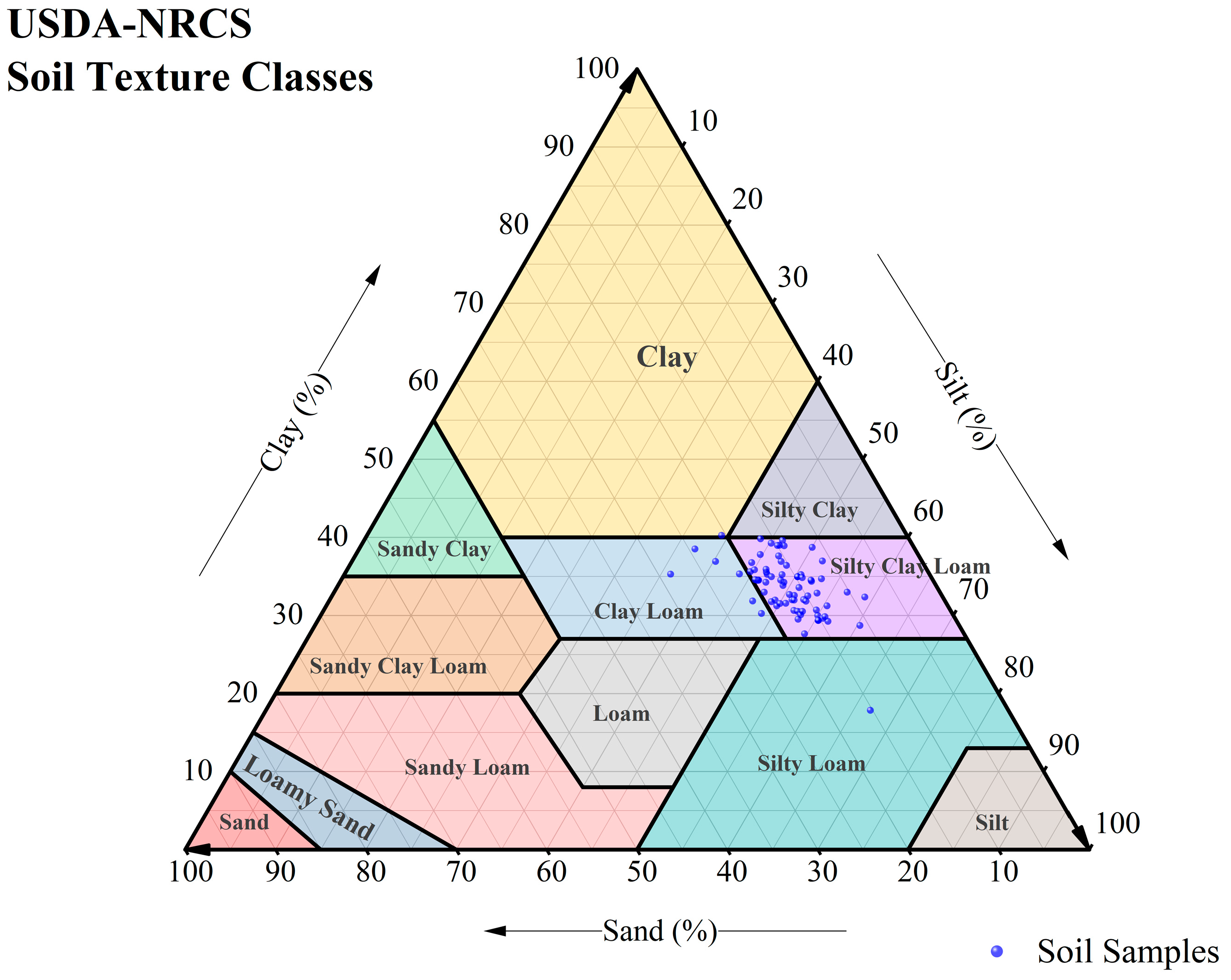
Figure 1. Textural distribution of typical sampling sites in the study area.
Applsci 14 09087 g001
Figure 2. The study area and soil sampling site. Note: The green area in the map of China is the province where the study area is located, and the red area on the right side is the study area.
Applsci 14 09087 g002
Figure 3. DEM elevation map of the study area.
Applsci 14 09087 g003
Figure 4. Map of land use types in the study area.
Applsci 14 09087 g004
Figure 5. Spatial distribution of various soil nutrients in Fengtai County.
Applsci 14 09087 g005aApplsci 14 09087 g005b
Figure 6. LISA cluster distribution of soil nutrients in Fengtai County.
Applsci 14 09087 g006aApplsci 14 09087 g006b
Figure 7. Heat map of correlation between wheat biomass and soil nutrients.
Applsci 14 09087 g007
Figure 8. Indicator weight values for each dataset of soil quality evaluation.
Applsci 14 09087 g008
Figure 9. Distribution of soil quality index (SQI) levels in the study area.
Applsci 14 09087 g009
Table 1. Physical properties of soils in the study area.
LevelDepth
(cm)
Sand
(%)
Silt
(%)
Clay
(%)
Bulk Density (g/cm3)Porosity
(%)
A0–1516.58 ± 0.53 a33.61 ± 0.66 a49.82 ± 1.53 d1.32 ± 0.012 b41.46 ± 0.08 c
B115–3019.03 ± 0.51 b34.65 ± 0.71 b46.32 ± 1.52 a1.34 ± 0.009 bc39.25 ± 0.07 a
B230–5316.90 ± 0.55 a35.58 ± 0.63 c47.52 ± 1.47 b1.31 ± 0.011 a41.17 ± 0.08 bc
C53–10016.59 ± 0.41 a34.87 ± 1.07 b48.54 ± 1.43 c1.35 ± 0.010 c40.62 ± 0.09 b
Note: Layer A is the surface layer of soil, layer B is the middle layer of soil, and layer C is the deep layer of soil. The data is the average value. The different lowercase letters a–d after the same column value indicate that there is a significant difference between different treatment groups (p < 0.05 ), the same below.
Table 2. Descriptive statistical characteristics of soil nutrients in the study area.
IndexMinMaxMeanStandard DeviationMedianCV/%Distribution
Pattern
SkewnessKurtosis
pH5.038.206.680.556.728.22%Normal Distributions0.103.71
Organic matter7.4040.1325.045.2725.5421.04%Normal Distributions−0.534.19
Total N0.682.961.510.311.5620.53%Normal Distributions0.446.79
Alkalihydrolyzed Nitrogen66.07192.73129.8825.26134.5119.45%Normal Distributions−0.392.77
Olsen-P1.7071.3128.9617.1226.0059.12%Log-normal distribution0.432.39
Available K51.13260.45141.9449.11137.2334.59%Log-normal distribution0.372.21
Slowly released K65.04439.27238.3371.75238.6930.11%Log-normal distribution0.363.30
Table 3. Prediction errors of different fitted models for soil nutrients in Fengtai County.
IndexModelPrediction Errors
MeanRoot Mean SquareStandardized MeanRoot Mean Square StandardizedAverage Standard Error
pHSpherical−0.014860.49547−0.022311.075780.45501
Exponential −0.016600.49438−0.026871.061230.46129
Gaussian−0.013980.49290−0.021021.061550.45639
Organic matterSpherical0.034035.524340.007311.046845.24727
Exponential0.044025.499410.008061.039335.26406
Gaussian0.040735.531590.008021.047815.24555
Total NSpherical0.004160.318910.013521.015810.31135
Exponential0.004680.313630.014060.995180.31136
Gaussian0.004830.314290.014640.997210.31344
Alkali-hydrolyzed NitrogenSpherical0.4316125.983510.015410.9952526.1469
Exponential0.4203226.097320.015150.9979526.17411
Gaussian0.4208726.075510.015170.9977826.16108
Olsen-PSpherical−0.0103115.342830.000751.0275714.84871
Exponential−0.0186015.373510.000371.0321514.83651
Gaussian−0.0699915.39364−0.003121.0301614.86627
Available KSpherical0.0031545.635730.003310.9997245.06263
Exponential0.6108046.353050.013521.0157945.35491
Gaussian−0.0271745.927180.003091.0282344.09285
Slowly released KSpherical−0.0986957.649190.000931.0037957.30993
Exponential0.0880856.985180.002980.9807857.87014
Gaussian−0.6030357.67448−0.006510.9982657.64336
Table 4. Parameters of the semivariogram for soil nutrients in Fengtai County and the global Moran’s I.
IndexModelNugget
(C0)
Still
(C0 + C)
Nugget/Still
C0/(C0 + C)
Range (km)Moran’s IStandard Z Value
pHGaussian0.2360.2550.9260.1650.87124.962
Organic matterSpherical22.8025.590.8910.4620.68219.563
Total NSpherical0.1170.1190.9880.4150.78322.464
Alkalihydrolyzed NitrogenExponential412.0412.90.9980.7770.87625.095
Olsen-PExponential266.3311.10.8560.7560.88425.353
Available KSpherical941.213110.7180.1990.56216.136
Slowly released KExponential367037720.9730.2370.72920.921
Table 5. Correlation coefficient matrix of chemical properties of soils.
IngredientpHSOMTNANAPSKAK
PC1−0.6790.9050.9340.9190.523−0.4990.188
PC20.5350.026−0.068−0.2140.1180.4770.860
Disclaimer/Publisher’s Note: The statements, opinions and data contained in all publications are solely those of the individual author(s) and contributor(s) and not of MDPI and/or the editor(s). MDPI and/or the editor(s) disclaim responsibility for any injury to people or property resulting from any ideas, methods, instructions or products referred to in the content.

