Abstract
A hydraulic jump phenomenon is exciting in turbulent flow as it causes large-scale turbulence and high-energy loss. This paper investigates the hydraulic jump characteristics of right triangular prism rough beds. The renormalization group RNG k-ε turbulent model and the volume of fluid (VOF) method in a CFD model are utilized to simulate hydraulic jumps. A total of 210 numerical simulations of four new types of rough beds were performed with an initial Froude number (Fr1) ranging from 4.8 to 9.4, the non-dimensionless wave steepness values of 0.67 ≤ t/s ≤ 1.33, and the distances between roughness elements of 0 ≤ Ls/y1 ≤ 2.67. This study found that arranging the right triangular prism rough elements in a stilling basin increased bed shear stress and energy loss. At the same time, they reduced sequent depth and jump length by about 22% and 50% compared to a smooth bed, respectively. In addition, the entropy production rates are also used to analyze energy dissipation, which clearly shows that the characteristic shape of a rough bed significantly influences the hydraulic jump length. Equations and plots that specify the relationships between the hydraulic jumps and study parameters are helpful guidelines for defining the rough bed dimension when designing or repairing a stilling basin for low-head irrigation works and highway sewers.
1. Introduction
Flood flow from a reservoir over spillways has a large amount of kinetic energy. If this energy is not dissipated downstream of the spillway, there is a danger of scouring the riverbed, which may threaten the dam’s stability. Through a hydraulic jump phenomenon, almost all of the kinetic energy of the flood flow was dissipated just downstream of the spillway. Therefore, the hydraulic jump was widely applied in hydraulic works as the primary method to dissipate energy for low-head dams and highway sewers.
Climate change is becoming increasingly erratic, and flood flows are indeed changing. Many low-head irrigation works or highway sewers have low-energy dissipation efficiency, making it challenging to control floods. A flow carrying large amounts of energy downstream will cause many significant consequences. In that case, it will easily damage the downstream structures and cause erosion downstream of the flood discharge works. Therefore, the need to renovate and repair to improve the working capacity of sewers and limit harmful effects downstream is becoming increasingly urgent. Recently, a new research approach to hydraulic jump on rough beds featured a rather special arrangement of roughness elements on the surface of the channel bed [1,2,3,4,5,6]. The crests of the roughness elements were at the same level as the channel bed surface. Therefore, under the impact of supercritical flow, it avoids the phenomenon of cavitation causing damage to the rough bed structure and, at the same time, achieves the benefit of reducing the downstream water depth and jump length compared to a smooth bed. This has been confirmed by several researchers and published in high-quality scientific journals [1,2,4,7,8,9,10]. Rough bed shapes, including sinusoidal, triangular, rectangular, and trapezoidal, have been studied. These rough beds are generally mainly studied by physical models performed in the experimental laboratory through flow measurement and visualization. This approach may provide helpful information on flow properties and raise an experiment’s expense.
Thus, the rapid development of computer technology has opened new avenues for developing computational fluid dynamics (CFDs). Consequently, computational models and turbulence methods have been significantly improved. The CFD method records and stores specific data from a research hydraulic phenomenon’s evolution process and is also appropriate for observing the flow structure detail. Therefore, the CFD method has become a powerful tool for approaching and studying complex hydraulic phenomena [11].
Until now, many researchers in hydraulics have successfully used the CFD method to study the hydraulic jump on a smooth and rough bed. The numerical model results have been compared to experimental results and show good agreement [3,5,12]. These researchers applied the VOF method and turbulent models (k-ε or renormalization group (RNG) k-ε) to simulate a hydraulic jump. Therefore, in this study, the author chooses the VOF method in combination with the RNG k-ε model as the primary tool for research due to the significant advantages of the CFD method over the traditional experimental method.
Recently, the hydraulic jump phenomenon on rough beds was studied using experiments and numerical models. Ead and Rajaratnam [1] studied hydraulic jumps on sinusoidal corrugated beds using the experimental method, with the range of initial Froude numbers (Fr1) of 4.0 ≤ Fr1 ≤ 10.0. The values of the relative roughness t/y1 (t is the height of sinusoidal corrugations, and y1 is the depth flow just before a hydraulic jump) were 0.25 ≤ t/y1 ≤ 0.50. The results showed that the jump length was reduced by about 50% compared with a classical jump. Similarly, Abbaspour and Dalir [2] also investigated experimentally with a wide variation in wave steepness values t/s (s is a sinusoidal corrugation wavelength) of 0.286 ≤ t/s ≤ 0.625 and indicated that the jump length was shorter than the smooth bed by about 50%. Samadi-Boroujeni and Ghazali [4] performed 42 tests to evaluate the influence of triangular corrugated beds on hydraulic jumps. The results showed that for 6.1 ≤ Fr1 ≤ 13.1 and 0.22 ≤ t/s ≤ 0.29 the sequent depth and jump length was reduced by about 25% and 54.7%, respectively. Nikmehr and Aminpour [13] used a numerical simulation method to define hydraulic jumps on trapezoidal corrugated beds for 4.96 ≤ Fr1 ≤ 13.2. The study results showed that this rough bed type significantly decreased jump length. Ghaderi and Dasineh [5] applied the Flow-3D model to investigate the characteristics of free and submerged hydraulic jumps on different rough beds (three roughness shapes, i.e., triangular, square, and semioval) for 0.2 ≤ t/l ≤ 0.5 (l is the distance of roughness). The results showed that the different rough beds reduced the conjugate depth and jump length compared with a smooth bed. However, the diverse geometrical characteristics of the rough bottoms combined with the different layouts on the channel bed cannot be covered with that research. Thus, the formation of a hydraulic jump and the energy dissipation efficiency of the rough bed still need more research to clarify their characteristics.
Therefore, this research contributes to a better understanding of hydraulic jumps on rough beds. Based on the study of Samadi-Boroujeni, H. et al. [4], this paper proposes four new types of rough beds, which have geometry characteristics and arrangements of the rough elements on the channel bed different from the previous studies mentioned [1,2,4,7,8,9]. These rough beds were created by rough elements, which have a right triangular prism-type shape and are arranged continuously or discontinuously on the channel bed, with the scope of the research focused on flow conditions. The geometry characteristics of rough elements were extended as follows: the relative high roughness of 0.67 ≤ t/y1 ≤ 1.33, the wave steepness values (t/s) of 0.67 ≤ t/s ≤ 1.33 (s is the bottom width of the roughness element), the relative distance of the roughness elements of 0.0 ≤ Ls/y1 ≤ 4.0, the angle of the upstream and downstream face of the right triangular prism element of 0.0 ≤ m ≤ 1.5, the initial Froude numbers 4.8 ≤ Fr1 ≤ 9.4, discharge per unit width q (m2 s−1), 0.0276 ≤ q ≤ 0.1533, and the initial Reynolds number 27.31 × 10³ ≤ Re1 ≤ 151.80 × 10³. This work also uses the entropy production theory to account for energy dissipation location in a hydraulic jump. On the other hand, this study provides helpful recommendations for determining rough bed geometrical characteristics for designing or renovating stilling basins for low-head irrigation works downstream of highway sewers.
2. Mathematical Method
2.1. Rough Bed Models and Limitation of Research Condition Scope
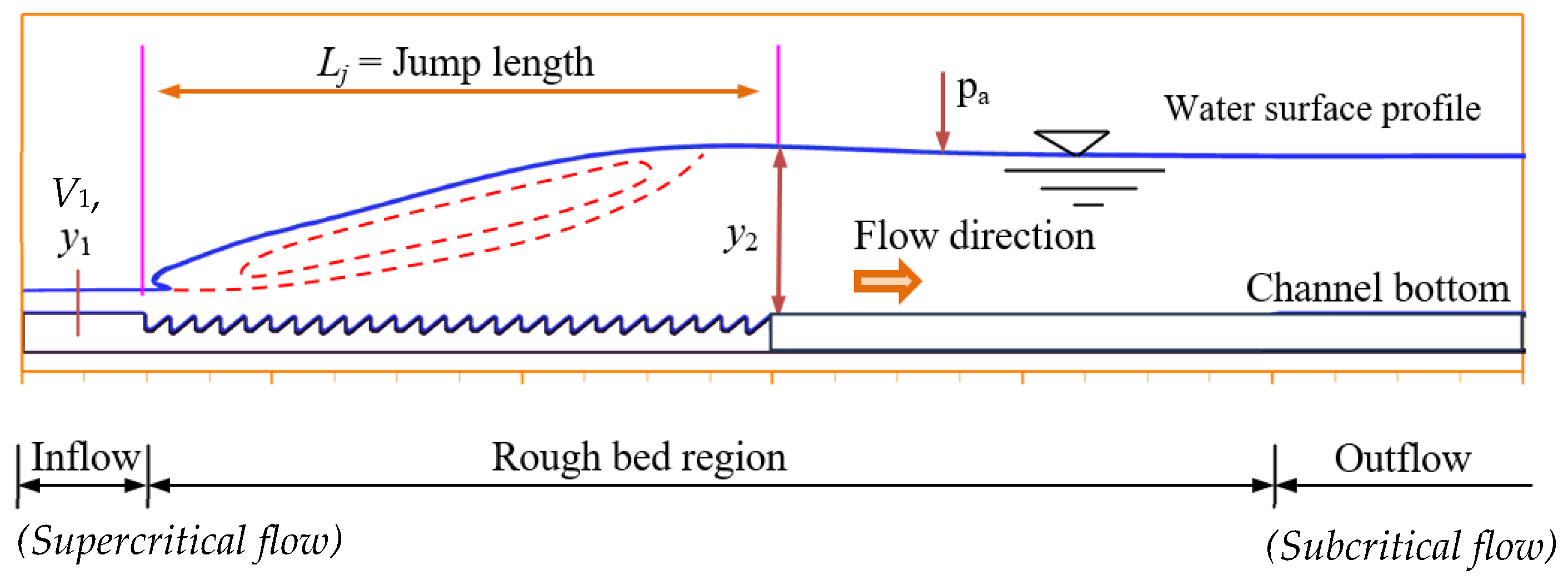
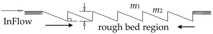
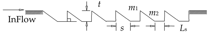
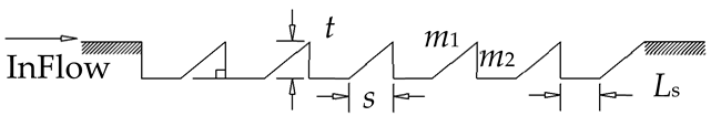
Based on physical models reported by Samadi-Boroujeni, H. et al. [4], this study proposes four rough bed models designed and studied with numerical models by modifying the geometry characteristics of triangular rough elements and their arrangement on the channel bottom, simultaneously expanding the study range for flow conditions and also their geometry (see Table 1), with the aim to improve the hydraulic jump characteristics of rough beds compared with previous research. The hydraulic jump characteristics on a right triangular prism rough bed are illustrated in Figure 1.

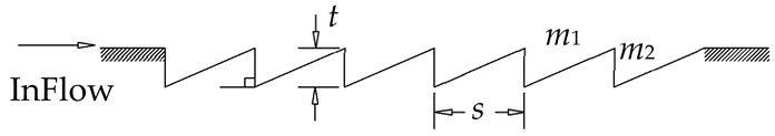
Table 1.
Schematic of rough beds using the simulations and study parameters.
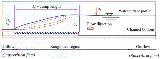
Figure 1.
Hydraulic jump on a right triangular prism rough bed.
2.2. Dimensional Analysis for Hydraulic Jump Characteristics
The conjugate depth (y2) and jump length (Lj) are the two main parameters of the hydraulic jump phenomenon that directly affect the scale and cost of the stilling basin construction. Therefore, these parameters must be clearly defined in the design of irrigation works. Therefore, this section presents how to determine the relationship between these parameters, the upstream flow conditions, and the geometry characteristics of a rough bed configuration. Those relationships might be written as the following:
where ρ, ν, and g are the mass density of water, water kinematic viscosity, and gravity acceleration; m1 and m2 are the upstream and downstream slope of roughness element, and V1 is the inflow velocity.
In this study, we chose three repeated variables, including supercritical flow depth y1, initial flow velocity V1, and density of water ρ, to perform a dimensionless analysis for both parameters y2/y1 and Lj/y1. With the initial Reynolds number (27.3 × 10³ ≤ Re1 ≤ 151.8 × 10³), the viscosity effect was neglected. By using the Pi theorem, Equation (1) can be rewritten as follows:
Similarly, we also obtained the relationship of energy loss (EL/E1) and shear force coefficient (εf) with flow conditions and rough bottom geometry as follows:
2.3. Numerical Flow-3D Model Theory
This paper used the CFD method to simulate the hydraulic jump phenomenon over right triangular prism rough beds by combining the volume of fluid (VOF) method and the RNG k-ε turbulent model. The RNG k-ε turbulent model is more accurate than the standard k-ε model for simulating hydraulic jumps on rough beds because it can consider the effect of small-scale vortex motion [5,13]. The volume of fluid (VOF) method is a free-surface modeling approach, i.e., a numerical method for tracking and locating the free surface (air–fluids interface) [3,5,6,13,14,15]. Equations utilized in this CFD technique include continuity and momentum equaitons expressed as:
where t is time; ui and uj are velocity components; xi and xj are coordinate components; μ is the molecular viscosity coefficient; μt is the turbulent viscosity coefficient; and P is the hydrostatic pressure.
Equations for the RNG k-ε turbulent model are
where k is the turbulent kinetic energy; ε is the turbulent dissipation rate; Gk is the production of turbulent kinetic energy, the constants: σk, σε, C1ε, and C2ε is introduced by Yakhot and Orszag [16].
The VOF transport [17] equation is described by Equation (6). Here, F denotes the fraction function. A free surface must be cells having F values between unity and zero.
where VF is the flow volume; and Ax, Ay, and Az are the flow areas.
2.4. Entropy Production by Dissipation
The specific entropy production rate can be defined as Equation (7) [18].
where represents the energy transfer rate. In a steady state, is equal to the dissipation energy; and T is the temperature.
For turbulent flows, after time-averaging of the entropy production by dissipation, two groups of terms appear, one caused by time-averaged movement and another caused by velocity fluctuations. Then, can be expressed as [19,20]:
where and represent the particular entropy production rate due to the time-averaged movement and the specific entropy production rate due to velocity fluctuations, which can be calculated as follows:
where denotes the dynamic viscosity; stands for the turbulent viscosity; , , and are time-averaged velocity components; , , and are velocity fluctuation components; and µeff represents the effective viscosity ().
Equation (9) represents the entropy production by dissipation in the mean flow field, referred to as direct dissipation. Meanwhile, Equation (10) is the so-called indirect or turbulent dissipation.
2.5. Define Computational Grid and Boundary Conditions for Numerical Simulations
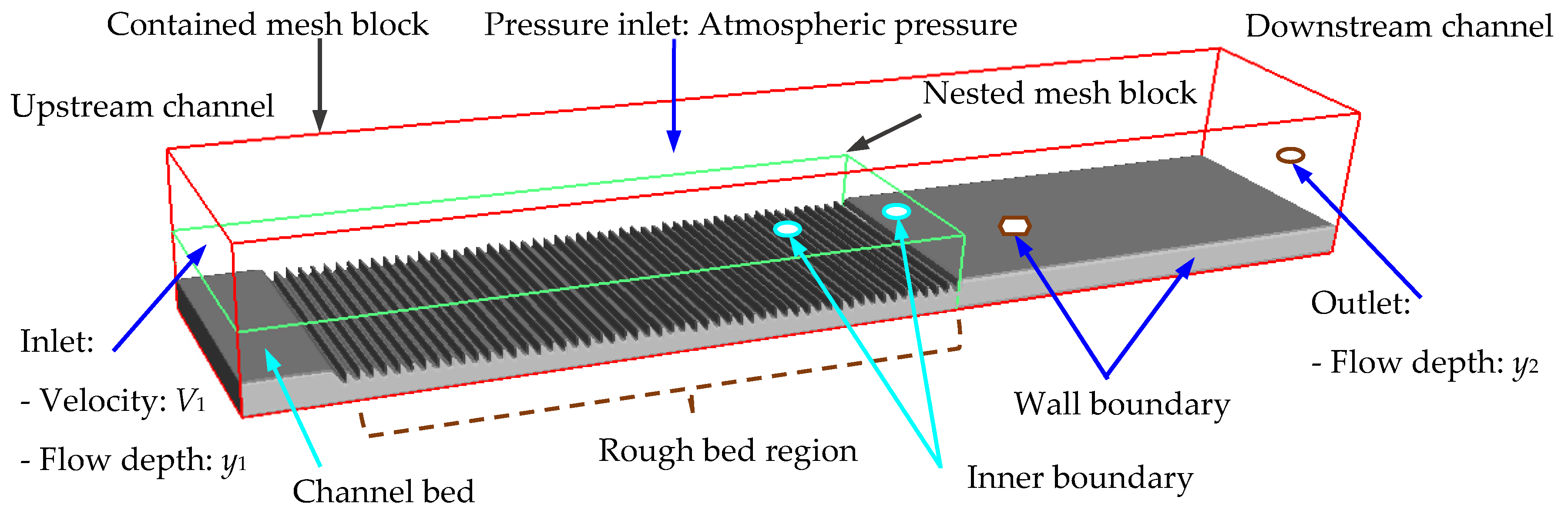
In this research, the calculated domain of the numerical models is made up of two mesh blocks (see Figure 2). The contained mesh block was set up for the whole numerical model space; meanwhile, the rough bed region is set by the nested mesh block because these regions need a finer mesh to capture the flow behavior better. A structured grid with the same three-dimensional grid size was used in these numerical models. This study also considers three computational grids (see Table 2) to evaluate the calculated grid independence for the numerical result, determine the appropriate grid size for the best steady numerical results, and apply this grid to the subsequent simulations.
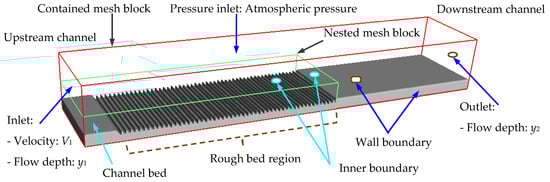
Figure 2.
Boundary conditions are applied for a calculated domain.
Table 2.
Characteristics of the computational grids.
Based on the experimental data reported by Samadi-Boroujeni, H. et al. [4], the boundary condition of the numerical models was set up as shown in Figure 2: The inlet boundary condition (upstream channel) simultaneously assigns velocity V1 and supercritical depth y1. The outlet boundary is set at the water level with a subcritical depth of y2. The free surface boundary condition provides the atmospheric pressure. The channel bottom is a wall boundary, and symmetry boundary conditions provide the inner boundary conditions.
This paper uses the grid convergence index (GCI) method, which is introduced and recommended by Celik and Ghia [21], to evaluate calculated grid independence, as described in Equation (11).
where the value of p is equal to 10.76 and is called the accuracy local order; are the calculation result and grid size of the i-th grid, respectively, and satisfy the relationship of ; and i was taken by 1 and 2 only.
The variable is used to judge mesh convergence. The variable value is assigned to y2/y1 (sequent depth ratio), which changes with different calculated meshes. In this research, we use the numerical result of the rough bed M_II model for the No.82 test (with initial conditions such as y1 = 0.02 m and Fr1 = 5.65). The results of the mesh convergence analysis are shown in Table 3. In this table, the GCI21 value equals 0.031 percent, which is considered very small.
Table 3.
The mesh convergence analysis for calculated grids.
On the other hand, to verify that the numerical results are unique and accurate, a suitable mesh size needs to be chosen. This article compares the Lj/y1 jump length ratio values obtained from two types of grids, Grid 1 and Grid 2. Table 4 shows the results of the jump length ratio (Lj/y1) between Grid 1 and Grid 2, with errors less than 5%. Therefore, Grid 1 and Grid 2 almost satisfy the grid’s independence. Based on the efficiency, accuracy, and computation time of numerical simulation results, Grid 2 is used for all subsequent simulations.
Table 4.
Comparison of jump length results between Grid 1 and Grid 2.
3. Results and Analysis
3.1. Validation of the Numerical Simulation Models
Based on the experimental data of Samadi-Boroujeni, H. et al. [4], this simulation used the conjugate depth ratio (y2/y1) and the jump length ratio to confirm the CFD model. As mentioned, Grid 2 was used to run numerical simulation cases from the experimental data. In this paper, the Sheet II tests were chosen to validate the CFD model with the specific parameters for the conducted experiments, as shown in detail in Table 5.
Table 5.
Primary details of conducted experiments [4].
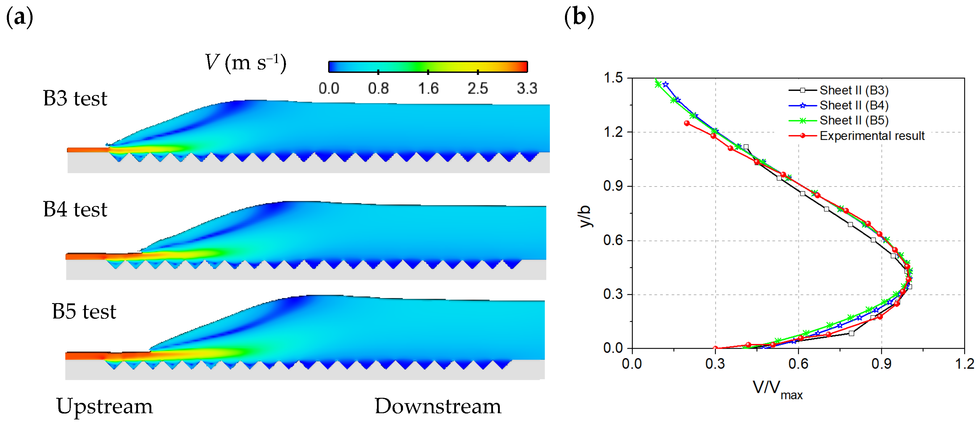
Table 6 shows the experimental comparison with the simulation model data for hydraulic jumps, with a relative error of less than 5%. The error may be due to the measurement error and boundary layer effects. On the other hand, Figure 3 shows that the normalized forward flow velocity profile between numerical simulations and experimental results agrees well. It shows that the numerical results correlate well with the experimental data by Samadi-Boroujeni, H. et al. [4]. Thus, the reliability of the numerical model is validated.
Table 6.
Comparison of numerical and experimental results for hydraulic jumps.
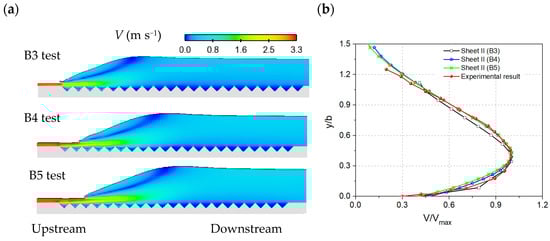
Figure 3.
(a) Velocity field, (b) normalized velocity profile forward flow in hydraulic jumps.
This study has performed 210 numerical simulation cases for right triangular prism rough beds. The numerical simulation results defined the hydraulic jump characteristics, such as the sequent depth and jump length with different arrangements of rough beds and flow conditions, which are summarized in the following (Table 7).
Table 7.
Numerical results for a hydraulic jump on right triangular prism rough beds.
3.2. Water Surface Profiles on Hydraulic Jumps
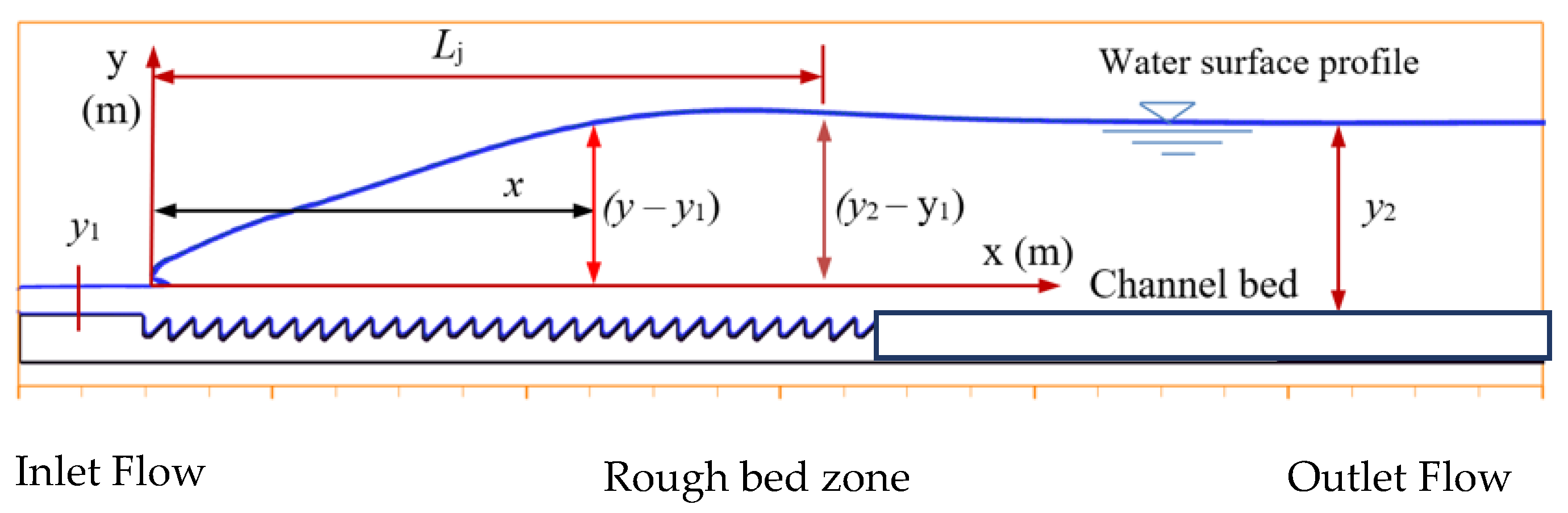
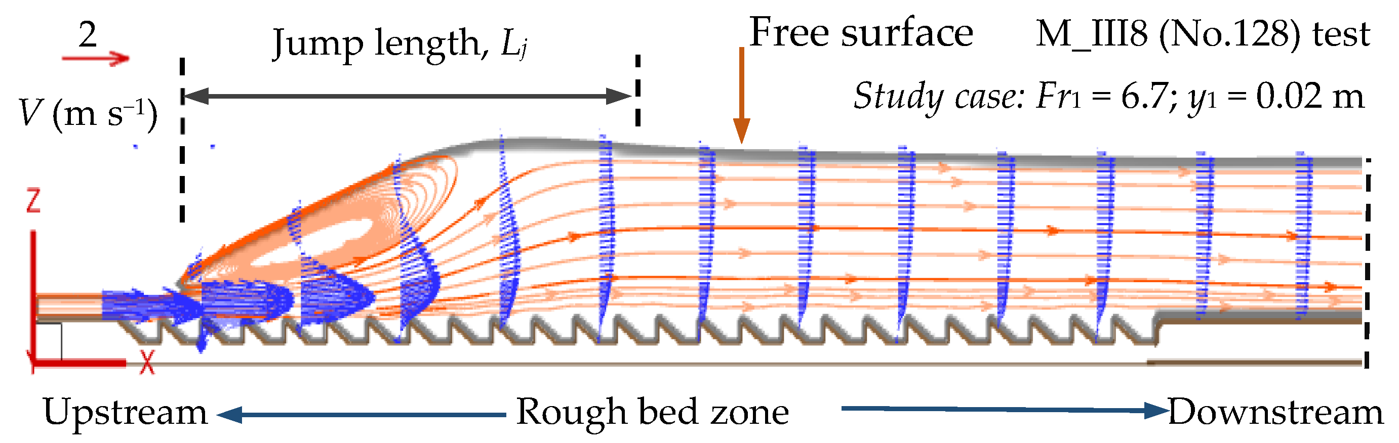
The water surface profiles in this numerical simulation are determined by the VOF method. The water surface profiles in these simulations help design an efficient construction of the stilling basin’s side wall heights and floor lengths. The coordinate system for defining the water surface profiles is described and shown in Figure 4. These numerical results of a typical free surface elevation on M_I and II bed models are presented in Figure 5.
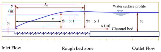
Figure 4.
Describe the Water surface profile on a hydraulic jump.
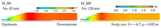
Figure 5.
Describe the free surface elevation contours for rough beds.
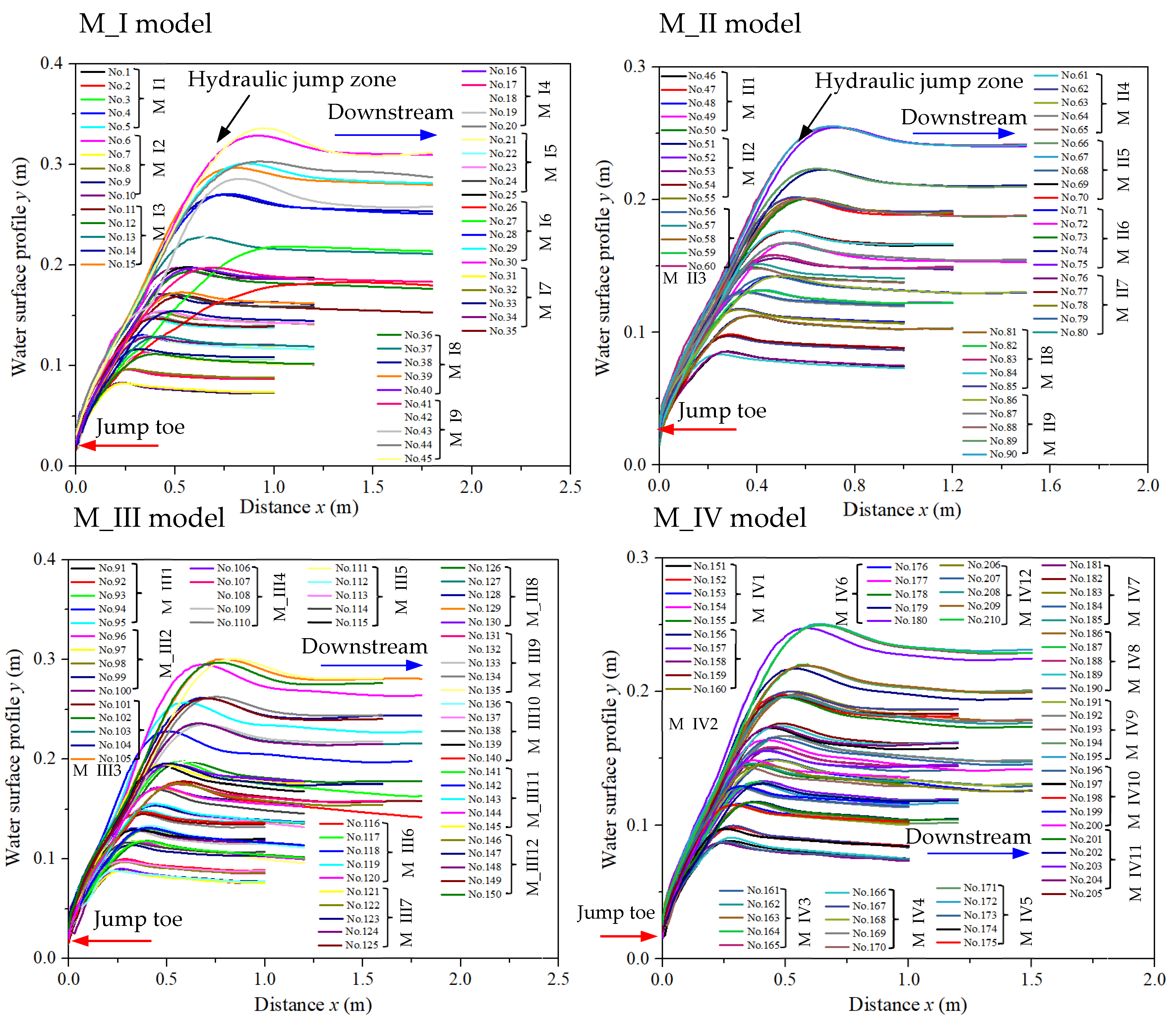
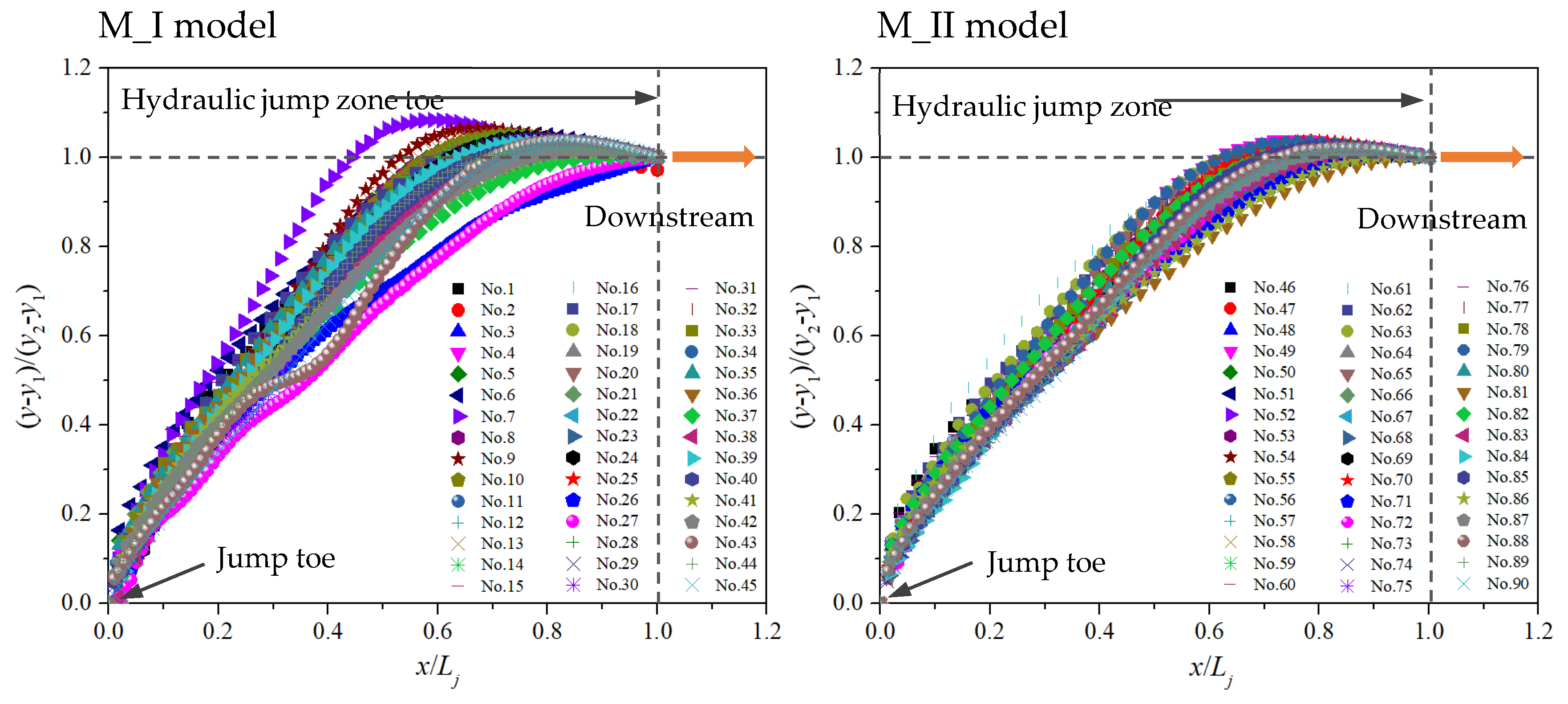
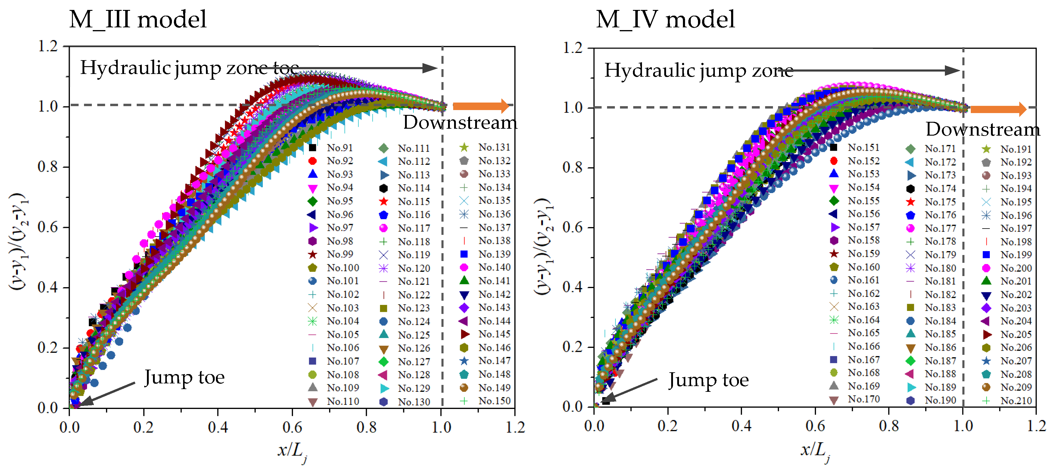
The water surface profiles are illustrated in Figure 6. These figures clearly describe the hydraulic jump and downstream regions. In there, jump toes are at the start points of the right triangular prism rough beds. In addition, the water surface profiles for the hydraulic jump region are also detailed in Figure 7, indicating that the normalized water surface profiles on different rough beds are also nearly similar.
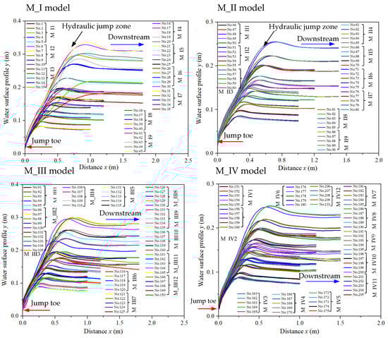
Figure 6.
Water surface profiles on the different rough bed models.
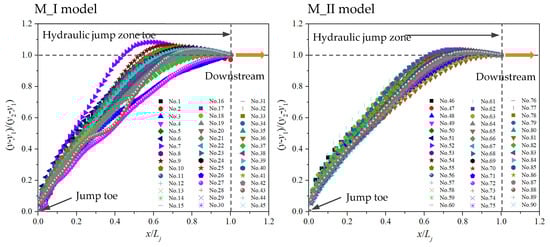
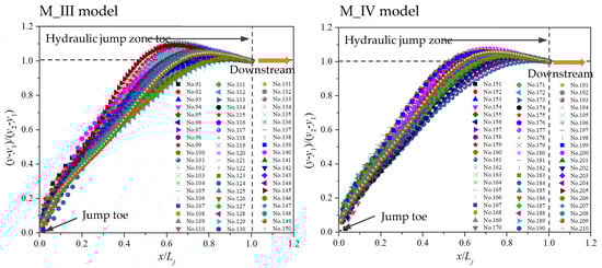
Figure 7.
Normalized water surface profiles for the hydraulic jump region on rough bed models.
3.3. Effects of Right Triangular Prism Rough Beds on Sequent Depth Ratio
The conjugate depth y2 is the basis for defining the stilling basin side wall’s height to help reduce the downstream flow influence on the riverbank. Through Table 7, the values of the conjugate depth ratio y2/y1 were calculated for all numerical cases. Based on Equation (2) and the multiple linear regression method (MLR), this study found a relationship between the sequent depth ratios, the shape factors of the right triangular prism rough beds, and inflow conditions (see Equation (12)).
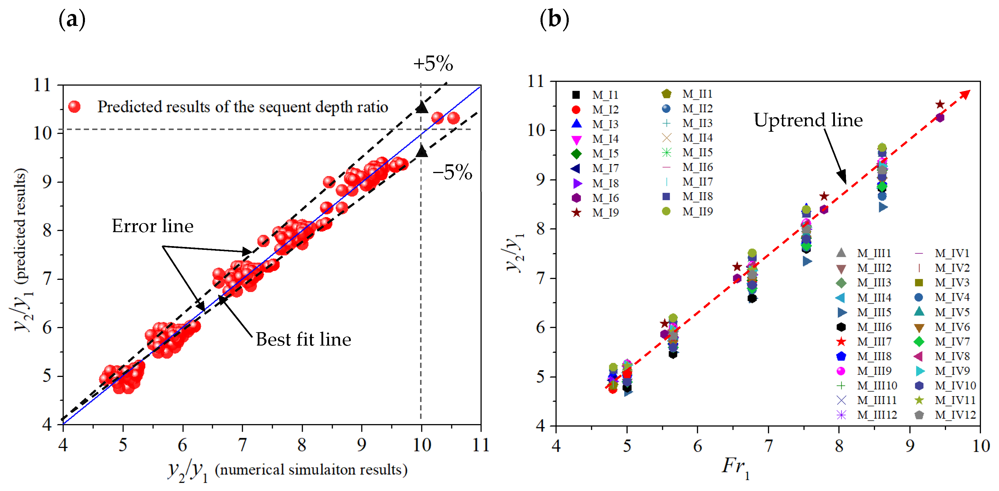
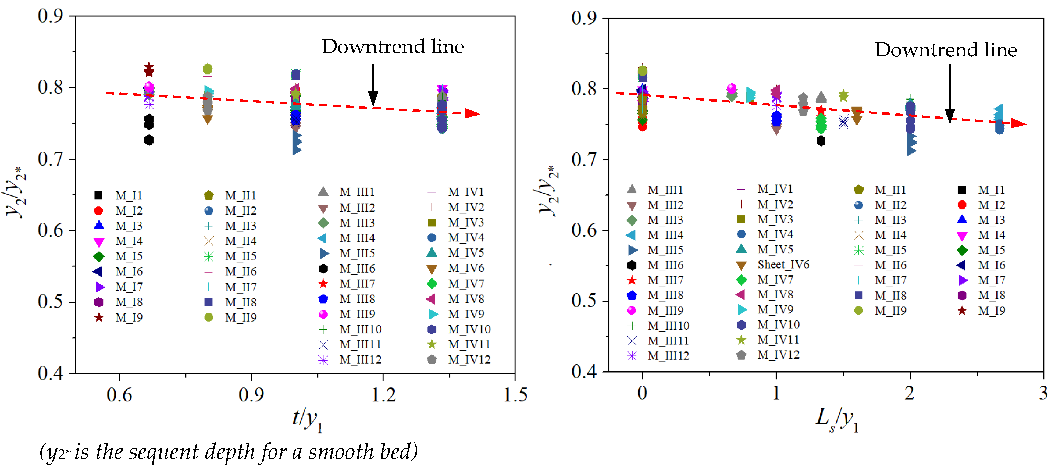
Equation (12), which obtained a very high correlation coefficient of 0.987, indicated that the y2/y1 predicted results agreed with the y2/y1 value from numerical simulation results (error < 5%), as shown in Figure 8a. From Equation (12), the y2/y1 values were strongly dependent on Fr1 (see Figure 8b), which is understood when supercritical flow changes to subcritical flow through the hydraulic jump phenomenon. On the contrary, the two parameters (t/y1 and Ls/y1) decrease with the sequent depth ratio, as shown in Figure 9. According to MLR analysis results, the upstream and downstream slopes of triangular roughness (m1,2) have a minimal effect on the increase in sequent depth ratio. Thus, it is absent in Equation (12). This could be explained by the variation in the flow field in the hydraulic jump zone and the small eddy structures that appear within the rough bed range (analyzed in detail in Section 3.7).
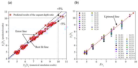
Figure 8.
(a) predicted versus numerical results of y2/y1; (b) y2/y1 versus Fr1 for rough beds.
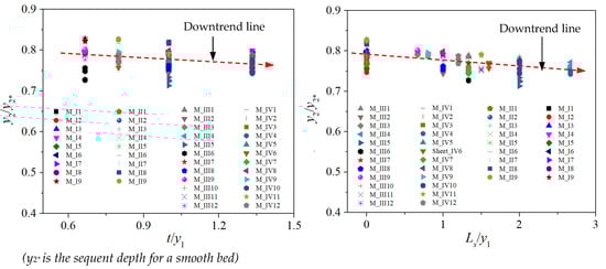
Figure 9.
y2/y2* versus t/y1 and Ls/y1 for all rough bed models.
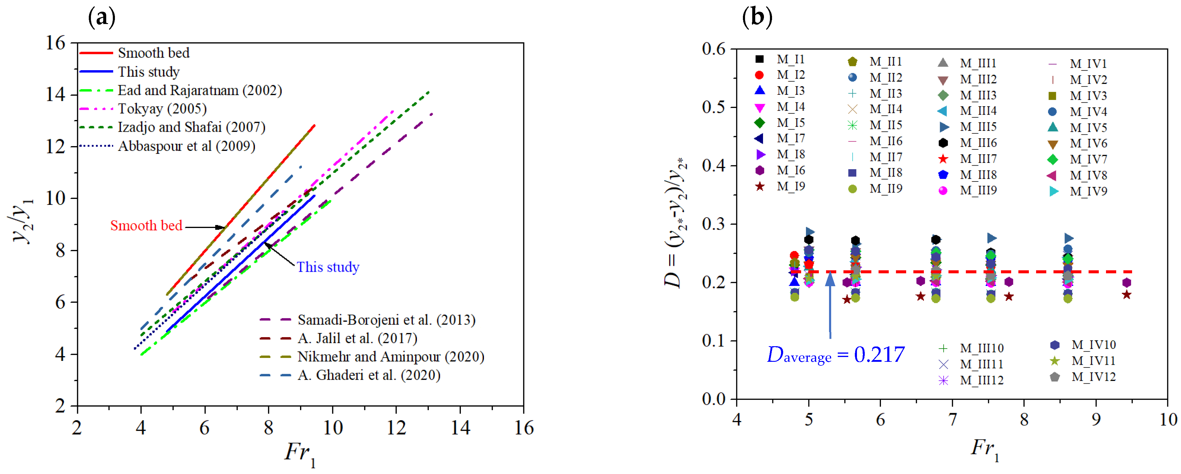
Figure 10a plots this study’s depth ratios (y2/y1) and earlier studies versus Fr1. This figure shows that the depth ratio y2/y1 for the rough beds is smaller than the smooth bed (classical jump). Therefore, the effect of the right triangular prism rough beds reduces in comparison with the conjugate depth. The results of this study also indicate a good agreement with those obtained by previous studies [1,2,5,7,8,13].
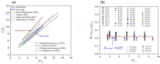
Figure 10.
(a) y2/y1 values versus Fr1 for this study and other works; (b) D values versus Fr1 for rough beds [1,2,4,5,7,8,9,13].
This research uses the D = (y2* − y2)/y2* parameter introduced by Ead and Rajaratnam [1] to define the reduction in the conjugate depth between rough and smooth beds. The variation in the D parameter against Fr1 is shown in Figure 10b. The D parameter has an average value of 0.217, indicating that hydraulic jumps on the rough beds provide a conjugate depth after the jump that is approximately 21.7 % less than the smooth bottom.
On the other hand, Figure 10b also shows that the M_III and VI models effectively reduce the conjugate depth better than the M_I and II models. The maximum D value is 0.287 for the M_III model with Fr1 = 5.0, and the minimum is 0.171 for the M_I model with Fr1 = 5.65. The findings of this study are in good agreement with those of Ead and Rajaratnam [1], Tokyay [7], and Izadjoo and Shafai-Bejestan [8]. They are about 0.25, 0.2, and 0.2, respectively.
3.4. Effects of Right Triangular Prism Rough Beds on Jump Length Ratio
The stilling basin’s length depended on the jump length, which determined the channel bed’s reinforcement range to prevent erosion during flood drainage work operations. Based on the water surface profiles and velocity field in all numerical simulation results, we could define the jump length Lj as illustrated in Figure 11 below:
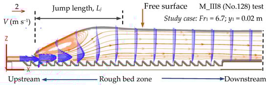
Figure 11.
Describe the hydraulic jump length on rough beds.
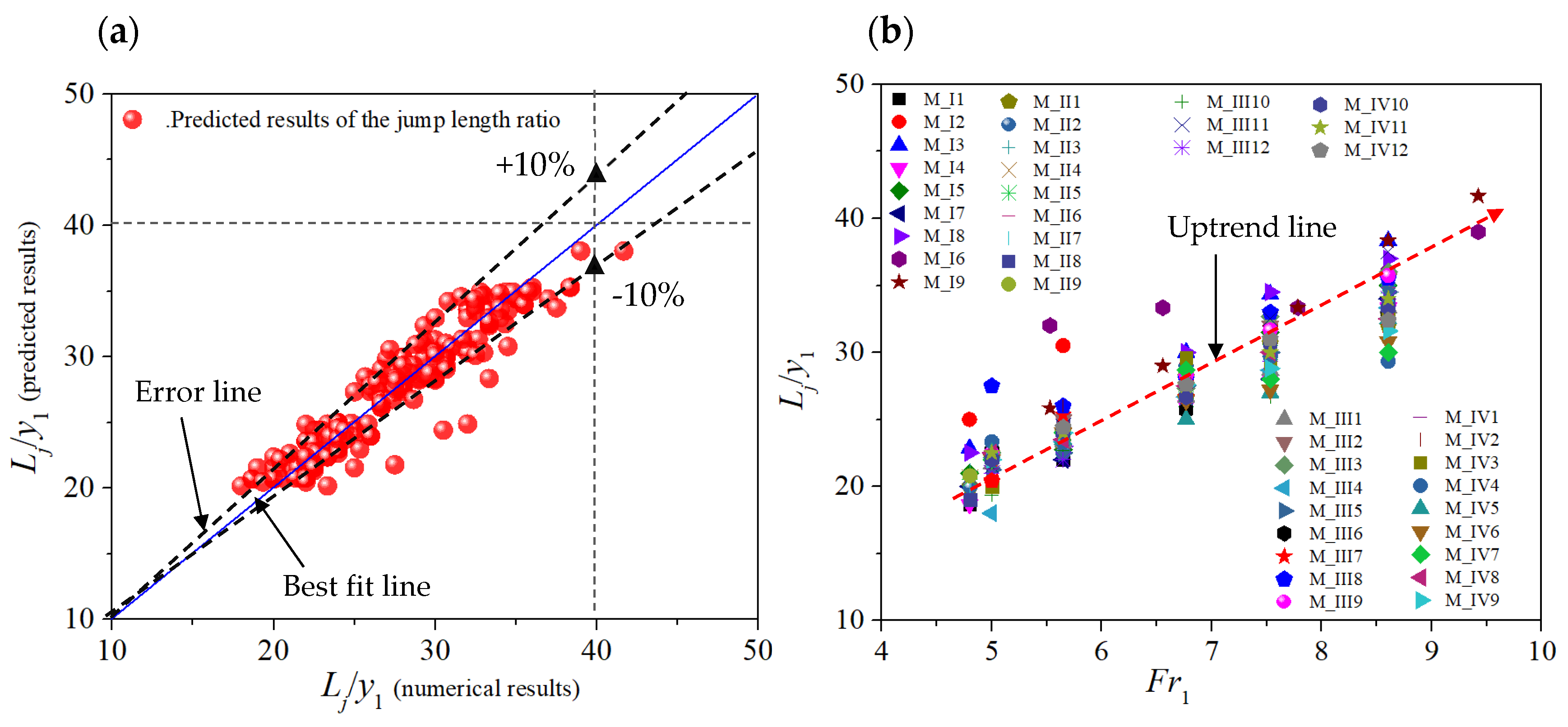
Through the jump length data described in Table 7 and combined with the MLR method and Equation (2), this study found Equation (13) with a high correlation coefficient of 0.89.
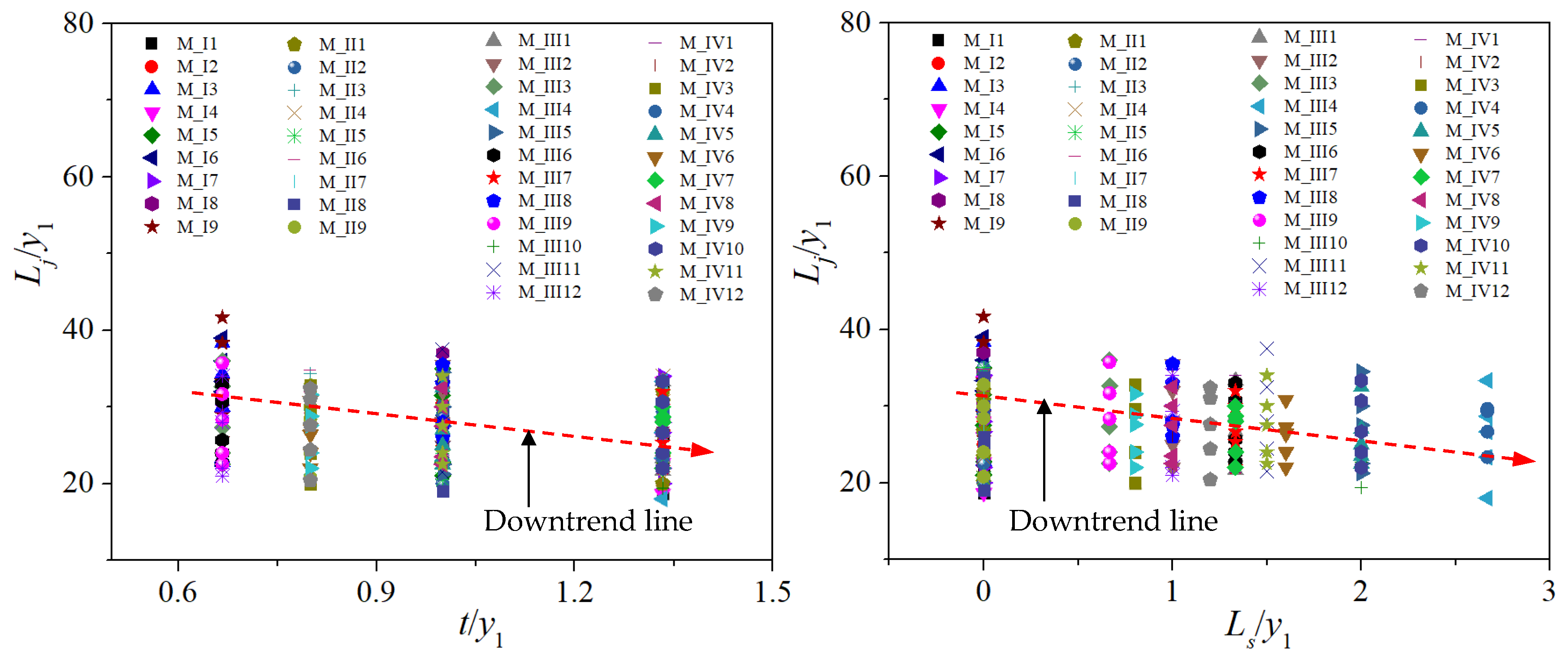
The predicted results of the Lj/y1 parameter by Equation (13) were compared with the numerical simulation results, as shown in Figure 12a. In this figure, the Lj/y1 values were predicted quite accurately (error < 10%) with the Lj/y1 numerical simulation values. On the other hand, from Equation (13), the jump length is most dependent on Fr1. It means the supercritical flow with a larger Fr1 needs more jump length to change from supercritical to subcritical flow (see Figure 12b). Meanwhile, the two geometry parameters (t/y1, Ls/y1) have a negligible effect on reducing the jump length ratio, as shown in Figure 13.
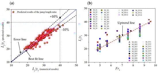
Figure 12.
(a) predicted versus numerical results of Lj/y1, (b) Lj/y1 versus Fr1 for rough beds.
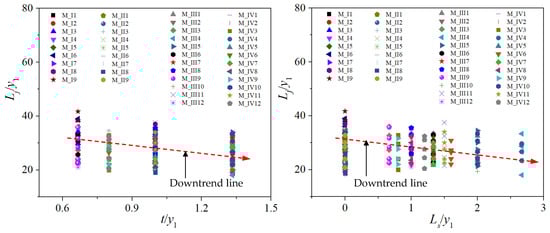
Figure 13.
Lj/y1 versus t/y1 and Ls/y1 for all rough bed models.
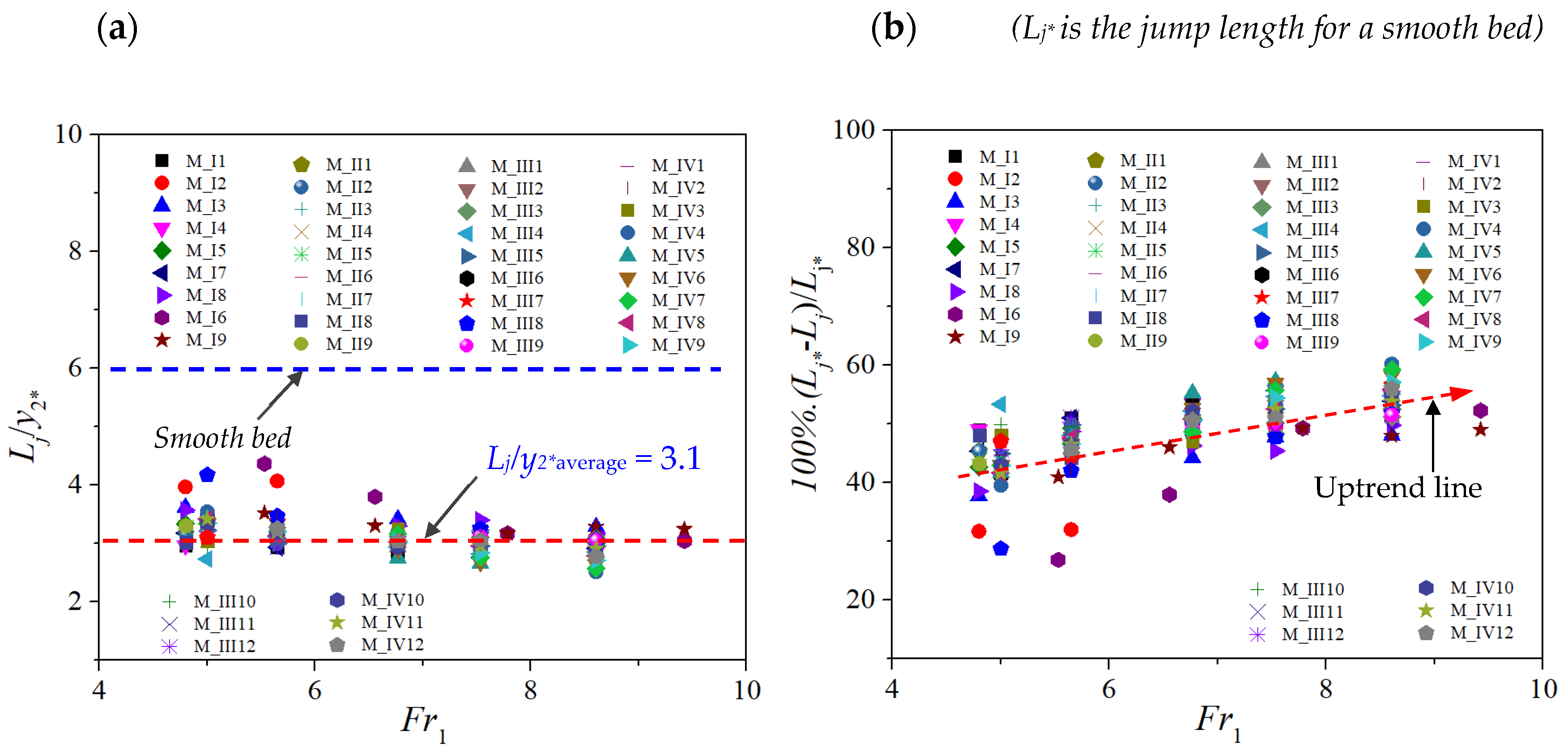
Figure 14a shows the dimensionless jump lengths Lj/y2* versus the upstream Froude number Fr1. This figure indicates that the right triangular prism rough beds strongly decrease the jump length compared with the smooth bed. More specifically, the Lj/y2* value was about 3.0 for initial Froude numbers greater than 6.8 and about 3.2 for initial Froude numbers smaller than 6.8. It means the jump length on various rough beds was approximately 50% shorter than on smooth ones (see Figure 14b). The findings of this study are in good agreement with those of Ead and Rajaratnam [1], Tokyay [7], Abbaspour and Dalir [2], and Samadi-Boroujeni, H. et al. [4]. They are about 3, 4, 3.2, and 3, respectively.
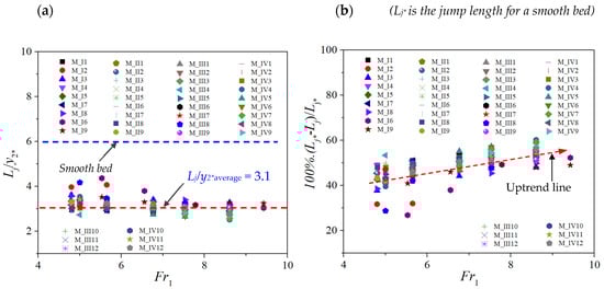
Figure 14.
(a) Lj/y2* versus Fr1 for rough models; (b) Variation of jump length between rough and smooth beds versus Fr1.
Figure 14b also indicates that the M_III and VI models reduce the jump length better than the M_I and II models. M_I model has the lowest effective jump length reduction with a small Fr1.
3.5. Effects of Right Triangular Prism Rough Beds on Energy Loss
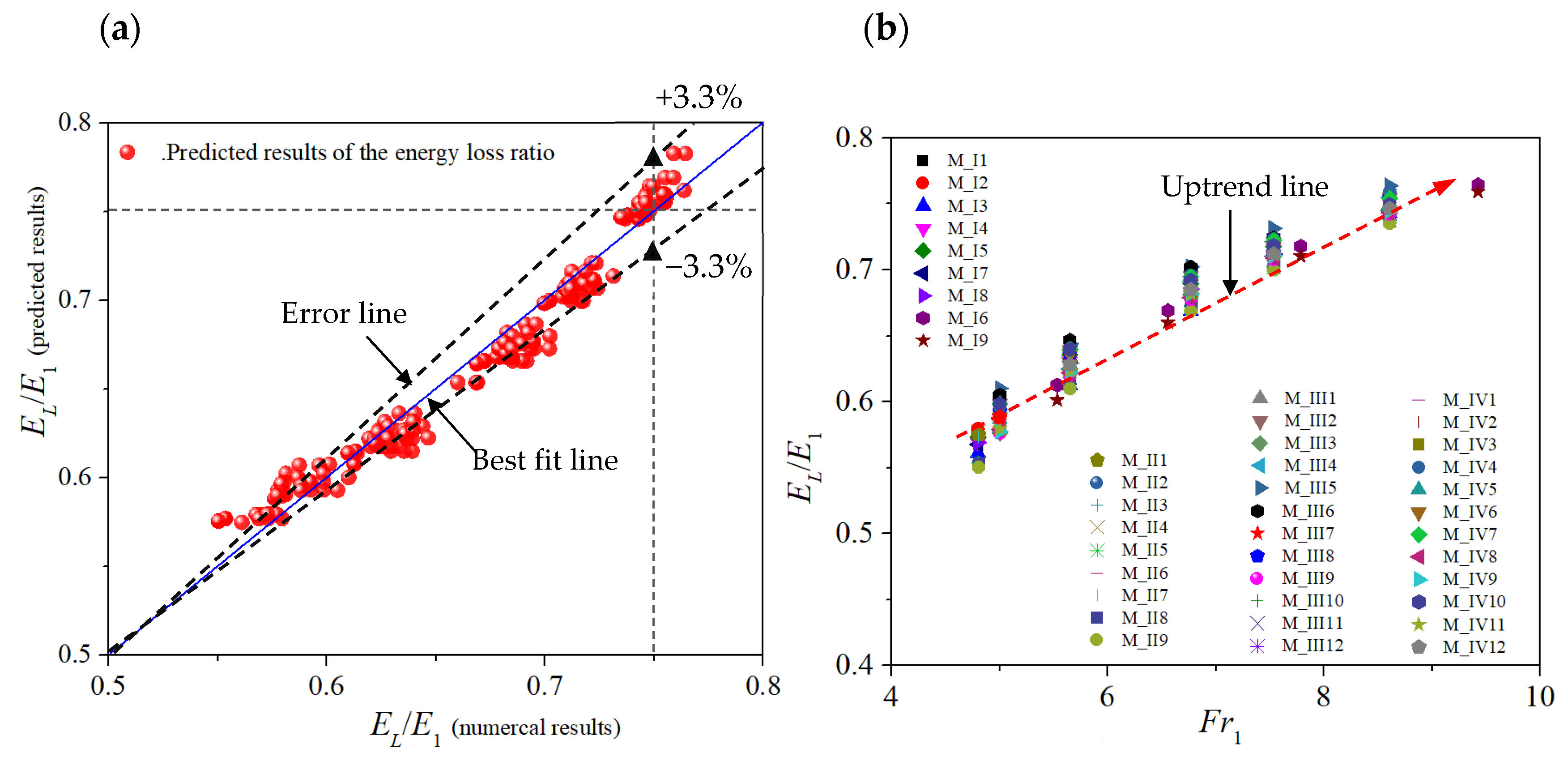
A stable and free hydraulic jump is characterized by significant energy dissipation. Therefore, we need to evaluate the variation in the energy loss through hydraulic jumps. The energy loss values were calculated as the difference in flow energy before and after the jump from data from the numerical simulation results (see Table 7). Using the MLR method, combined with Equation (3), this research found the energy loss ratio EL/E1 relative to the parameters of inflow conditions and roughness configuration can be written as:
Equation (14) shows that the parameter EL/E1 had an extreme variation versus Fr1. When the Fr1 value increases, then the energy loss value also increases (see Figure 15a). At the same time, two geometries of the rough bed parameters (t/y1, Ls/y1) had minor effects on increasing the energy loss ratio (see Figure 16). In addition, Figure 15a also, once again, shows that the EL/E1 values predicted by Equation (14) agreed with the EL/E1 values from numerical simulation results (error < 5%).
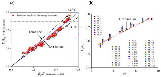
Figure 15.
(a) Predicted versus numerical results of EL/E1, (b) EL/E1 parameter against Fr1.
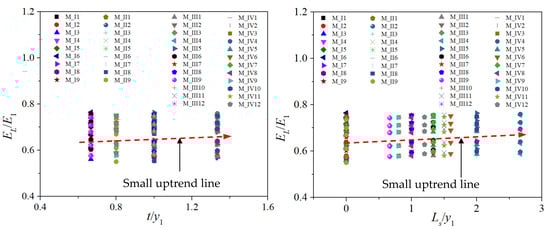
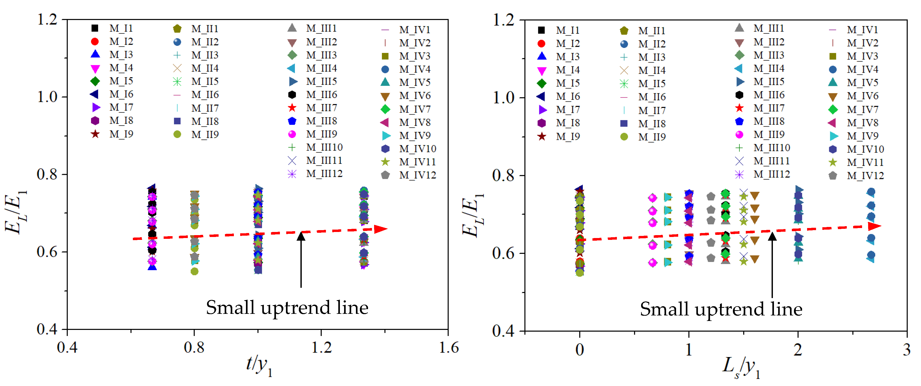
Figure 16.
EL/E1 versus t/y1 and Ls/y1 for all rough bed models.
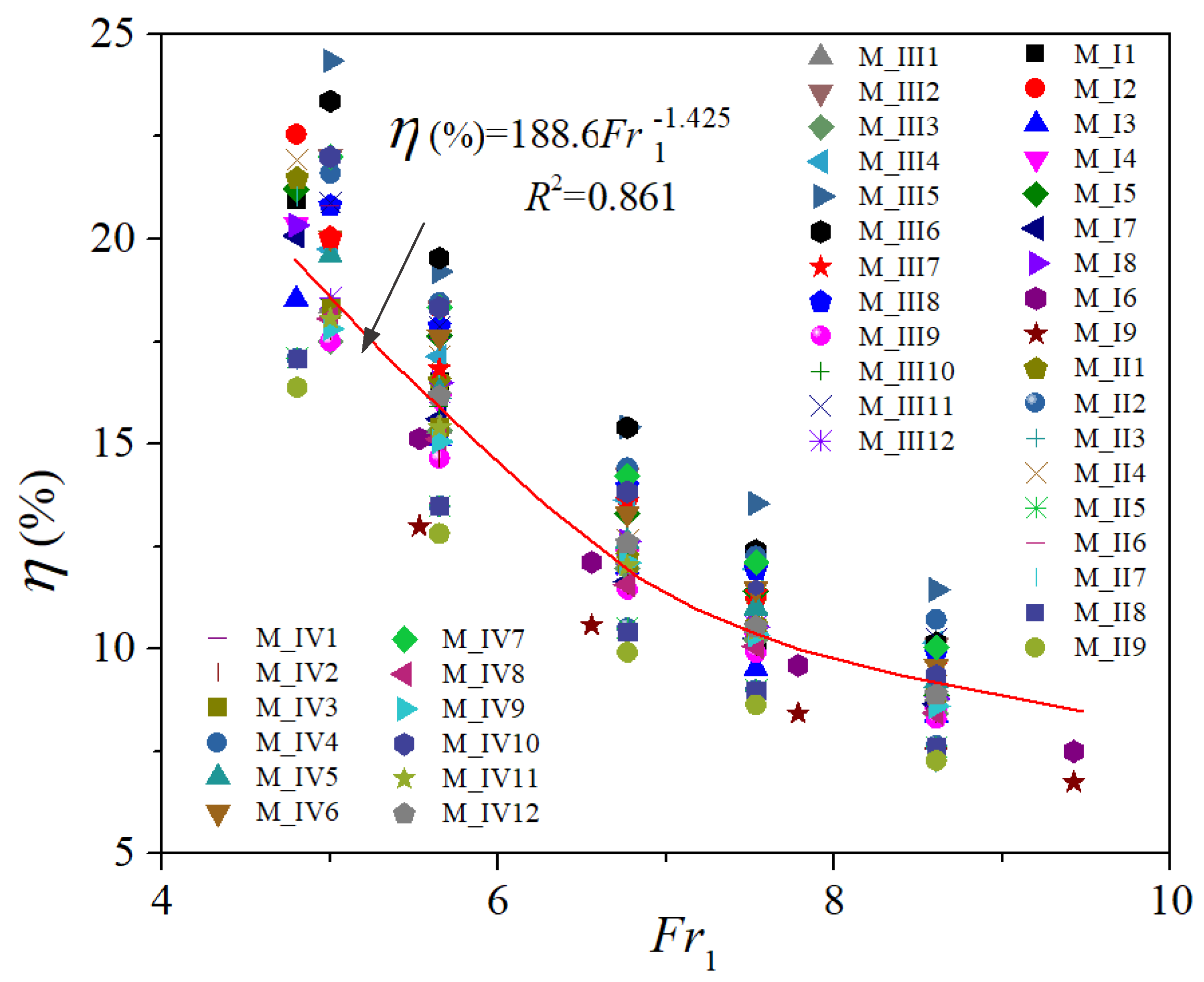
This research uses the η parameter to evaluate the energy loss of the flow through the hydraulic jump zone. It is determined by the formula as follows: η = (EL − EL*)/EL* where EL* is the energy loss for smooth beds. Based on the numerical simulation results for different rough bed models, this study found a relationship between energy loss and the Fr1 parameter as follows:
Figure 17 shows the η values versus Fr1 parameters. This figure indicated that the right triangular prism rough beds used in this study had increased the energy loss in flow. In more detail, the increase in energy loss varies from 4% to 24% compared with smooth beds at the same initial Froude number condition. Therefore, these rough beds improve the flow’s energy dissipation in the hydraulic jump region.
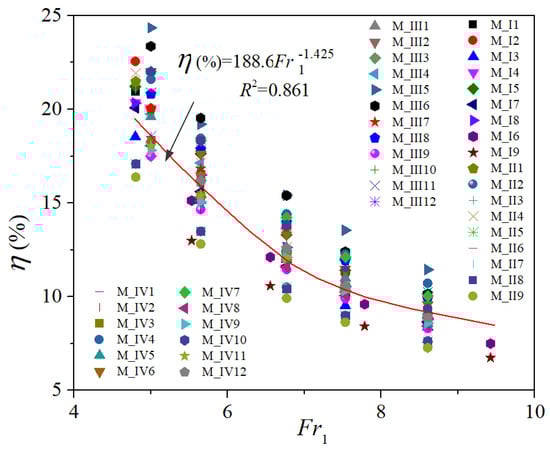
Figure 17.
Variation in the η energy loss parameters versus Fr1 for all rough bed models.
3.6. Evaluate Variation in the Bed Shear Stress for Rough Beds
Increased bed shear stress is one of the primary reasons for the reduction in conjugate depth and the length of the hydraulic jump over the rough beds. The shear force coefficient εf [1] mentioned in this section was determined as follows:
where P1, P2, M1, and M2 are the hydrostatic pressure force and momentum flux per unit width at the sections before and after the jump, respectively [22].
Based on the numerical model results data, as shown in Table 7, this study calculated the εf values by Equation (16). We used the MLR method to find a relationship between the εf parameter, geometry characteristics of rough beds, and inflow conditions, which is written below.
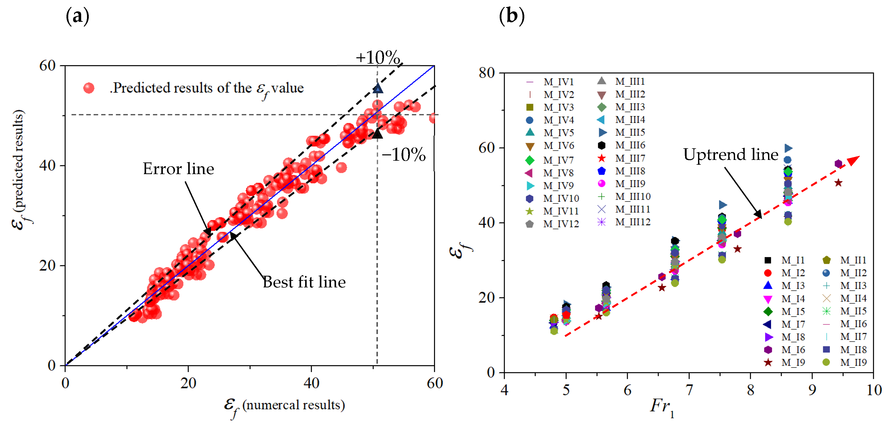
The εf predicted values calculated by Equation (17) are compared with the εf numerical simulation result values, as shown in Figure 18a. This figure shows that the εf values calculated by Equation (17) entirely agree with the numerical result values with an error of <10%. Equation (17) demonstrates that the εf values are strongly dependent on Fr1 parameters. On the contrary, the two parameters (t/y1, Ls/y1) have a negligible effect on increasing the bed shear stress, as shown in Figure 19.
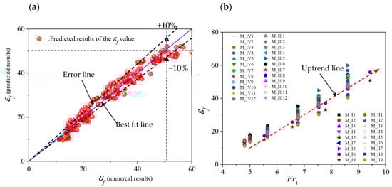
Figure 18.
(a) Predicted versus numerical results of εf, (b) εf parameter against Fr1.
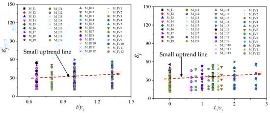
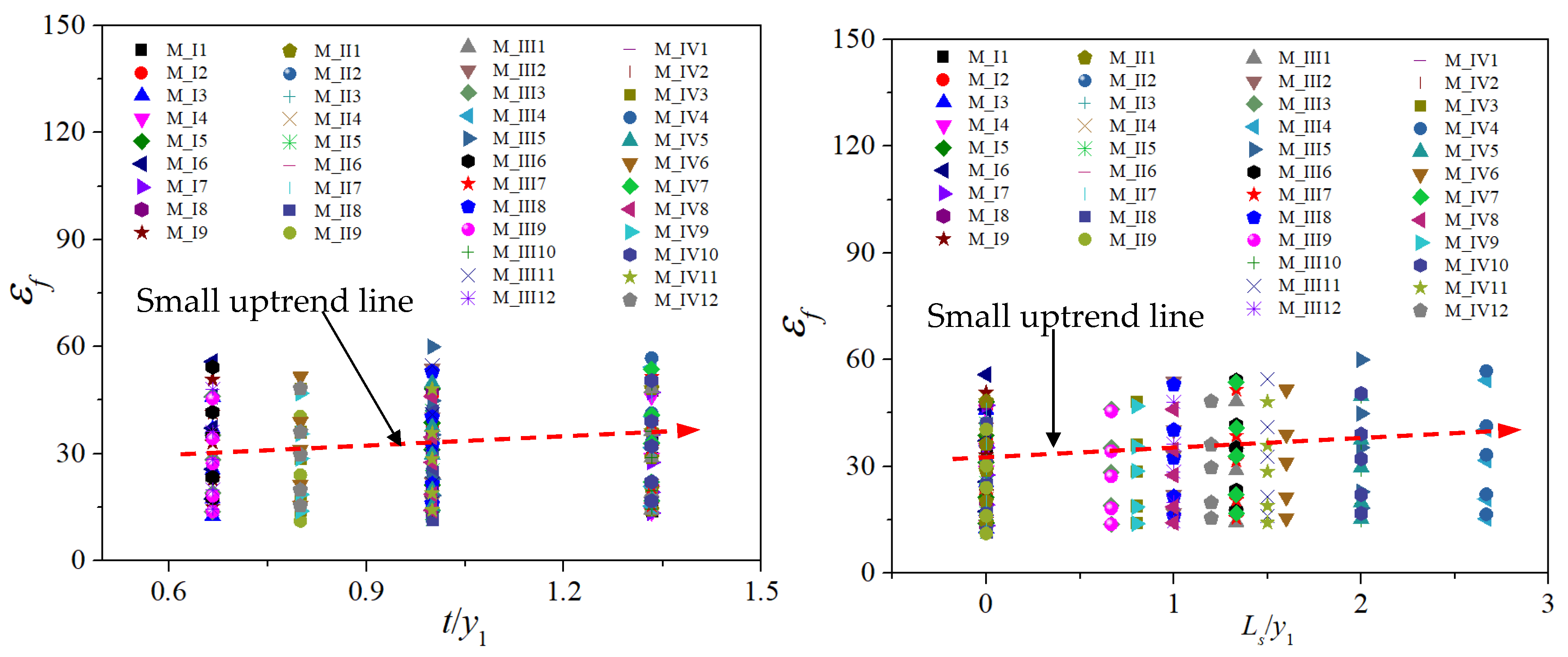
Figure 19.
The εf values versus t/y1 and Ls/y1 for all rough bed models.
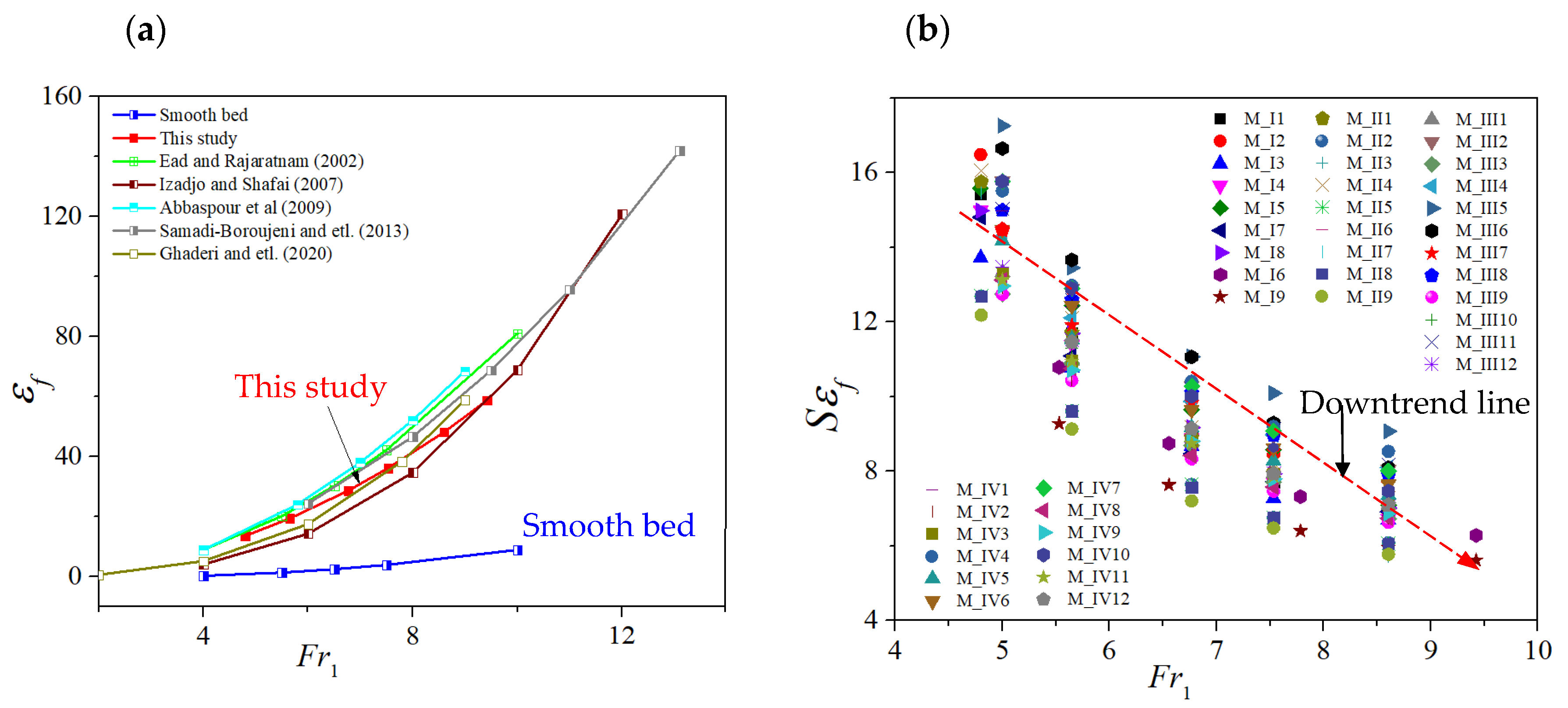
In Figure 20a, the shear force coefficient εf was plotted versus inlet Froude numbers Fr1 for other works. This figure shows good agreement between this study’s and previous researchers’ results. On the other hand, Figure 20b shows that the number of εf hydraulic jumps over the right triangular prism rough beds is almost ten times that of the bed shear stress in jumping over the smooth bed, and it can be written by the equation below:
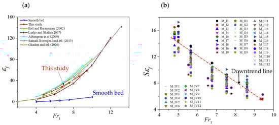
Figure 20.
(a) Variation in the εf values with Fr1 for other works, (b) Variation in the surplus of shear force factor with Fr1 [1,2,4,5,8].
The values of the shear force coefficient surplus parameter versus the inlet Froude numbers are shown in Figure 20b. This figure shows that the maximum value of is equal to 17.3 with Fr1 = 5.0 for M_III model, and the minimum value of is equal to 5.5 with Fr1 = 9.4 for M_I model. This research indicates that the value of εf is more significant when the models are placed with a discontinuous roughness element on the channel bed compared to when they are arranged with a continuous roughness element. Additionally, the shear force coefficient of the rough bed models analyzed in this research is about ten times greater than that of the smooth bed models under the same test conditions. ( is the shear force coefficient of a classical jump).
3.7. Effects of Right Triangular Prism Rough Bed on Total Entropy Generation Rate
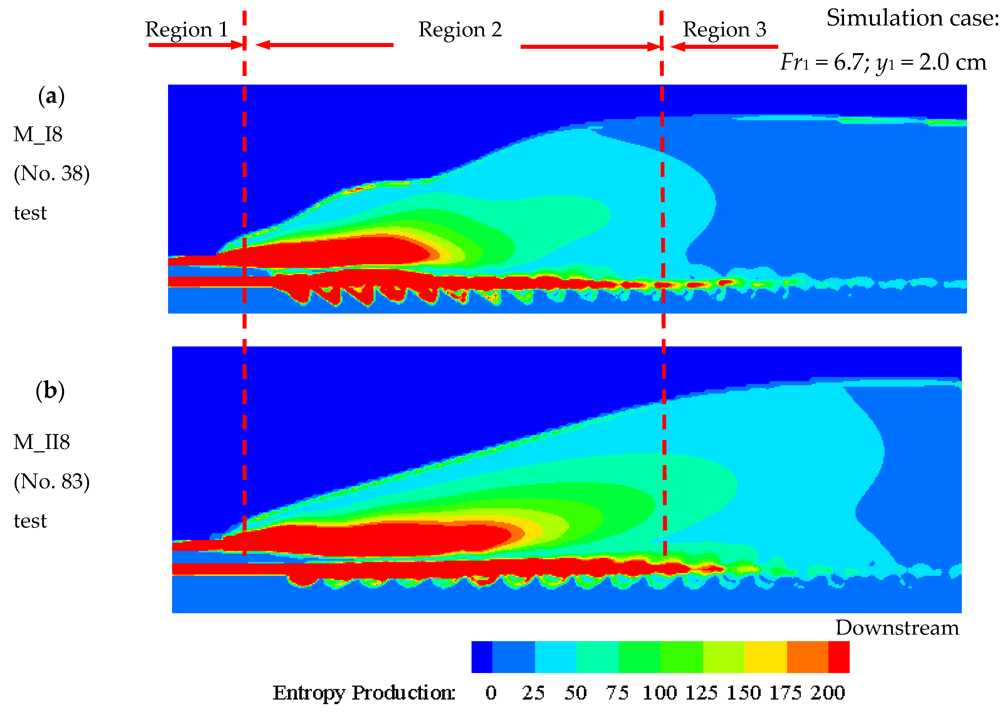
Recently, more and more researchers have reported that losses within internal flows often attributed to pressure losses are related to the local entropy production rate. The local energy dissipation rates could be figured out and integrated over the flow domain to obtain the losses. Therefore, to further clarify the influence of rough bed characteristics, in this section, we use the entropy production rate to analyze energy dissipation in hydraulic jumps. We used commercial software Tecplot (360 EX 2022R2 version 2022.2.0.18713) and the entropy determination formulas in Section 2.4 to display entropy distributions. Figure 21a,b shows the entropy production rate distribution in the case of the triangular rough bed with m1 = 0 (M_I8 (No. 38) test) and m2 = 0 (M_II8 (No. 83) test); for more detail see Table 7.

Figure 21.
Entropy production rate on the XZ-plane for two typical rough bed cases.
As per the picture presentation, the flow is divided into three regions: Region 1 is the upstream hydraulic jump’s beginning area; Region 2 is the hydraulic jump and Region 3 is the zone of stable flow after the hydraulic jump. The first region is the supercritical flow before the jump toe. There is a high entropy production region at the channel bottom surface, the incoming jet to the basin is fully developed, and the boundary layer is formed entirely in the incoming jet. The entropy production rate is higher because of the influence of the channel bottom. The second region is the hydraulic jump range. In this region, the flow suddenly changes from supercritical to subcritical, increasing water level depth downstream of the channel. The zone of the rough bed arrangement on the channel bottom, where the entropy production rate has a very high value of about 200 Wm−3K−1, was concentrated in the rough bed zone at about Lj/3, and then gradually decreased towards the downstream hydraulic jumps for the M_I8 model, No. 38 test (see Figure 21a). This region has a clear difference in entropy production distribution for the two cases of triangular prism elements. Figure 21a shows that the triangular prism elements have a shape that conflicts with the flow direction m1 = 0 (model No.38 test); the entropy production rate is higher near the jump toe and quickly tapers off after four to five rough rows.
Meanwhile, with the triangular rough elements having a shape in the flow direction m2 = 0 (model No.83 test), the entropy production still has a significant value but is distributed along the jump length. The figure shows the flow close to the bottom slips on the crest of the triangular rough elements. Thus, the triangular rough elements shaped m1 = 0, which conflicts with the flow direction, have a better energy dissipation effect than the flow direction shape. Therefore, the character shape of a rough bed has a significant effect on reducing hydraulic jump length.
The third region is the flow range behind hydraulic jumps. In this zone, the subcritical flow was formed. The entropy production is minimal (<30 Wm−3K−1), meaning the hydraulic jump had effective energy dissipation.
4. Conclusions
This research evaluated and investigated the effects of four right triangular prism rough bed types arranged in a channel bed (stilling basin) on hydraulic jumps. The considerable variation in boundary conditions, including supercritical flow conditions and geometry characteristics of the roughness elements, were provided by the initial Froude number (Fr1) from 4.8 to 9.4, the wave steepness values (t/s) of 0.67 ≤ t/s ≤ 1.33, and the relative distance of roughness elements of 0.0 ≤ Ls/y1 ≤ 4.0. The hydraulic jump characteristics, such as sequent depth, jump length, energy loss, and bed shear stress, primarily depended on Fr1. These hydraulic parameters increase with the increase in Fr1 and vice versa. Meanwhile, the rough bed models’ two main geometry parameters (t/y1 and Ls/y1) do not have much of an influence on directly reducing the sequent depth and jump length. However, they affect increased bed shear stress on the channel bottom and energy loss in flow.
This study indicated that the arrangement of the right triangular prism rough elements on the stilling basin increased bed shear stress from 6 to 17 times compared with a smooth bed, and the energy loss also increased from 6% to 24%. Therefore, the result leads to conjugate depth and jump length, which are about 22% and 50% shorter than on a smooth bed, respectively. The study results show that the effective jump length reduction is more significant with a high Froude number (Fr1).
Entropy production was used to demonstrate the energy dissipation in the hydraulic jump. The study results indicated that the energy dissipation was more substantial in the hydraulic jump zone. The triangular rough elements shaped with m1 = 0, which conflicts with the flow direction, have a better energy dissipation effect than in the flow direction shape (m2 = 0). Therefore, the character shape of a rough bed has a significant effect on reducing hydraulic jump length. The results indicated that arranging rough beds within the jump length region reduced the conjugate depth and jump length. The rough bottom area arranged after the hydraulic jump has a minimal influence on the energy dissipation of the flow; this may be because the downstream flow has changed into a subcritical flow with a small amount of energy. Therefore, it needs a suitable rough bed structure solution with a rough bed region of about 2Lj/3.
The results of this study indicate that these rough beds have a positive effect on hydraulic jumps, such as reduced conjugate depth and jump length. Therefore, this work recommends that right triangular prism rough bed models be used as an alternative method to control the location of free and steady hydraulic jumps for energy dissipation work. It is necessary to renovate the small and medium irrigation work types or urban sewer systems that do not have the stilling basin and use the classical jump under the impact of increasing flood discharge due to climate change.
Author Contributions
Writing—original draft, C.T.T. (Cong Ty Trinh), J.Z. and C.T.T. (Cong Trieu Tran). All authors have read and agreed to the published version of the manuscript.
Funding
This research received no external funding.
Institutional Review Board Statement
Not applicable.
Informed Consent Statement
Not applicable.
Data Availability Statement
The data presented in this study are available in article.
Conflicts of Interest
The authors declare no conflicts of interest.
References
- Ead, S.; Rajaratnam, N. Hydraulic jumps on corrugated beds. J. Hydraul. Eng. 2002, 128, 656–663. [Google Scholar] [CrossRef]
- Abbaspour, A.; Dalir, A.H.; Farsadizadeh, D.; Sadraddini, A.A. Effect of sinusoidal corrugated bed on hydraulic jump characteristics. J. Hydro-Environ. Res. 2009, 3, 109–117. [Google Scholar] [CrossRef]
- Abbaspour, A.; Farsadizadeh, D. Numerical study of hydraulic jumps on corrugated beds using turbulence models. Turk. J. Eng. Environ. Sci. 2009, 33, 61–72. [Google Scholar]
- Samadi-Boroujeni, H.; Ghazali, M.; Gorbani, B.; Nafchi, R.F. Effect of triangular corrugated beds on the hydraulic jump characteristics. Can. J. Civ. Eng. 2013, 40, 841–847. [Google Scholar] [CrossRef]
- Ghaderi, A.; Dasineh, M.; Aristodemo, F.; Ghahramanzadeh, A. Characteristics of free and submerged hydraulic jumps over different macroroughnesses. J. Hydroinformatics 2020, 22, 1554–1572. [Google Scholar] [CrossRef]
- Ghaderi, A.; Dasineh, M.; Aristodemo, F.; Aricò, C. Numerical simulations of the flow field of a submerged hydraulic jump over triangular macroroughnesses. Water 2021, 13, 674. [Google Scholar] [CrossRef]
- Tokyay, N.D. Effect of channel bed corrugations on hydraulic jumps. In Impacts of Global Climate Change; American Society of Civil Engineers: Reston, VA, USA, 2005; pp. 1–9. [Google Scholar]
- Izadjoo, F.; Shafai-Bejestan, M. Corrugated bed hydraulic jump stilling basin. J. Appl. Sci. 2007, 7, 1164–1169. [Google Scholar] [CrossRef]
- Jalil, S.A.J.; Sarhan, S.A.; Ali, S.M. Characteristics of hydraulic jump on a striped channel Bed. J. Duhok Univ. 2017, 20, 654–661. [Google Scholar]
- Dasineh, M.; Ghaderi, A.; Bagherzadeh, M.; Ahmadi, M.; Kuriqi, A. Prediction of hydraulic jumps on a triangular bed roughness using numerical modeling and soft computing methods. Mathematics 2021, 9, 3135. [Google Scholar] [CrossRef]
- Viti, N.; Valero, D.; Gualtieri, C. Numerical Simulation of Hydraulic Jumps. Part 2: Recent Results and Future Outlook. Water 2018, 11, 28. [Google Scholar] [CrossRef]
- Trieu, T.C.; Ty, T.C. Prediction of the Vortex Evolution and Influence Analysis of Rough Bed in a Hydraulic Jump with the Omega-Liutex Method. Teh. Vjesn.-Tech. Gaz. 2023, 30, 1761–1768. [Google Scholar]
- Nikmehr, S.; Aminpour, Y. Numerical Simulation of Hydraulic Jump over Rough Beds. Period. Polytech. Civ. Eng. 2020, 64, 396–407. [Google Scholar] [CrossRef]
- Ebrahimi, S.; Salmasi, F.; Abbaspour, A. Numerical study of hydraulic jump on rough beds stilling basins. J. Civ. Eng. Urban. 2013, 3, 19–24. [Google Scholar]
- Ghaderi, A.; Abbasi, S.; Abraham, J.; Azamathulla, H.M. Efficiency of trapezoidal labyrinth shaped stepped spillways. Flow Meas. Instrum. 2020, 72, 101711. [Google Scholar] [CrossRef]
- Yakhot, V.; Orszag, S.A.; Thangam, S.; Gatski, T.B.; Speziale, C.G. Development of turbulence models for shear flows by a double expansion technique. Phys. Fluids A Fluid Dyn. 1992, 4, 1510–1520. [Google Scholar] [CrossRef]
- Hirt, C.W.; Nichols, B.D. Volume of fluid (VOF) method for the dynamics of free boundaries. J. Comput. Phys. 1981, 39, 201–225. [Google Scholar] [CrossRef]
- Bejan, A. Entropy Generation through Heat and Fluid Flow; John Wiley: New York, NY, USA, 1994. [Google Scholar]
- Schmandt, B.; Herwig, H. Internal Flow Losses: A Fresh Look at Old Concepts. J. Fluids Eng. 2011, 133, 051201. [Google Scholar] [CrossRef]
- Kock, F.; Herwig, H. Entropy production calculation for turbulent shear flows and their implementation in CFD codes. Int. J. Heat Fluid Flow 2005, 26, 672–680. [Google Scholar] [CrossRef]
- Celik, I.B.; Ghia, U.; Roache, P.J.; Freitas, C.J. Procedure for estimation and reporting of uncertainty due to discretization in CFD applications. J. Fluids Eng.-Trans. ASME 2008, 130, 078001. [Google Scholar]
- Khan, A.A.; Steffler, P.M. Physically based hydraulic jump model for depth-averaged computations. J. Hydraul. Eng. 1996, 122, 540–548. [Google Scholar] [CrossRef]

Disclaimer/Publisher’s Note: The statements, opinions and data contained in all publications are solely those of the individual author(s) and contributor(s) and not of MDPI and/or the editor(s). MDPI and/or the editor(s) disclaim responsibility for any injury to people or property resulting from any ideas, methods, instructions or products referred to in the content. |
© 2024 by the authors. Licensee MDPI, Basel, Switzerland. This article is an open access article distributed under the terms and conditions of the Creative Commons Attribution (CC BY) license (https://creativecommons.org/licenses/by/4.0/).