Abstract
Brain complexity relies on the integrity of structural and functional brain networks, where specialized areas synergistically cooperate on a large scale. Local alterations within these areas can lead to widespread consequences, leading to a reduction in overall network complexity. Investigating the mechanisms governing this occurrence and exploring potential compensatory interventions is a pressing research focus. In this study, we employed a whole-brain in silico model to simulate the large-scale impact of local node alterations. These were assessed by network complexity metrics derived from both the model’s spontaneous activity (i.e., Lempel–Ziv complexity (LZc)) and its responses to simulated local perturbations (i.e., the Perturbational Complexity Index (PCI)). Compared to LZc, local node silencing of distinct brain regions induced large-scale alterations that were paralleled by a systematic drop of PCI. Specifically, while the intact model engaged in complex interactions closely resembling those obtained in empirical studies, it displayed reduced PCI values across all local manipulations. This approach also revealed the heterogeneous impact of different local manipulations on network alterations, emphasizing the importance of posterior hubs in sustaining brain complexity. This work marks an initial stride toward a comprehensive exploration of the mechanisms underlying the loss and recovery of brain complexity across different conditions.
1. Introduction
Over the years, the concept of brain complexity has gained traction within neuroscientific research. In this general framework, brain networks strike an optimal balance between the requirement for functional specialization (differentiation) and that for tight interactions (integration) across modules [1,2,3]. Within a continuum ranging from segregated subsystems to an entirely homogeneous macrosystem, the brain would fall in between, in a complex regime where functionally differentiated groups of neurons are able to engage in tight reciprocal interactions so that the whole is more than the sum of its parts [4,5].
Recently, this theoretical notion has drawn extensive empirical attention with several human and animal studies proposing empirical estimates of brain complexity [6]. Specifically, a growing body of experimental literature has demonstrated a reliable correlation between complexity measures and the presence or absence of consciousness across different conditions, confirming early theoretical principles [7].
Recently, structural human brain networks, also known as ‘connectomes’ [8,9], became available thanks to different initiatives like the Human Connectome Project and the UK Biobank Imaging project [10,11,12]. When such networks are endowed with mathematical models of local excitability in each node, they allow the development of computational models to simulate whole-brain dynamics [13,14,15]. These models provide a controlled and mechanistic framework to explore a broad spectrum of parameters that are potentially relevant for better understanding global brain properties such as those implicated in brain complexity [2,16].
Most empirical and computational investigations have explored network complexity based on spontaneous neural activity [6]. Such an observational approach can be usefully complemented by a causal approach, whereby stimulations are used to assess the complexity of neuronal interactions from a causal, rather than correlational, perspective. Along these lines, the Perturbational Complexity Index (PCI) [17] empirically estimates the joint presence of differentiation and integration by quantifying the richness of the spatiotemporal patterns of cortical activity extracted from the electroencephalographic (EEG) response to a brief local perturbation with transcranial magnetic stimulation (TMS). PCI has provided a reliable index to assess the loss and recovery of consciousness in both physiological and pathological conditions [18]. Supported by a series of multiscale experiments in cell cultures [19,20], cortical slices [21], animal models [22,23,24], and intracranial and extracranial human studies [17,18,25,26,27,28,29], this perturb-and-measure approach has also recently been applied in silico. This computational neuroscience implementation can further elucidate the mechanistic link between brain complexity and anatomic-physiological brain properties. Specifically, the relationship between brain complexity and structural connectivity [30,31] as well as functional network properties [32] have been investigated. In addition, the modulations of brain complexity dependent on global neuromodulation [33] as well as local node properties [34] have been recently addressed.
Crucially, it is also possible to link single node properties to large-scale network dynamics [35,36] and explore the global effects of local manipulations, such as virtual lesions [37] and silencing [38].
Previous computational investigations have shown that large-scale spontaneous network dynamics change considerably upon local connectivity alterations (i.e., local node deletion within spatially defined regions) [39]. Along these lines, a strong reduction of brain-wide activity was observed particularly when simulating the regional inactivation of posterior areas [40]. These results are particularly relevant in view of a postulated critical role of posterior regions of the cortex [41,42] in supporting complexity and consciousness. So far, however, computational studies relating local properties to global brain states have focused mostly on spontaneous activity [37] and have not explored the complexity of neuronal interaction from a causal perspective (i.e., using controlled model perturbations).
Here, we exploited direct perturbations and investigated the large-scale impact of controlled local manipulations (i.e., local node silencing) on network activity and brain complexity in a whole-brain computational model. Specifically, using “The Virtual Brain” platform [13,43], we extensively and systematically varied the topology of the stimulated and the silenced nodes and performed a direct comparison between metrics derived from observational (Lempel–Ziv complexity) [44] and perturbational approaches (PCI). In addition, we explored critical properties governing the network information flow [45] and linked specific features of network organization (i.e., integration and segregation) to the above-mentioned network complexity metrics.
Our intact model exhibited complex spontaneous patterns emerging from the structural links of the connectome and engaged in complex and enduring cortical interactions following focal exogenous perturbations closely resembling the empirical TMS-EEG responses. Importantly, node manipulations revealed an overall reduction of network complexity measures, underlining interesting dissociations between observational and perturbational metrics. Interestingly, the impact of local manipulations was highly heterogeneous, and the comprehensive spatial sampling of the implemented node silencing allowed assessing relevant regional aspects with respect to the role of posterior cortical regions for brain complexity.
Overall, our results aim at better characterizing the effects of local manipulations on large-scale network dynamics and may serve as a useful tool to systematically assess the mechanisms underlying the loss and recovery of brain complexity in pathological conditions.
2. Materials and Methods
2.1. Model Simulations
2.1.1. Structural Connectivity
For the main results of this study, we employed a connectome composed of 76 areas available in the TVB simulator (2.7.2) (named “Default” connectome, Dconn). Dconn is based on an anatomical tracing reconstruction (CoCoMac) [46] with directional connections and is therefore well suited to investigate propagating activities in brain networks [47]. Additionally, we implemented a subset of analyses on a connectome with finer parcellation consisting of 998 areas (named “Hagmann” connectome, Hconn [48]), as described in Section 2.1.5.
2.1.2. Neural Mass Model
To model the mesoscopic dynamics of cortical regions, we used the Larter and Breakspear model [49], a conductance-based neural mass model widely employed for simulating whole-brain dynamics in intact networks [50,51,52,53,54,55,56,57,58] and lesioned networks [39,59]. According to the model, the dynamics of a node k are governed by the following ordinary differential equations (ODEs):
where V is the mean membrane potential of the excitatory pyramidal neurons, Z is the mean membrane potential of the inhibitory interneurons, and W is the average number of open potassium ion channels. The term rNMDA is the ratio of NMDA receptors to AMPA receptors, and axy is the synaptic strength originating from population x (e.g., e, i, n, where e refers to the excitatory population, i to the inhibitory one, and n denotes a nonspecific input) to population y (e.g., e, i). The rate terms b and ϕ govern the time scales of Z and W, respectively. The term gion is the maximum conductance (i.e., when all channels are open) of the corresponding ion species. The voltage-dependent fractions of open channels for a given ion is determined by mion and is modeled by a sigmoidal shape function:
where Tion is the mean threshold membrane potential of a given ion channel population, and δion is its standard deviation. The mean firing rates of the excitatory and inhibitory populations are determined by the voltage-dependent activation functions QV and QZ, respectively, modeled as:
where QVmax and QZmax are the maximum firing rates of the excitatory and inhibitory populations, respectively. Their corresponding thresholds for action potential generation are given by the terms VT and ZT, with standard deviations δV and δZ, respectively. The network input to node k is given by:
where ukj is the connection weight from node j to node k, τ is the input delay time, and G is the global coupling that scales the connection weights. The parameter C in Equation (1) ranges within [0, 1] and balances the strength of the self-connections against those of the rest of the network.
The ODEs were solved starting from random initial conditions with the stochastic Heun integration method available in TVB (with additive Gaussian noise, standard deviation SD = 10−7) and an integration time step of 0.1 ms. A pre-processing step was performed to reduce the amount of data by temporally resampling the data to a resolution time of 1 ms (i.e., averaging over each 1 ms time step). In addition, the first 3 s of simulations were discarded (first 14 s in Hconn) to remove the initial transient activities in the model.
In order to improve the responsiveness of the nodes (e.g., propagating activities) to stimulation, we varied a set of parameters (indicated in bold in Table S2) with respect to other studies that investigated only the model’s spontaneous activity (e.g., [39]). In addition, we set the global coupling G (Equation (7)) in such a way as to maximize the overlap between the functional and the structural connectivity (Figure 1c, see also [60]).
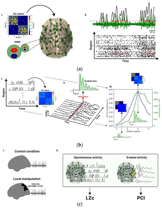
Figure 1.
Whole-brain model for investigating brain complexity in silico. (aI) Each node of the whole-brain network is modelled by the Larter and Breakspear (LB) neural mass model (NMM), describing the interaction between excitatory (E) and inhibitory (I) neurons. The weights connecting the nodes are reported in the structural connectivity (SC) matrix. (aII) The output of the model of a given node is the mean membrane potential of the excitatory population (green trace), and the timing of the spikes (red dots), detected with a hard threshold on the voltage, are then converted to an instantaneous firing rate (IFR) (black overlay trace). (b) The working point of the model (i.e., set of model parameters) was obtained based on the spontaneous and evoked activity following three steps. First (bI), the correlations between the spontaneous IFR traces were computed to estimate a functional connectivity (FC) matrix. Then, the similarity between the FC and SC matrices was assessed through the Pearson correlation coefficient. Second (bII), by stimulating a node of the connectome (here rPCi), the propagation of activity in the network was quantified in terms of ΔIFRSH (ΔIFR averaged over the nodes of the stimulated hemisphere), and some representative trials of ΔIFRSH are reported. The evoked area is obtained as the integral after stimulation (red line, between 0 and 500 ms) of ΔIFRSH averaged across trials. Third (bIII), the SC-FC correlation and the evoked area are reported for different global couplings (i.e., a scaling factor of the SC), and both metrics reached a peak at G = 4 (working point). The dashed blue lines and arrows illustrate the matches between the FC and the SC maps for different G values. The dashed green lines and arrows illustrate the evoked area by the stimulus. (cI) We simulated control and local manipulation conditions. Local manipulations were implemented by silencing selected nodes. (cII) To assess the impact of local node silencing on spontaneous complexity, we calculated Lempel–Ziv complexity (LZc) on ongoing network activity. Furthermore, we separately stimulated different connectome nodes under different local manipulations and calculated the Perturbational Complexity Index (PCI) to gauge the impact of local silencing on the evoked activity.
2.1.3. Spontaneous Activity and Stimulation Protocol
For the analysis of spontaneous activity, each condition was run for 4000 s, and the time-series were split into 10 segments of 400 s.
On the other hand, to examine the model’s evoked response, a square wave pulse of 5 ms and amplitude 1 was applied to a single connectome node, specifically targeting the excitatory pyramidal cells (as an additive term to Equation (1)). In our study, we individually stimulated a total of 12 nodes located in the right hemisphere (see Section 2.1.4 below for details), homogeneously sampling all cortical lobes (Table 1).

Table 1.
Labels of the cortical nodes and their description in Dconn. The stimulated nodes are reported in bold.
In all conditions (control and lesions) a stimulus was delivered to the same node (i.e., same stimulus) 500 times (500 trials) by reinitializing each simulation. We also jittered the onset of the stimulus within a range of 2 s. Note that in the Larter–Breakspear model, all quantities are dimensionless except for time [56], which allows a straight comparison with the experimental time courses.
2.1.4. Local Manipulation Modeling
Building upon prior modeling studies [38,40,61], we simulated local network alterations by reducing the excitability of selected nodes. This silencing was achieved by hyperpolarizing the manipulated nodes (Figure 1c) to an extent which completely suppresses their firing activity (mean firing rate = 0). To achieve this, we abolished the excitatory nonspecific input (ane = 0) and increased the nonspecific inhibitory input (ani = 0.6). We implemented the different manipulations in one hemisphere (the right hemisphere) to simulate an affected hemisphere and an intact one (left hemisphere). Consistent with empirical studies [27], we stimulated the affected hemisphere to assess cortical reactivity following perturbation near the silenced node.
In line with previous work where 5% of the nodes were lesioned [39], in our study each manipulation involved approximately 4% of the connectome nodes (three nodes). As in [39], each local manipulation was defined by first choosing a central node (center of the manipulation) to be silenced and then selecting the remaining nodes to silence based on a geometrical distance criterion (Euclidean distance) from the central node. Manipulation details are reported in Table 2. Whenever the stimulated and manipulated nodes overlap, the latter were replaced with the closest non-manipulated nodes to the center of the manipulation. For instance, when stimulating rPCip, which was also part of local manipulation 1 (L1), we spared rPCip and silenced the next closest node (rV2). For a fair comparison across conditions between spontaneous and evoked metrics, non-identical manipulations were excluded whenever a correlation was performed (e.g., in Table S4 in Supplementary Material).
Table 2.
Local manipulation labels in the Dconn connectome. The labels of the local manipulations and the corresponding nodes silenced in the Dconn connectome. The ranking is based on the MFR difference (from lowest to highest). Note that when a stimulus overlaps with a silenced node (in bold), the latter is replaced by a nearby node.
This procedure resulted in a total of 12 control conditions (stimulations without any node manipulation) and 240 manipulation conditions (silencing of 20 different nodes for each stimulation, 12 × 20).
2.1.5. Validation on a Larger Connectome (Hconn)
As a proof of concept aimed at confirming the validity of the observed findings, we repeated the analysis pertaining to PCI using a connectome endowed with finer parcellation (Hconn) consisting of 998 areas [48]. Hconn corresponds to a human connectome, with symmetric bidirectional connections, and has been used in several studies [39,51,56,62]. We tested a control condition and 20 local node manipulations, which are detailed in Table S3 (Supplementary Material). Each of them involved approximately 4% of the nodes (40 nodes), and the implementation procedure was the same as in Section 2.1.4 (with the only exception being that in Dconn, ani = 0.6, while in Hconn, ani = 0.65, as more inhibition was required to suppress firing activity). In Hconn, we limited the number of stimulations to one performed over a portion of the superior parietal cortex (SP, Table S1 in Supplementary Material) of the manipulated hemisphere. In particular, to maintain a comparable fraction of stimulated nodes with the Dconn connectome (1/76 = 0.013), a total of 14 nodes of SP were simultaneously stimulated (14/998 = 0.014) that were chosen based on their adjacency to a central node, following the same geometrical approach used in Section 2.1.4. As in Dconn, the stimulus was delivered 500 times (500 trials) in each condition (see Section 2.1.3).
2.2. Analysis of Network Simulations
2.2.1. Firing Activity Analysis
The first step of all analysis consisted in the detection of spiking activity of all nodes of the network. Spike timing was established as the passage of membrane potential of the nodes above a fixed threshold (−0.05, Figure 1a).
We defined the mean firing rate for each region/node of interest (MFRROI) as the amount of spikes divided by the time window of observation.
To characterize the global/population activity of the model (MFR), we averaged the MFRROI values across nodes (either all nodes or, when specified, the ones of the intact or the manipulated hemisphere):
Then, to quantify the impact of the local manipulation on activity, we defined the MFR difference (MFRΔ) as:
where MFR(condition) refers to the MFR in a condition of interest. Note that the MFRΔ involved only the nodes not affected by the local manipulation (i.e., excluding the silenced nodes also in the control condition).
Then, for each node we defined the time-dependent Instantaneous Firing Rate (IFR(t), in Hz) as the frequency of spikes in a time window of 25 ms, and the temporal dependence was obtained by sliding the time window by 10 ms on the simulated data. We varied the size of the time window (e.g., 50 ms) and found qualitatively similar results.
In order to quantify the impact of the stimulation on the node’s activity, we defined the quantities:
where <IFR(t, trial)>(t<0) is the average IFR over the time prior to stimulation, and <ΔIFR(t)>trials is the average ΔIFR across trials.
The level of network synchrony was quantified through the averaged pairwise cross-correlation between the spontaneous IFR signals:
where <…> denotes the average over all possible pairs of nodes (excluding silenced nodes), Cov(IFRi, IFRj) is the covariance between two spontaneous IFR signals (IFRi, IFRj), and σ(IFRi), σ(IFRj) are the corresponding standard deviations of the IFR signals
2.2.2. Network Analysis
We employed graph metrics based on the weighted degree to assess the centrality of a node in the network [63]. In the Dconn connectome, we computed the weighted out-degree (WD) of each node (sum of weighted outgoing connections of a node) in order to analyze the relationship between network centrality and complexity index topographies (see below, Section 2.2.3 and Section 2.2.4). Notice that in symmetrical graphs, such as Hconn and non-directional functional connectivity (see below), the out-degree of a node is equal to its in-degree.
We computed the same quantities on the spontaneous functional connectivity (FC) in the control condition. The strengths of the functional connections between node pairs were obtained as the pairwise Pearson’s correlation coefficient between their spontaneous instantaneous firing rates (IFRs). In addition, to corroborate our findings, we computed the FCBOLD on the BOLD signal, a widely used approach in the literature with this model [39,50,51,56,57,58]. The BOLD signal was estimated from the model’s output following [39]. We used the nonlinear Balloon–Windkessel hemodynamic model [64], and the input to the model was the absolute value of the time derivative of the excitatory membrane potential within each node. All the hemodynamic parameters were taken from [64]. Lastly, the estimated BOLD signal was sampled every 2 s. The FCBOLD is defined as the Pearson correlation coefficient between each pair of BOLD signals. Then, similar to the SC analysis, we used the WD from the FCIFR and the FCBOLD to investigate the relationship between node centrality and complexity topographies. We also conducted the analysis by performing global signal regression (GSR) on the BOLD signal [51].
2.2.3. Complexity Indices
- -
- Lempel–Ziv Complexity
The spatiotemporal differentiation of the spontaneous instantaneous firing rate was calculated by the Lempel–Ziv complexity (LZc) [44]. The optimal time window to compute LZc was examined by selecting temporal segments of variable lengths (from 1 s to 800 s). LZc decreased when increasing the temporal segments and reached a plateau around 200 s, and starting from 400 s, the variability, quantified by the coefficient of variation (CV), was less than 0.0004. For each condition, we calculated LZc over 10 segments of spontaneous activity (400 s each) and reported its mean ± SD.
- -
- Perturbational Complexity Index
The Perturbational Complexity Index (PCI) quantifies the spatiotemporal complexity of brain activity evoked by an external perturbation [17]. To compute PCI, we followed the procedure outlined in [17], with the notable difference that we applied it to the IFR time series of the brain nodes.
In short, the significant evoked activities of each node, with respect to baseline, were determined by applying a non-parametric permutation test to the IFR. The baseline activity (pre-stimulus, time window = [−1000, 0 ms]) was used to determine, for each node, thresholds of significance (significance level set to 0.01, 500 bootstraps) and accounting for multiple comparison testing using the maximum test statistic. In this way, we derived a spatiotemporal matrix of significant activity [SS(x,t)], where SS(x,t) = 1 for significant activity in node x at time t, and SS(x,t) = 0 otherwise. The SS matrix was then sorted according to the amount of significant activity during the post-stimulus interval of each node (e.g., most/less active at the bottom/top rows). Then, the Lempel–Ziv complexity (CL) was calculated on the binary matrix [SS(x,t)] of the significant IFR (first 500 ms after the pulse).
Finally, PCILZ is defined as the normalized CL of the evoked spatiotemporal patterns SS(x,t):
where L is the size of the matrix [SS(x,t)] (L = number of nodes × number of time samples), and Hsrc is the source entropy given by:
where p1 and (1 − p1) are the fraction of “1” (significant activity) and “0” (non-significant activity) in the binary matrix.
Spatial temporal maps were represented based on SS and the <ΔIFR(t)> (Equation (10)). In particular, for each time point t, the ΔIFR(t) of the nodes with significant activity (i.e., SS(., t) = 1) were reported.
In all conditions (control and manipulations), each stimulus was repeated 500 times. Then, 10 resamples of 300 trials (without repetitions) were formed, and the PCI was computed on each subgroup. We assessed the stability of PCI versus the number of trials (ranging from 10 to 500 trials) and observed that the PCI values reached a plateau around 200 trials, and starting from 300 trials, the variability (CV) was less than 0.01.
2.2.4. Complexity Topographies
The contribution of each node to the complexity indices used was investigated by performing linear regressions between the complexity values (LZc and PCI) and the spontaneous activity of each node (MFRROI) for different conditions (local manipulations and control). The coefficient of determination (R2) for each node was then computed and mapped onto the brain topographies. Thus, LZc-R2 and PCI-R2 topographies were derived. Given the 12 stimulation sites for PCI, 12 topographies were generated, which were then averaged into a single PCI-<R2> topography.
2.2.5. Statistical Analysis
Statistical analyses were performed using Python 3.7, employing the SciPy (1.9.3), statsmodels (0.13.5), and scikit-posthocs (0.8.1) packages. The data are expressed as mean ± standard deviation (SD) unless otherwise indicated. The boxplots report the first and third quartiles (lower/upper line of the box), the mean of the distribution (horizontal line in the box), and the whiskers (5th and 95th percentiles). The data were checked for normal distribution and homogeneity of variance using Shapiro–Wilk test and Levene test, respectively. According to the results, either parametric (e.g., one-way ANOVA and t-test) or non-parametric (e.g., Kruskal–Wallis H-test and Dunn’s test) tests were performed. p values were adjusted for multiple comparisons using the Benjamini–Hochberg method to control the false discovery rate. Multiple one-sample t-tests were conducted with Bonferroni–Holm p-values correction to test the impact of each local manipulation compared with the control. Linear correlation between the metrics was computed with the Pearson correlation coefficient and its associated two-sided p-value. We conducted simple and multivariate linear regressions, calculating the coefficient of determination (R2, and R2adjusted to account for multiple regressors) and the p-value of the F-statistic. Additionally, we computed the slope coefficients of the regressors and their corresponding two-sided 95% confidence intervals (95% CI). For all statistical analyses, alpha = 0.05.
3. Results
3.1. Spontaneous Activity
Impact of Local Node Silencing on Spontaneous Complexity Measures
We first investigated the impact of local silencing on the model’s spontaneous activity by quantifying the mean firing rate difference (MFRΔ) on the nodes within the manipulated hemisphere, the intact one, as well as in the entire model compared with the same nodes in the control condition (Figure 2a). This analysis revealed that the MFR decreased the most in the affected hemisphere (MFRΔ = −3.621 ± 1.629 Hz, mean across all manipulations ± SD) and to a lesser extent in the intact hemisphere (−1.431 ± 0.992 Hz).
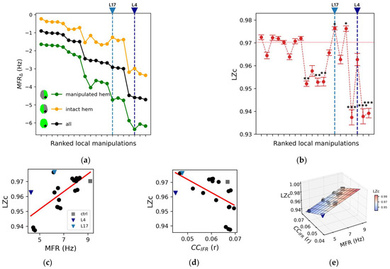
Figure 2.
Impact of local manipulations on whole-brain spontaneous activity. (a) Mean firing rate difference (MFRΔ, see Methods) for each silencing condition of the manipulated hemisphere (green), the intact one (yellow), and overall nodes (black). Note that the ranking (i.e., ranked local manipulations, see Table 2) is based on the black curve. (b) The Lempel–Ziv complexity (LZc) metric is reported versus the same ranked local manipulations. The red horizontal lines mark the average value of LZc in the control condition. Error bars represent one standard deviation and asterisks indicate a statistically significant difference from the control condition (* p < 0.05, ** p < 0.01, *** p < 0.001; Kruskal–Wallis and Dunn post hoc test with Benjamini–Hochberg correction). (c) Linear regressions relating the mean firing rate of all nodes (MFR) to LZc (r = 0.69; p = 0.0005). (d) Linear regression relating the averaged pairwise cross-correlation (CCIFR) to LZc (r = −0.55, p = 0.009). (e) Multivariate regression of LZc with respect to the independent variables MFR and CCIFR (R2 = 0.98, R2adjusted = 0.98, p = 2 × 10⁻¹⁶).
We then quantified the impact of local node silencing on the complexity of spontaneous brain dynamics by computing Lempel–Ziv complexity (LZc) on the instantaneous firing rate (IFR) derived from the model time-series (Figure 2b). Notably, in 12 out of 20 local manipulations, LZc was not statistically different from control (Kruskal–Wallis and Dunn post hoc test with Benjamini–Hochberg correction). As a consequence, even though LZc positively correlated with MFR (LZc: r = 0.69; p = 0.0005, Figure 2c), it did not reflect the changes of network complexity with respect to control condition.
Further exploring the network properties relevant for complexity, we computed the averaged pairwise cross-correlation (CCIFR, see methods) between nodes as a measure of the synchrony of network interactions. CCIFR was lower across local manipulations when compared to control (control: 0.067, average across manipulations: 0.061 ± 0.007; Figure 2d), which corresponds to a larger segregation of the network patterns. We found a negative correlation between LZc and CCIFR (r = −0.55, p = 0.009; Figure 2d).
Considering the combined role of brain activity levels (MFR) and network interactions (CCIFR) in shaping brain complexity, we performed a multivariate regression between MFR and CCIFR in explaining LZc across all conditions (Figure 2e). This model effectively captured the variance of LZc (R2 = 0.98, R2adjusted = 0.98, p = 2 × 10⁻¹⁶). Confirming the results obtained with the univariate analyses, a positive relationship was found for LZc with respect to MFR (slope coefficient, βMFR = 0.0072, 95% CI [0.0066, 0.0078]), while CCIFR was found to be negatively correlated with LZc (βCC = −1.2, 95% CI [−1.3, −1.1]).
3.2. Evoked Activity
3.2.1. Local Node Silencing and PCI
We performed an extensive investigation of the responses to different stimuli for different node silencing within the connectome (12 stimuli × 20 manipulations). The impact of local node silencing on stimulus-evoked spatiotemporal activity was quantified by the Perturbational Complexity Index (PCI).
All manipulations caused a decrease of PCI with respect to the control condition (PCIΔ) across stimuli (for each local manipulation p < 0.01, one sample t-test with Bonferroni–Holm correction; Figure 3a), albeit with a great variability depending on the specific stimulus-silencing pair (individual PCI values and statistical comparisons with respect to the control condition are reported in Figure S2).
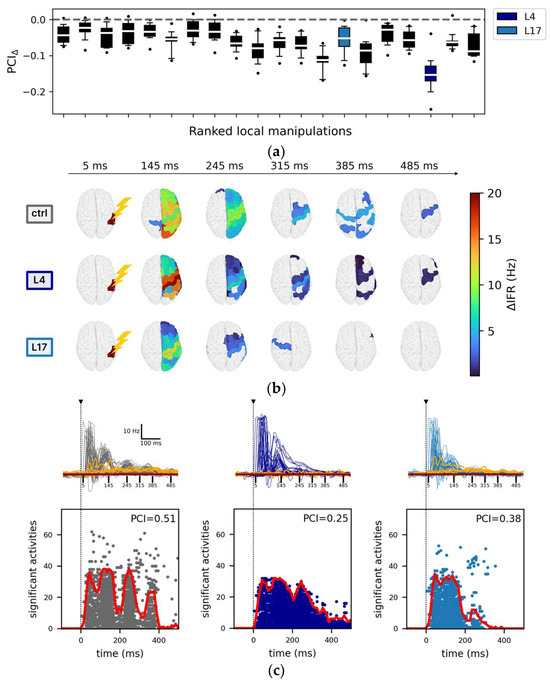
Figure 3.
Impact of local manipulations on evoked activity. (a) Each box, corresponding to a local manipulation (ordered according to the ranking in Figure 2), displays the difference in PCI compared to the control (PCIΔ) for a given stimulation site (12 values per box, e.g., stimulation of rPCi: PCIΔ (local manipulation) = <PCIlocal manipulation> − <PCIctrl>, where <…> indicates mean across resamples). For each local manipulation, p < 0.01 (one sample t-test against mean zero with Bonferroni–Holm correction). (b) Spatiotemporal distribution of the areas with significant changes of their firing rate with respect to baseline activity following stimulation. Representative snapshots are reported at time t = 5 ms, t = 145 ms, t = 245 ms, t = 285 ms, t = 375 ms, and t = 485 ms in the control condition (top row), for the local manipulations L4 (middle row), and L17 (bottom row). (c) Top: the temporal courses of the instantaneous firing rate (<ΔIFR>) are reported for all nodes and separately for the representative conditions: ctrl (grey), L4 (dark blue), and L17 (light blue). For each condition, the highest five <ΔIFR> (quantified as the total activity in the interval [0, 500] ms) of the non-stimulated hemisphere (orange traces) are also reported. The horizontal brown line indicates the mean baseline (defined as <ΔIFR(t)> averaged over the interval [−1000, 0] ms and over the latter highest five <ΔIFR(t)>). The vertical dotted black line marks the time of the stimulus, and the vertical continuous black lines are relative to the snapshots reported in panel b. Bottom: the corresponding sorted binary spatiotemporal matrices of significant activities highlight the impact of the local manipulations with respect to the control condition (the red line is the sum of significant activity over time). The Perturbational Complexity Index (PCI) decreases significantly (p < 0.00001, ANOVA and post hoc pairwise T test with Benjamini–Hochberg correction) in L4 and L17 compared with control (see Figure S2).
In this respect, the responses of the model to stimulation of the right inferior parietal cortex (rPCi) for the control and two highly segregated local manipulations (L4 and L17, see Table 2 for a description of the manipulated nodes) serve as an illustrative example of such variability.
Specifically, the spatiotemporal distribution of the significant activities (see Methods) elicited by the stimulation pulse in the control and in the two representative manipulations displayed marked differences (Figure 3b). In particular, compared to the control condition, in the case of L4 silencing, the response was sustained in time but spatially redundant (i.e., the significant activities often involved the same areas), and it did not involve the non-stimulated hemisphere as confirmed by the <ΔIFR> temporal profile (Figure 3c top panel). On the other hand, in the case L17 silencing, significant evoked activity extended to the non-stimulated hemisphere (Figure 3c top panel) but was short-lived. The richness of the significant spatial-temporal patterns evoked by a stimulus can also be described by the SS matrices (see Methods, Figure 3c bottom panels). Compared to the control condition, the SS matrix of both L4 and L17 were either restricted in space (i.e., evoked activity remained more local, as in L4) or in time (i.e., the significant evoked activity decayed rapidly, as in L17). Interestingly, in L4, the significant activity described by the source entropy (Hsrc) was comparable to the control (0.79 ± 0.03 and 0.79 ± 0.02, respectively), but the evoked activity was more redundant in time (compare Figure 3a), confirming the dissociations between PCI and Hsrc (Supplementary Results, Section S2, Figure S3) also found in empirical studies [17]. Consistent with these observations, we found a significant reduction of PCI (p < 0.00001, ANOVA and post hoc pairwise T t-test with Benjamini–Hochberg correction) for both L4 and L17 (Figure S2, grey arrows. Control: 0.49 ± 0.03; L4: 0.25 ± 0.01; L17: 0.37 ± 0.04).
Furthermore, to corroborate our results, we performed a similar analysis with the more detailed connectome, Hconn (Figure S4A,B). Again, we found a significant reduction of PCI (Figure S4C) in all manipulation conditions (for each p < 0.000001, ANOVA and post hoc pairwise T t-test with Benjamini–Hochberg correction). The higher reduction of PCI with Hconn compared to Dconn is likely due to a larger impact of node silencing on the local connectivity (i.e., areas surrounding the manipulation) as well as on the long-range connections reducing the communication between areas that are far apart.
3.2.2. The Impact of Regional Silencing on PCI
By taking advantage of the systematic and extensive investigation of stimulation/silencing pairs, we further explored the variability of the impact of local silencing on both spontaneous and evoked metrics and investigated the contribution of individual region activity (i.e., MFR) to PCI across all conditions. Thus, for each stimulation, we performed a linear regression of the PCI values (i.e., mean across resamples) versus the spontaneous mean firing rate of a node/region of interest (MFRROI) across all conditions (including the control condition and all local manipulations). Figure 4a shows the linear regressions for two representative ROIs (right posterior cingulate cortex; rCCp and right parahippocampal cortex; rPHC), corresponding to the ROIs showing the third highest and third lowest average correlations across stimuli, respectively. For each of the two ROIs, we show two representative stimulations delivered to the inferior parietal cortex (PCi; R2 = 0.59, p = 5 × 10⁻⁵ and R2 = 0.02, p = 0.58) and the dorsolateral prefrontal cortex (PFCdl; R2 = 0.23, p = 0.03 and R2 = 0.01, p = 0.60). We found that PCI correlated well with MFRROI (CCp) for most stimulations (F-statistic of R2, 11 with p < 0.05, one with p = 0.051), ranging from 0.19 to 0.59 (0.41 ± 0.14) (Figure 4b). On the other hand, MFRROI (PHC) was always non-significantly correlated with PCI across the 12 stimulations (p > 0.05).
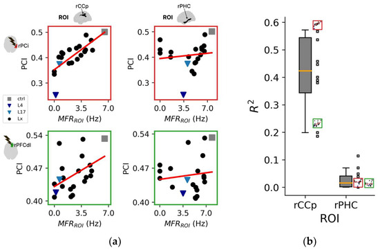
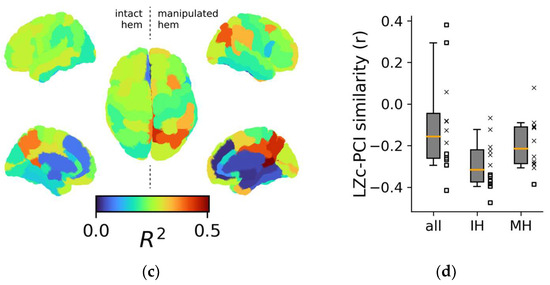
Figure 4.
Topological aspects of perturbational complexity. (a) Linear regressions relating PCI to the spontaneous mean firing rate of the ROIs/nodes rCCp and rPHC for two representative stimulation sites (red boxes: rPCi; green boxes: rPFCdl). (b) Boxplot of the R2 relative to the PCI versus MFRROI (rCCp) and PCI versus MFRROI (rPHC) linear regressions for all stimulation sites. Note that the reduced plots of panel A are reported on the right of the boxplot to highlight the corresponding R2 value. (c) Brain topography of the average R2 across stimulation sites (<R2>). For each ROI in the topography, the corresponding <R2> is derived as in panel (b). (d) Distributions of the Pearson correlation coefficients computed across the R2 topography maps of LZc with PCI and separately for all ROIs (all), intact hemisphere ROIs (IH), and manipulated hemisphere ROIs (MH). Each square and X symbol is relative to a stimulation site, and X markers indicate nonsignificant p values (>0.05).
The 12 regional maps of R2 coefficients for each stimulation are presented topographically in Figure S5A, and the average topography across all stimulations is presented in Figure 4c. Interestingly, the three ROIs with the highest average R2 across stimulations (i.e., CCr, <R2> = 0.51 ± 0.13; PCm, <R2> = 0.45 ± 0.14; CCp, <R2> = 0.41 ± 0.14) were located in the posterior cortex of the manipulated hemisphere. In addition, the ROIs with the three highest R2 values across all stimulations were predominantly located in the posterior regions (~89%, Figure S5B,C).
Consistently, we repeated the same analysis for the single stimulation on Hconn and found a similar regional specificity, with the highest R2 values located in posterior regions of the manipulated hemisphere (Figure S4D).
3.2.3. Assessing Regional Similarity between Spontaneous and Evoked Complexity Metrics
We performed separate linear regressions for MFRROI versus LZc (Figure S6A,B) and computed the similarity between the R2 topography maps of these and the 12 R2 PCI topographies for each stimulation (Figure 4d). We found that the correlations between PCI and LZ topographies were anti-correlated (−0.1 ± 0.23), though many correlations were not significant (5 out of 12). Similar results were obtained when restricting the analysis to either the intact or the manipulated hemisphere (−0.29 ± 0.11 and −0.19 ± 0.12, respectively).
3.3. Assessing the Relationship between Complexity Measures and Graph Properties
We explored the relationship between the R2-topographies derived from spontaneous (LZc) as well as perturbational complexity (PCI) measures and basic graph properties. To this aim, we correlated the weighted degree (WD) of each node (an index of network centrality calculated both on SC and FC) with the corresponding values of the complexity-R2 topographies (Figure 5). The WD computed on the SC showed a weak, albeit significant, correlation with the PCI average-R2 topography across the 12 stimulations (r = 0.34, p = 0.0026; Figure 5a). Conversely, we did not find a significant correlation with the LZc-R2 topography (p = 0.063, Figure 5b). Similarly, we found a significant correlation between the WD computed on the SC and the PCI-R2 topography applied to Hconn (r = 0.44, p = 2∙10−49; Figure S7A). Further, we found even more robust correlations between WD calculated on FC and the average PCI-R2 topography (r = 0.6, p = 10−8, Figure 5c). Again, no significant relationship was found between WD and the LZc-R2 topography (p = 0.5, Figure 5d). Similar results (Figure S7B–E) were obtained when using WD calculated on the FC derived from BOLD signals (FCBOLD; see Section 2).
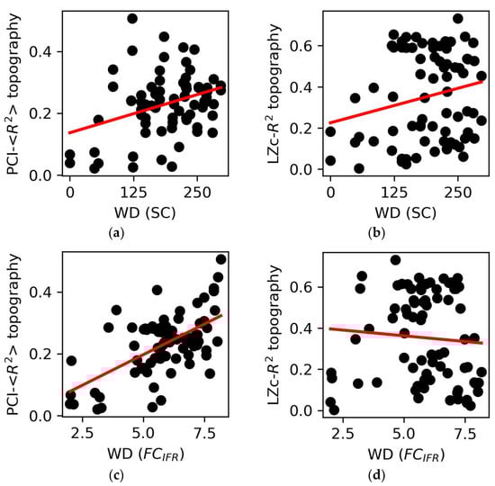
Figure 5.
Graph properties and complexity topographies. (a) The weighted degree (WD) of structural connectivity (SC) nodes correlated with the PCI-<R2> topography (r = 0.34, p = 0.0026) but (b) not with the LZc-R2 topography (p = 0.063). (c) The WD of the nodes of the functional connectivity (FCIFR) correlated with the PCI- <R2> topography (r = 0.6, p = 10−8) but (d) not with the LZc-R2 topography (p = 0.5). Each point is representative of an ROI/node in the network. The regression lines are reported in red.
4. Discussion
The present study employed whole-brain computer simulations, systematic local manipulations (i.e., node silencing), and perturbations (i.e., brief pulses applied to local nodes) to assess the circuit-level properties underlying estimates of brain complexity. Our model has proved to be particularly suitable for investigating the mechanisms underlying brain complexity using various metrics commonly employed in empirical studies. In the present implementation, we were able to obtain spontaneous network activity as well as complex and enduring cortical interactions upon exogenous perturbations (Figure 1b), reminiscent of empirical observations [17,36]. Unlike in previous simulation works [33] and in line with experimental data, in the present model, brief local pulses were effective in evoking responses that propagated across distant nodes while spanning more prolonged time intervals. The presence of the non-linear NMDA current as implemented in the Larter and Breakspear model [49] likely explains this important difference. Additionally, the same model has been shown to exhibit complex wave patterns, including traveling waves during spontaneous activity [56], thus arguably making it suitable for investigating complexity metrics that rely on activity propagation evoked by an external stimulus.
4.1. Impact of Local Silencing on Complexity Measures: The Role of Global Activity Levels and Network Dynamics/Interactions
All the local manipulations (i.e., node silencing) explored in this study showed an overall MFR decrease compared to the intact model (MFRΔ), with a large variability depending on the manipulated nodes (Figure 2a). A similar trend was also observed for spontaneous complexity quantified with LZc, indicating a correlation between LZc and the global activity levels (MFR; Figure 2c). However, LZc often remained unchanged or even increased as compared to the control condition (Figure 2b), suggesting that the observed effects of local silencing on LZc were not merely explained by changes in global activity levels. Crucially, local manipulations resulting in a reduction of functional connectivity (i.e., segregation of network interactions) as captured by the correlation of activity across nodes (CCIFR) tended to exhibit higher LZc values (Figure 2d). Thus, we tested the interplay between global activity levels (MFR) and network interactions (CCIFR) in sustaining complex dynamics (LZc) through a 3D linear model (Figure 2e). This model, rooted in simple network activity variables, effectively described LZc, corroborating (1) the role of an optimal global activity level in shaping spontaneous complexity values and (2) the negative relationship of LZc with respect to network interactions. Importantly, this result underscores a significant limitation of various complexity metrics based on spontaneous activity, such as LZc, as they assume a priori network integration [6] and yield high values in systems composed of independent/segregated elements [41]. Here, we confirm, in a whole-brain connectome endowed with neural mass models, previous studies illustrating an imbalance of LZc towards network segregation [44].
A promising method to overcome this limitation and assess brain complexity, defined as the coexistence of integration and differentiation within a system, involves adopting a causal/perturbational approach [6]. This can be achieved empirically by employing local stimulations with TMS and estimating, with PCI, the information content of the causally generated interactions characterizing the integrated EEG response [17]. Unlike LZc, PCI is expected to decrease in systems with a loss of network interactions, given the restricted integrated response. Furthermore, PCI would be equally low in systems where the integrated response is redundant (i.e., undifferentiated), thus capturing an effective balance between functional integration and functional differentiation.
By the same token, in addition to the spontaneous complexity metric discussed above, we simulated this empirical approach by employing local perturbations (i.e., brief local pulses), extensively varying the stimulation site across different conditions (i.e., silencing different nodes). Each local manipulation had a detrimental effect on PCI, albeit with a heterogeneity influenced by the specific stimulus-silencing pair (Figure 3a and Figure S2). An even more substantial impact of local manipulations on PCI was found in Hconn (Figure S4A–C).
A marked difference between spontaneous and perturbational estimates of complexity was further confirmed by the lack of a correlation between LZc and PCI across conditions (Table S4). Such divergence, already observed in experimental studies [65,66], was particularly evident upon local manipulations leading to segregated network dynamics (reduced CCIFR). This resulted in a less complex evoked response (as quantified by PCI; Figure 3b,c) despite increased LZc (Figure 2b). This result is also in line with several empirical findings across a variety of conditions where a disruption of effective connectivity across widespread brain networks results in a spatially constrained, short-lived EEG response to direct cortical stimulations with TMS and, in turn, in a significant reduction of PCI [17,18,25,67,68].
Overall, the comparison between LZc from spontaneous activity and PCI confirms that the latter more coherently hinges on an actual balance between functional integration and functional differentiation. This intuition is further suggested by the 3D model relating MFR and CCIFR applied to PCI. In this case, compared to LZc, the 3D model does not describe PCI values across conditions resulting in a slope coefficient for CCIFR not significantly different from 0 for most stimulations (8 out of 12; Supplementary Results, Section S3).
4.2. Regional Aspects of Complexity Indices: The Role of Posterior Regions
We observed an association between complexity indices and global activity levels, highlighting the crucial role of suitable network activity in sustaining complex model dynamics (Table S4). However, we found a significant heterogeneity in how various local manipulations affected complexity, and this variation could not be straightforwardly accounted for by the global activity levels. As outlined in previous works [41], local, rather than global, activity features might underlie network complexity. Indeed, experimental EEG and fMRI studies conducted on humans, monkeys, and rats (during sleep, anesthesia, and following severe brain injuries) have linked the loss and recovery of consciousness to brain complexity based on the activity of posterior regions [69,70,71]. In this regard, a recent whole-brain modeling study [40] identified a few key nodes centered around the ‘posterior hot zone’ (i.e., precuneus and posterior cingulate cortex) that were pivotal for maintaining the model in an awake-like state. Reducing the activity of these nodes led to a shift in model dynamics, akin to unconscious states.
While LZc was largely explained by the activity of the most firing nodes irrespective of their spatial location (Supplementary Results, Section S4 and Figure S6), our model showed a similar dependency of PCI on the activity of posterior regions (Figure 4 and Figure S5). Specifically, our analysis revealed that the regional spontaneous activity (MFRROI) displaying the highest correlations with PCI included the retrosplenial cingulate cortex, the medial parietal cortex (precuneus), and the posterior cingulate cortex. Similar findings, encompassing a similar set of posterior regions, were found for the Hconn model (Figure S4D). These results nicely complement recent empirical observations involving rats under ketamine anesthesia [72], which found a strong correlation between PCI and activity in posteromedial regions. This study demonstrated that deactivation of these posteromedial regions was associated with disruptions in long-lasting and widespread cortical interactions following electrical stimulation. Altogether, these findings suggest the central hub role of posterior regions for long-range communications in cortical networks. Consistently, we have observed a positive correlation (Figure 5 and Figure S7) between the weighted degree (a metric quantifying hub centrality), particularly when applied to functional connectivity estimates (Figure 5c,d and Figure S7B,C) and the PCI-R2 topographies (but not for LZc-R2).
4.3. Limitations and Future Directions
This work represents a first attempt to characterize the large-scale determinants of brain complexity and to assess the relationship between observational and causal approaches towards its estimation. Given the intrinsic limitation imposed by in silico models of brain dynamics and by the use of surrogate estimates of brain complexity, more biophysically plausible node equations [32,73], as well as simulations including subcortical structures [74], should be considered for future implementations. In addition, the introduction of an appropriate forward model [75] to obtain EEG-level dynamics would allow for a more direct comparison between our findings and those obtained in empirical studies.
Along these lines, our implementation of the Hconn model (Figure S5) represents a proof of concept of the robustness of the observed findings tested on a connectome with a finer parcellation including short-range connections and serves as a promising springboard to expand the investigation to more realistic brain models such as vertex-based simulations [76].
Concerning the local manipulations conducted in this study, forthcoming research could incorporate alterations in local node dynamics that go beyond simply suppressing node activity. This could involve activity-dependent adaptation [34,77]. Indeed, in addition to the direct effect of the local silencing (either performed by activity or connectivity manipulations), empirical evidence suggests the occurrence of an alteration in the activity of structurally intact cortical regions surrounding [78,79] or remotely connected [80] to the site of structural damage (i.e., regions with suppressed activity). Specifically, the activity of such regions switches to a sleep-like mode characterized by the tendency to display EEG slow waves. This activity is promptly revealed by direct cortical perturbations even when not directly present in the spontaneous EEG, thus confirming its activity-dependent nature [27,81,82]. Using a simple model, Cattani and colleagues [34] recently showed the key role of activity-dependent adaptation mechanisms in shaping the responses to perturbations and affecting the build-up of complex cortical interactions. Embedding such local alterations within a large-scale, connectome-based simulation, such as the one here implemented or similar [33,83], would allow one to more realistically simulate the large-scale network consequences of local node alterations.
4.4. Conclusions
Our work for the first time extensively integrates a perturbational approach with local node manipulations in a whole-brain computational model. This approximation marks an initial step towards a more detailed in silico exploration of the mechanisms behind the loss of brain complexity. Their translation may be relevant in real-world scenarios such as pathological conditions, as well as for therapeutic interventions aimed at recovering brain complexity.
Supplementary Materials
The following supporting information can be downloaded at: https://www.mdpi.com/article/10.3390/app14020890/s1, Supplementary material; Results S1: Pre-silencing activity and connectivity is predictive of the outcome of node manipulation; Results S2: Relation between PCI and the source entropy; Results S3: Comparing spontaneous and perturbational metrics; Results S4: LZc topography; Table S1: Labels of the cortical nodes and their description in Hconn; Table S2: Larter & Breakspear parameters; Table S3: Local manipulation labels in the Hconn connectome; Table S4: Pearson correlation between spontaneous and evoked metrics; Figure S1: Pre-silencing activity and connectivity correlated with the outcome of node manipulation; Figure S2: PCI decreased significantly in most local manipulations; Figure S3: Non-trivial relation between PCI and Hsrc; Figure S4: Impact of local manipulations on perturbational complexity in Hconn; Figure S5: The PCI-R2 topographies for each stimulation site confirm the importance of the posterior regions; Figure S6: Characterization of the LZc-R2 topography; Figure S7: Network metrics of centrality correlate with complexity topographies.
Author Contributions
Conceptualization, G.G., T.R.N., S.S. and M.M.; methodology, G.G. and T.R.N.; software, G.G. and T.R.N.; validation, G.G. and T.R.N.; formal analysis, G.G. and T.R.N.; investigation, G.G.; resources, T.R.N.; data curation, G.G.; writing—original draft preparation, G.G., T.R.N. and S.S.; writing—review and editing, G.G., T.R.N., S.S. and M.M.; supervision, S.S.; funding acquisition, M.M. and S.S. All authors have read and agreed to the published version of the manuscript.
Funding
This work was supported by the European Union’s Horizon 2020 Framework Program for Research and Innovation under the Specific Grant Agreement No. 945539 (Human Brain Project SGA3), by the Tiny Blue Dot Foundation, by the European Research Council (ERC-2022-SYG–101071900–NEMESIS), by the Ministero dell’Università e della Ricerca (PRIN 2022), by a grant from the Italian Ministry of Foreign Affairs and International Cooperation, MultiScale Brain Function (MSBFIINE) India-Italy Network of Excellence (DST-MAE), the BigMath Project (H2020-MSCA-ITN-2018, grant agreement no. 812912), and from Core Facility INDACO-Università degli Studi di Milano.
Institutional Review Board Statement
Not applicable.
Informed Consent Statement
Not applicable.
Data Availability Statement
The data and code to reproduce the results and main figures of this work are publicly available at https://github.com/gianlucagag/TVB-LB_complexity (accessed on date: 18 January 2024).
Acknowledgments
The authors acknowledge the computational resources provided by the Core Facility INDACO, which is a project of High-Performance Computing at the Università degli Studi di Milano (http://www.unimi.it, accessed on 18 January 2024).
Conflicts of Interest
The authors declare that they have no known competing financial interests or personal relationships that could have appeared to influence the work reported in this paper. Author Simone Sarasso is an advisor to Intrinsic Powers. Author Marcello Massimini is co-founder of Intrinsic Powers, a spin-off of the University of Milan, who provided funding and technical support for the work.
References
- Tononi, G.; Sporns, O.; Edelman, G.M. A Measure for Brain Complexity: Relating Functional Segregation and Integration in the Nervous System. Proc. Natl. Acad. Sci. USA 1994, 91, 5033–5037. [Google Scholar] [CrossRef] [PubMed]
- Deco, G.; Tononi, G.; Boly, M.; Kringelbach, M.L. Rethinking Segregation and Integration: Contributions of Whole-Brain Modelling. Nat. Rev. Neurosci. 2015, 16, 430–439. [Google Scholar] [CrossRef]
- Bullmore, E.; Sporns, O. The Economy of Brain Network Organization. Nat. Rev. Neurosci. 2012, 13, 336–349. [Google Scholar] [CrossRef] [PubMed]
- Sporns, O.; Tononi, G.; Edelman, G.M. Connectivity and Complexity: The Relationship between Neuroanatomy and Brain Dynamics. Neural Netw. 2000, 13, 909–922. [Google Scholar] [CrossRef] [PubMed]
- Sporns, O. The Complex Brain: Connectivity, Dynamics, Information. Trends Cogn. Sci. 2022, 26, 1066–1067. [Google Scholar] [CrossRef] [PubMed]
- Sarasso, S.; Casali, A.G.; Casarotto, S.; Rosanova, M.; Sinigaglia, C.; Massimini, M. Consciousness and Complexity: A Consilience of Evidence. Neurosci. Conscious. 2021, 7, niab023. [Google Scholar] [CrossRef]
- Tononi, G.; Edelman, G.M. Consciousness and Complexity. Science 1998, 282, 1846–1851. [Google Scholar] [CrossRef]
- Hagmann, P. From Diffusion MRI to Brain Connectomics; EPFL: Lausanne, Switzerland, 2005. [Google Scholar]
- Sporns, O.; Tononi, G.; Kötter, R. The Human Connectome: A Structural Description of the Human Brain. PLoS Comput. Biol. 2005, 1, e42. [Google Scholar] [CrossRef]
- Van Essen, D.C.; Smith, S.M.; Barch, D.M.; Behrens, T.E.J.; Yacoub, E.; Ugurbil, K. The WU-Minn Human Connectome Project: An Overview. NeuroImage 2013, 80, 62–79. [Google Scholar] [CrossRef]
- Miller, K.L.; Alfaro-Almagro, F.; Bangerter, N.K.; Thomas, D.L.; Yacoub, E.; Xu, J.; Bartsch, A.J.; Jbabdi, S.; Sotiropoulos, S.N.; Andersson, J.L.R.; et al. Multimodal Population Brain Imaging in the UK Biobank Prospective Epidemiological Study. Nat. Neurosci. 2016, 19, 1523–1536. [Google Scholar] [CrossRef]
- Kaiser, M. Connectomes: From a Sparsity of Networks to Large-Scale Databases. Front. Neuroinform. 2023, 17, 1170337. [Google Scholar] [CrossRef] [PubMed]
- Sanz Leon, P.; Knock, S.; Woodman, M.; Domide, L.; Mersmann, J.; McIntosh, A.; Jirsa, V. The Virtual Brain: A Simulator of Primate Brain Network Dynamics. Front. Neuroinform. 2013, 7, 10. [Google Scholar] [CrossRef]
- Breakspear, M. Dynamic Models of Large-Scale Brain Activity. Nat. Neurosci. 2017, 20, 340–352. [Google Scholar] [CrossRef] [PubMed]
- Cakan, C.; Jajcay, N.; Obermayer, K. Neurolib: A Simulation Framework for Whole-Brain Neural Mass Modeling. Cogn. Comput. 2021, 15, 1132–1152. [Google Scholar] [CrossRef]
- Lord, L.-D.; Stevner, A.B.; Deco, G.; Kringelbach, M.L. Understanding Principles of Integration and Segregation Using Whole-Brain Computational Connectomics: Implications for Neuropsychiatric Disorders. Philos. Trans. R. Soc. A Math. Phys. Eng. Sci. 2017, 375, 20160283. [Google Scholar] [CrossRef]
- Casali, A.G.; Gosseries, O.; Rosanova, M.; Boly, M.; Sarasso, S.; Casali, K.R.; Casarotto, S.; Bruno, M.-A.; Laureys, S.; Tononi, G.; et al. A Theoretically Based Index of Consciousness Independent of Sensory Processing and Behavior. Sci. Transl. Med. 2013, 5, 198ra105. [Google Scholar] [CrossRef]
- Casarotto, S.; Comanducci, A.; Rosanova, M.; Sarasso, S.; Fecchio, M.; Napolitani, M.; Pigorini, A.G.; Casali, A.; Trimarchi, P.D.; Boly, M.; et al. Stratification of Unresponsive Patients by an Independently Validated Index of Brain Complexity. Ann. Neurol. 2016, 80, 718–729. [Google Scholar] [CrossRef]
- Timme, N.M.; Marshall, N.J.; Bennett, N.; Ripp, M.; Lautzenhiser, E.; Beggs, J.M. Criticality Maximizes Complexity in Neural Tissue. Front. Physiol. 2016, 7, 425. [Google Scholar] [CrossRef]
- Colombi, I.; Nieus, T.; Massimini, M.; Chiappalone, M. Spontaneous and Perturbational Complexity in Cortical Cultures. Brain Sci. 2021, 11, 1453. [Google Scholar] [CrossRef]
- Barbero-Castillo, A.; Mateos-Aparicio, P.; Porta, L.D.; Camassa, A.; Perez-Mendez, L.; Sanchez-Vives, M.V. Impact of GABAA and GABAB Inhibition on Cortical Dynamics and Perturbational Complexity during Synchronous and Desynchronized States. J. Neurosci. 2021, 41, 5029–5044. [Google Scholar] [CrossRef]
- Arena, A.; Comolatti, R.; Thon, S.; Casali, A.G.; Storm, J.F. General Anesthesia Disrupts Complex Cortical Dynamics in Response to Intracranial Electrical Stimulation in Rats. eNeuro 2021, 8. [Google Scholar] [CrossRef] [PubMed]
- Dasilva, M.; Camassa, A.; Navarro-Guzman, A.; Pazienti, A.; Perez-Mendez, L.; Zamora-López, G.; Mattia, M.; Sanchez-Vives, M.V. Modulation of Cortical Slow Oscillations and Complexity across Anesthesia Levels. NeuroImage 2021, 224, 117415. [Google Scholar] [CrossRef] [PubMed]
- Cavelli, M.L.; Mao, R.; Findlay, G.; Driessen, K.; Bugnon, T.; Tononi, G.; Cirelli, C. Sleep/Wake Changes in Perturbational Complexity in Rats and Mice. iScience 2023, 26, 106186. [Google Scholar] [CrossRef] [PubMed]
- Massimini, M.; Ferrarelli, F.; Huber, R.; Esser, S.K.; Singh, H.; Tononi, G. Breakdown of Cortical Effective Connectivity During Sleep. Science 2005, 309, 2228–2232. [Google Scholar] [CrossRef] [PubMed]
- Ragazzoni, A.; Pirulli, C.; Veniero, D.; Feurra, M.; Cincotta, M.; Giovannelli, F.; Chiaramonti, R.; Lino, M.; Rossi, S.; Miniussi, C. Vegetative versus Minimally Conscious States: A Study Using TMS-EEG, Sensory and Event-Related Potentials. PLoS ONE 2013, 8, e57069. [Google Scholar] [CrossRef] [PubMed]
- Sarasso, S.; D’Ambrosio, S.; Fecchio, M.; Casarotto, S.; Viganò, A.; Landi, C.; Mattavelli, G.; Gosseries, O.; Quarenghi, M.; Laureys, S.; et al. Local Sleep-like Cortical Reactivity in the Awake Brain after Focal Injury. Brain 2020, 143, 3672–3684. [Google Scholar] [CrossRef] [PubMed]
- Sinitsyn, D.O.; Poydasheva, A.G.; Bakulin, I.S.; Legostaeva, L.A.; Iazeva, E.G.; Sergeev, D.V.; Sergeeva, A.N.; Kremneva, E.I.; Morozova, S.N.; Lagoda, D.Y.; et al. Detecting the Potential for Consciousness in Unresponsive Patients Using the Perturbational Complexity Index. Brain Sci. 2020, 10, 917. [Google Scholar] [CrossRef]
- Usami, K.; Korzeniewska, A.; Matsumoto, R.; Kobayashi, K.; Hitomi, T.; Matsuhashi, M.; Kunieda, T.; Mikuni, N.; Kikuchi, T.; Yoshida, K.; et al. The Neural Tides of Sleep and Consciousness Revealed by Single-Pulse Electrical Brain Stimulation. Sleep 2019, 42, zsz050. [Google Scholar] [CrossRef]
- Spiegler, A.; Hansen, E.C.A.; Bernard, C.; McIntosh, A.R.; Jirsa, V.K. Selective Activation of Resting-State Networks Following Focal Stimulation in a Connectome-Based Network Model of the Human Brain. eNeuro 2016, 3. [Google Scholar] [CrossRef]
- Spiegler, A.; Abadchi, J.K.; Mohajerani, M.; Jirsa, V.K. In Silico Exploration of Mouse Brain Dynamics by Focal Stimulation Reflects the Organization of Functional Networks and Sensory Processing. Netw. Neurosci. 2020, 4, 807–851. [Google Scholar] [CrossRef]
- Momi, D.; Wang, Z.; Griffiths, J.D. TMS-Evoked Responses Are Driven by Recurrent Large-Scale Network Dynamics. Elife 2023, 12, e83232. [Google Scholar] [CrossRef] [PubMed]
- Goldman, J.S.; Kusch, L.; Aquilue, D.; Yalçınkaya, B.H.; Depannemaecker, D.; Ancourt, K.; Nghiem, T.-A.E.; Jirsa, V.; Destexhe, A. A Comprehensive Neural Simulation of Slow-Wave Sleep and Highly Responsive Wakefulness Dynamics. Front. Comput. Neurosci. 2023, 16, 1058957. [Google Scholar] [CrossRef] [PubMed]
- Cattani, A.; Galluzzi, A.; Fecchio, M.; Pigorini, A.; Mattia, M.; Massimini, M. Adaptation Shapes Local Cortical Reactivity: From Bifurcation Diagram and Simulations to Human Physiological and Pathological Responses. eNeuro 2023, 10. [Google Scholar] [CrossRef] [PubMed]
- Albert, R.; Jeong, H.; Barabási, A.-L. Error and Attack Tolerance of Complex Networks. Nature 2000, 406, 378–382. [Google Scholar] [CrossRef] [PubMed]
- Seguin, C.; Sporns, O.; Zalesky, A. Brain Network Communication: Concepts, Models and Applications. Nat. Rev. Neurosci. 2023, 24, 557–574. [Google Scholar] [CrossRef] [PubMed]
- Aerts, H.; Fias, W.; Caeyenberghs, K.; Marinazzo, D. Brain Networks under Attack: Robustness Properties and the Impact of Lesions. Brain 2016, 139, 3063–3083. [Google Scholar] [CrossRef]
- Rabuffo, G.; Lokossou, H.-A.; Li, Z.; Ziaee-Mehr, A.; Hashemi, M.; Quilichini, P.P.; Ghestem, A.; Arab, O.; Esclapez, M.; Verma, P.; et al. Probing the Mechanisms of Global Brain Reconfiguration after Local Manipulations. bioRxiv 2023, 2023, 2023-09. [Google Scholar]
- Alstott, J.; Breakspear, M.; Hagmann, P.; Cammoun, L.; Sporns, O. Modeling the Impact of Lesions in the Human Brain. PLOS Comput. Biol. 2009, 5, e1000408. [Google Scholar] [CrossRef]
- Hahn, G.; Zamora-López, G.; Uhrig, L.; Tagliazucchi, E.; Laufs, H.; Mantini, D.; Kringelbach, M.L.; Jarraya, B.; Deco, G. Signature of Consciousness in Brain-Wide Synchronization Patterns of Monkey and Human fMRI Signals. Neuroimage 2021, 226, 117470. [Google Scholar] [CrossRef]
- Koch, C.; Massimini, M.; Boly, M.; Tononi, G. Neural Correlates of Consciousness: Progress and Problems. Nat. Rev. Neurosci. 2016, 17, 307–321. [Google Scholar] [CrossRef]
- Sanders, R.D.; Mostert, N.; Lindroth, H.; Tononi, G.; Sleigh, J. Is Consciousness Frontal? Two Perioperative Case Reports That Challenge That Concept. Br. J. Anaesth. 2018, 121, 330–332. [Google Scholar] [CrossRef] [PubMed]
- Sanz-Leon, P.; Knock, S.A.; Spiegler, A.; Jirsa, V.K. Mathematical Framework for Large-Scale Brain Network Modeling in The Virtual Brain. NeuroImage 2015, 111, 385–430. [Google Scholar] [CrossRef] [PubMed]
- Schartner, M.; Seth, A.; Noirhomme, Q.; Boly, M.; Bruno, M.-A.; Laureys, S.; Barrett, A. Complexity of Multi-Dimensional Spontaneous EEG Decreases during Propofol Induced General Anaesthesia. PLoS ONE 2015, 10, e0133532. [Google Scholar] [CrossRef] [PubMed]
- Bullmore, E.; Sporns, O. Complex Brain Networks: Graph Theoretical Analysis of Structural and Functional Systems. Nat. Rev. Neurosci. 2009, 10, 186–198. [Google Scholar] [CrossRef]
- Woodman, M.M.; Pezard, L.; Domide, L.; Knock, S.A.; Sanz-Leon, P.; Mersmann, J.; McIntosh, A.R.; Jirsa, V. Integrating Neuroinformatics Tools in TheVirtualBrain. Front. Neuroinform. 2014, 8, 36. [Google Scholar] [CrossRef]
- Kunze, T.; Hunold, A.; Haueisen, J.; Jirsa, V.; Spiegler, A. Transcranial Direct Current Stimulation Changes Resting State Functional Connectivity: A Large-Scale Brain Network Modeling Study. NeuroImage 2016, 140, 174–187. [Google Scholar] [CrossRef]
- Hagmann, P.; Cammoun, L.; Gigandet, X.; Meuli, R.; Honey, C.J.; Wedeen, V.J.; Sporns, O. Mapping the Structural Core of Human Cerebral Cortex. PLOS Biol. 2008, 6, e159. [Google Scholar] [CrossRef]
- Breakspear, M.; Terry, J.R.; Friston, K.J. Modulation of Excitatory Synaptic Coupling Facilitates Synchronization and Complex Dynamics in a Biophysical Model of Neuronal Dynamics. Network 2003, 14, 703–732. [Google Scholar] [CrossRef]
- Honey, C.J.; Kötter, R.; Breakspear, M.; Sporns, O. Network Structure of Cerebral Cortex Shapes Functional Connectivity on Multiple Time Scales. Proc. Natl. Acad. Sci. USA 2007, 104, 10240–10245. [Google Scholar] [CrossRef]
- Honey, C.J.; Sporns, O.; Cammoun, L.; Gigandet, X.; Thiran, J.P.; Meuli, R.; Hagmann, P. Predicting Human Resting-State Functional Connectivity from Structural Connectivity. Proc. Natl. Acad. Sci. USA 2009, 106, 2035–2040. [Google Scholar] [CrossRef]
- Gollo, L.L.; Breakspear, M. The Frustrated Brain: From Dynamics on Motifs to Communities and Networks. Philos. Trans. R. Soc. B Biol. Sci. 2014, 369, 20130532. [Google Scholar] [CrossRef] [PubMed]
- Gollo, L.L.; Mirasso, C.; Sporns, O.; Breakspear, M. Mechanisms of Zero-Lag Synchronization in Cortical Motifs. PLOS Comput. Biol. 2014, 10, e1003548. [Google Scholar] [CrossRef] [PubMed]
- Gollo, L.L.; Zalesky, A.; Hutchison, R.M.; van den Heuvel, M.; Breakspear, M. Dwelling Quietly in the Rich Club: Brain Network Determinants of Slow Cortical Fluctuations. Philos. Trans. R. Soc. B Biol. Sci. 2015, 370, 20140165. [Google Scholar] [CrossRef] [PubMed]
- Roberts, J.A.; Friston, K.J.; Breakspear, M. Clinical Applications of Stochastic Dynamic Models of the Brain, Part I: A Primer. Biol. Psychiatry Cogn. Neurosci. Neuroimaging 2017, 2, 216–224. [Google Scholar] [CrossRef] [PubMed]
- Roberts, J.A.; Gollo, L.L.; Abeysuriya, R.G.; Roberts, G.; Mitchell, P.B.; Woolrich, M.W.; Breakspear, M. Metastable Brain Waves. Nat. Commun. 2019, 10, 1056. [Google Scholar] [CrossRef] [PubMed]
- Endo, H.; Hiroe, N.; Yamashita, O. Evaluation of Resting Spatio-Temporal Dynamics of a Neural Mass Model Using Resting fMRI Connectivity and EEG Microstates. Front. Comput. Neurosci. 2020, 13, 91. [Google Scholar] [CrossRef] [PubMed]
- Aquino, K.M.; Fulcher, B.; Oldham, S.; Parkes, L.; Gollo, L.; Deco, G.; Fornito, A. On the Intersection between Data Quality and Dynamical Modelling of Large-Scale fMRI Signals. NeuroImage 2022, 256, 119051. [Google Scholar] [CrossRef]
- Honey, C.J.; Sporns, O. Dynamical Consequences of Lesions in Cortical Networks. Hum. Brain Mapp. 2008, 29, 802–809. [Google Scholar] [CrossRef]
- Deco, G.; McIntosh, A.R.; Shen, K.; Hutchison, R.M.; Menon, R.S.; Everling, S.; Hagmann, P.; Jirsa, V.K. Identification of Optimal Structural Connectivity Using Functional Connectivity and Neural Modeling. J. Neurosci. 2014, 34, 7910–7916. [Google Scholar] [CrossRef]
- Adhikari, M.H.; Raja Beharelle, A.; Griffa, A.; Hagmann, P.; Solodkin, A.; McIntosh, A.R.; Small, S.L.; Deco, G. Computational Modeling of Resting-State Activity Demonstrates Markers of Normalcy in Children with Prenatal or Perinatal Stroke. J. Neurosci. 2015, 35, 8914–8924. [Google Scholar] [CrossRef]
- Tagliazucchi, E. The Signatures of Conscious Access and Its Phenomenology Are Consistent with Large-Scale Brain Communication at Criticality. Conscious. Cogn. 2017, 55, 136–147. [Google Scholar] [CrossRef] [PubMed]
- Eryilmaz, H.; Pax, M.; O’Neill, A.G.; Vangel, M.; Diez, I.; Holt, D.J.; Camprodon, J.A.; Sepulcre, J.; Roffman, J.L. Network Hub Centrality and Working Memory Performance in Schizophrenia. Schizophrenia 2022, 8, 76. [Google Scholar] [CrossRef] [PubMed]
- Friston, K.J.; Harrison, L.; Penny, W. Dynamic Causal Modelling. NeuroImage 2003, 19, 1273–1302. [Google Scholar] [CrossRef] [PubMed]
- Farnes, N.; Juel, B.E.; Nilsen, A.S.; Romundstad, L.G.; Storm, J.F. Increased Signal Diversity/Complexity of Spontaneous EEG, but Not Evoked EEG Responses, in Ketamine-Induced Psychedelic State in Humans. PLoS ONE 2020, 15, e0242056. [Google Scholar] [CrossRef] [PubMed]
- Ort, A.; Smallridge, J.W.; Sarasso, S.; Casarotto, S.; von Rotz, R.; Casanova, A.; Seifritz, E.; Preller, K.H.; Tononi, G.; Vollenweider, F.X. TMS-EEG and Resting-State EEG Applied to Altered States of Consciousness: Oscillations, Complexity, and Phenomenology. iScience 2023, 26. [Google Scholar] [CrossRef] [PubMed]
- Ferrarelli, F.; Massimini, M.; Sarasso, S.; Casali, A.; Riedner, B.A.; Angelini, G.; Tononi, G.; Pearce, R.A. Breakdown in Cortical Effective Connectivity during Midazolam-Induced Loss of Consciousness. Proc. Natl. Acad. Sci. USA 2010, 107, 2681–2686. [Google Scholar] [CrossRef] [PubMed]
- Bai, Y.; Xia, X.; Kang, J.; Yin, X.; Yang, Y.; He, J.; Li, X. Evaluating the Effect of Repetitive Transcranial Magnetic Stimulation on Disorders of Consciousness by Using TMS-EEG. Front. Neurosci. 2016, 10, 473. [Google Scholar] [CrossRef]
- King, J.-R.; Sitt, J.D.; Faugeras, F.; Rohaut, B.; El Karoui, I.; Cohen, L.; Naccache, L.; Dehaene, S. Information Sharing in the Brain Indexes Consciousness in Noncommunicative Patients. Curr. Biol. 2013, 23, 1914–1919. [Google Scholar] [CrossRef]
- Sitt, J.D.; King, J.-R.; El Karoui, I.; Rohaut, B.; Faugeras, F.; Gramfort, A.; Cohen, L.; Sigman, M.; Dehaene, S.; Naccache, L. Large Scale Screening of Neural Signatures of Consciousness in Patients in a Vegetative or Minimally Conscious State. Brain 2014, 137, 2258–2270. [Google Scholar] [CrossRef]
- Luppi, A.I.; Craig, M.M.; Pappas, I.; Finoia, P.; Williams, G.B.; Allanson, J.; Pickard, J.D.; Owen, A.M.; Naci, L.; Menon, D.K.; et al. Consciousness-Specific Dynamic Interactions of Brain Integration and Functional Diversity. Nat. Commun. 2019, 10, 4616. [Google Scholar] [CrossRef]
- Arena, A.; Juel, B.E.; Comolatti, R.; Thon, S.; Storm, J.F. Capacity for Consciousness under Ketamine Anaesthesia Is Selectively Associated with Activity in Posteromedial Cortex in Rats. Neurosci. Conscious. 2022, 2022, niac004. [Google Scholar] [CrossRef] [PubMed]
- Bensaid, S.; Modolo, J.; Merlet, I.; Wendling, F.; Benquet, P. COALIA: A Computational Model of Human EEG for Consciousness Research. Front. Syst. Neurosci. 2019, 13, 59. [Google Scholar] [CrossRef] [PubMed]
- Cabrera-Álvarez, J.; Doorn, N.; Maestú, F.; Susi, G. Modeling the Role of the Thalamus in Resting-State Functional Connectivity: Nature or Structure. PLoS Comput. Biol. 2023, 19, e1011007. [Google Scholar] [CrossRef] [PubMed]
- Næss, S.; Halnes, G.; Hagen, E.; Hagler, D.J.; Dale, A.M.; Einevoll, G.T.; Ness, T.V. Biophysically Detailed Forward Modeling of the Neural Origin of EEG and MEG Signals. NeuroImage 2021, 225, 117467. [Google Scholar] [CrossRef]
- Spiegler, A.; Jirsa, V. Systematic Approximations of Neural Fields through Networks of Neural Masses in the Virtual Brain. NeuroImage 2013, 83, 704–725. [Google Scholar] [CrossRef] [PubMed]
- Cakan, C.; Obermayer, K. Biophysically Grounded Mean-Field Models of Neural Populations under Electrical Stimulation. PLoS Comput. Biol. 2020, 16, e1007822. [Google Scholar] [CrossRef]
- Walter, W.G. The Electro-Encephalogram in Cases of Cerebral Tumour. Proc. R. Soc. Med. 1937, 30, 579–598. [Google Scholar] [CrossRef]
- Nuwer, M.R.; Jordan, S.E.; Ahn, S.S. Evaluation of Stroke Using EEG Frequency Analysis and Topographic Mapping. Neurology 1987, 37, 1153–1159. [Google Scholar] [CrossRef] [PubMed]
- Russo, S.; Pigorini, A.; Mikulan, E.; Sarasso, S.; Rubino, A.; Zauli, F.M.; Parmigiani, S.; d’Orio, P.; Cattani, A.; Francione, S.; et al. Focal Lesions Induce Large-Scale Percolation of Sleep-like Intracerebral Activity in Awake Humans. NeuroImage 2021, 234, 117964. [Google Scholar] [CrossRef]
- Tscherpel, C.; Dern, S.; Hensel, L.; Ziemann, U.; Fink, G.R.; Grefkes, C. Brain Responsivity Provides an Individual Readout for Motor Recovery after Stroke. Brain 2020, 143, 1873–1888. [Google Scholar] [CrossRef]
- D’Ambrosio, S.; Certo, F.; Bernardelli, L.; Pini, L.; Corbetta, M.; Pantoni, L.; Massimini, M.; Sarasso, S. Detecting Cortical Reactivity Alterations Induced by Structural Disconnection in Subcortical Stroke. Clin. Neurophysiol. 2023, 156, 1–3. [Google Scholar] [CrossRef] [PubMed]
- Cakan, C.; Dimulescu, C.; Khakimova, L.; Obst, D.; Flöel, A.; Obermayer, K. Spatiotemporal Patterns of Adaptation-Induced Slow Oscillations in a Whole-Brain Model of Slow-Wave Sleep. Front. Comput. Neurosci. 2022, 15, 800101. [Google Scholar] [CrossRef] [PubMed]


Disclaimer/Publisher’s Note: The statements, opinions and data contained in all publications are solely those of the individual author(s) and contributor(s) and not of MDPI and/or the editor(s). MDPI and/or the editor(s) disclaim responsibility for any injury to people or property resulting from any ideas, methods, instructions or products referred to in the content. |
© 2024 by the authors. Licensee MDPI, Basel, Switzerland. This article is an open access article distributed under the terms and conditions of the Creative Commons Attribution (CC BY) license (https://creativecommons.org/licenses/by/4.0/).