Abstract
The concept of fair value, defined by the valuation of assets and liabilities at their current market worth, remains central to the International Financial Reporting Standards (IFRS) and has persisted despite critiques intensified by the 2008 financial crisis. This valuation method continues to be prevalent under both IFRS and the US Generally Accepted Accounting Principles (GAAP). The adoption of IFRS has notably enhanced the role of accounting in information analysis, vital for owners who prioritize both secure accounting practices and reliable data for strategic management decisions. Real estate, a significant business asset, has long been a focal point in accounting discussions, prompting extensive research into the applicability and effectiveness of various accounting standards. These investigations assess the adaptability of standards based on property type, utility, and valuation techniques. However, the challenge of accurately determining the fair value of real estate remains unresolved, signifying its importance not only in the corporate manufacturing realm but also among development companies striving to manage property values efficiently. This study addresses the challenge of accurately determining the fair market value of real estate in Kazakhstan, leveraging a multi-methodological approach that encompasses statistical models, regression analysis, data visualization, neural networks, and particularly, an Adaptive Neuro-Fuzzy Inference System (ANFIS). The integration of these diverse methodologies not only enhances the robustness of real estate valuation but also introduces new insights into effective asset management. The findings suggest that ANFIS provides superior precision in real estate pricing, demonstrating its potential as a valuable tool for strategic management and investment decision-making.
1. Introduction
Over the past two decades, the real estate market in Kazakhstan has experienced significant fluctuations following its independence. Initial rapid growth was abruptly halted by the impacts of the American mortgage crisis. A noteworthy resurgence began in 2015 with the initiation of the “Kazakhstan Mortgage Program”’ by the JSC, which primarily focused on mortgage refinancing for socially vulnerable populations. This period also saw the implementation of the “Nurly Zher” state program and the ongoing “7-20-25” program managed by the mortgage organization “Baspana”. Additionally, mandatory participation by developers in the state’s equity deposit guarantee program has catalyzed growth across various segments of the real estate market.
In the field of economics, “valuation” denotes a specialized research methodology focused on estimating the most probable transaction price for property and property rights by examining the demand–supply dynamics within a specific market segment. Under Kazakhstani legislation, the determination of fair, market, and other asset values is entrusted to professional certified appraisers. The outcomes of these evaluations serve multiple purposes: they are integral not only to accounting practices but also to investment decision-making, the execution of civil law transactions, and the processes of taxation.
The primary differentiation between fair value and market value is that market value does not inherently possess a probabilistic and objective nature. In Kazakhstan, the estimation of market value is governed by established valuation standards; however, the appraisal process is frequently influenced by the subjective judgments of appraisers, which may differ according to their expertise and experience. To enhance the precision of these valuations and mitigate their probabilistic characteristics, this article investigates the application of extensive real estate price databases alongside econometric analysis techniques.
Extensive scholarly contributions from both Kazakhstani and international authors, including N. Dreyper, G. Smit [1], J. Eckert [2], L. Zaks [3], G.M. Sternik, S.G. Sternik [4], N. French, L. Gabrielli [5], and others, have significantly advanced the field of real estate valuation modeling. These works, comprising textbooks and scientific articles, are utilized by appraisers worldwide. A comprehensive review of the literature indicates that initial research predominantly focused on hedonic models, which explain the pricing of diverse goods through their varying attributes [6,7,8,9]. Further studies extend beyond these models to include macroeconomic and international comparisons of real estate markets. Notably, G. Pintér of the Bank of England and the Center for Macroeconomics identified a robust correlation between real estate prices and the internal job distribution within the UK [10]. His findings suggest that shifts in housing prices may influence production by approximately 10–20% and labor market dynamics by 20–30%. Another significant contribution is the research by C. Badarinza and T. Ramadorai, which demonstrates a relationship between housing demand by foreign nationals in London and the subsequent impact on local housing prices. They reported that in areas with a high concentration of residents from a specific country, house prices increased by an average of 1.41%, and housing transactions rose by 1.84% two years following a high-risk event in that country [11].
An empirical investigation by Irish researchers R. Kelly, F. McCann, and C. O’Toole [12], utilizing data from the Central Bank of Ireland, examined the relationship between credit availability and real estate values in Ireland. Their study, which analyzed over 188,000 transactions from 2003 to 2010, found that a 10% increase in credit availability leads to an average 1.5% rise in real estate values. Another noteworthy study by L. Agnello et al. [13] assessed the influence of energy price fluctuations on the housing cycle, drawing on quarterly data from 20 European and other countries. The results indicate that while real estate markets in both oil-importing and -exporting countries are impacted by energy price changes, exporters are less susceptible to prolonged housing market downturns. Additionally, French researchers E. Monnet and C. Wolf [14] employed mathematical methods to explore the correlation between the real housing price index, migration balance, and Gross Domestic Product (GDP) levels. They concluded that migration within the 20–49 year age group notably affects housing prices, as this demographic frequently engages in housing investments. Further, researchers from Hong Kong University, C.Y. Jim and W.Y. Chen [15], developed linear and semi-logarithmic models to analyze how attributes such as ceiling height, window orientation, road noise level, views of green spaces, and proximity to forests and water bodies influence transaction prices in the real estate market. Their study was based on data provided by developers of four major private residential properties.
In a detailed analysis of the Singapore real estate market, a study employing a two-stage least squares regression method was conducted over a 12-year period (1988–2000) [16]. The research focused on the economic and market factors influencing the demand, supply, and pricing of condominiums. The equilibrium model used was based on the theoretical premise where the demand for condominium housing matches its supply. The pricing equation considered various macroeconomic indicators such as GDP, the consumer price index, housing loan interest rates, and the volume of completed condominiums. Another study by L. Zhang and Y. Yi [17] leveraged data from SouFun, one of China’s largest real estate websites, to analyze the Chinese residential property market from 2012 to 2015. The initial dataset included over 64,000 entries across 3742 residential complexes, which, after data cleansing to remove duplicates and outliers, resulted in a sample of 8511 observations. Their findings indicated that the number of bedrooms and living space size were predominant factors affecting property prices. In 2005, Israeli researchers developed a model to depict the real estate dynamics in four residential zones in Haifa, incorporating more than 20 explanatory variables such as the construction year, availability of parking and elevators, number of apartments per floor, total apartment area, and proximity to parks and highways [18]. This model also considered environmental factors, including cleanliness and views. Furthermore, French scholars conducted a regional analysis of the real estate market across 22 areas in France, utilizing models that correlated changes in property prices with GDP per capita, migration, unemployment rates, and the per capita availability of social housing [19]. Their analysis revealed a significant negative impact of immigration on property prices, although the property prices did not show a substantial responsiveness to varying levels of immigration.
Machine learning has emerged as a pivotal technique for predicting property prices, particularly due to its capacity to analyze attributes accurately, independent of historical data trends. This attribute is increasingly valuable in the context of the growing prevalence of Big Data. Studies by Fan et al. [20] and Phan [21] have demonstrated the effectiveness of various machine learning strategies, yielding positive results. Recent advancements have expanded the application of machine learning beyond mere analysis to include elements of the selection process in property markets. The adoption of machine learning for predictive tasks such as house price forecasting has seen substantial growth, becoming a critical tool in purchase decision-making processes, as documented in numerous publications [22,23,24,25,26,27,28]. Among the predictive tools, house price prediction models have been extensively utilized and proven invaluable. Additionally, machine learning techniques like the Support Vector Machine (SVM) have been applied in diverse contexts, including predicting outcomes in educational settings such as the Developer Academy [29]. Research by Shinde and Gawande explored the accuracy of various models, including lasso, Support Vector Regression (SVR), logistic regression, and decision trees, in predicting home sale prices, affirming their effectiveness for such applications [30]. Challenges persist in the prediction of house prices, as noted by Gerek [31], who highlighted the need for optimal methodologies to achieve accurate outcomes. In this regard, fuzzy logic has been identified as a robust method for estimating sale prices under conditions of uncertainty [32,33]. Comparative studies involving fuzzy logic, Artificial Neural Networks (ANNs), and k-Nearest Neighbors (k-NNs) have been conducted to ascertain the most effective model for assisting vendors in price determination [34]. In this study [35], the authors employed several machine learning algorithms to predict property values such as linear regression, decision trees, Random Forests, and Support Vector Machines.
This study is guided by two primary research questions, which aim to address the persistent challenges in accurately determining the fair market value of real estate in Kazakhstan:
- How can the precision of real estate valuations in Kazakhstan be improved through a multi-methodological approach that integrates statistical models, regression analysis, data visualization, neural networks, and, notably, an Adaptive Neuro-Fuzzy Inference System?
- What are the implications of employing ANFIS in comparison to other predictive models in terms of their precision and reliability for real estate pricing?
These inquiries seek to explore innovative methodological integrations that could significantly enhance the accuracy of real estate valuation, providing a robust framework for strategic decision-making in the real estate sector.
2. Materials and Methods
2.1. Dataset and Its Statistical Characteristics
The dataset utilized in this study of apartment sales was extracted on 22 July 2024, from the Kazakhstan real estate sales websites. Data collection was facilitated through a custom scraper developed using Python and the BeautifulSoup library [36]. The examination of this comprehensive dataset of apartment sales in Kazakhstan serves multiple critical objectives. Primarily, it facilitates a deeper understanding of the dynamics within the real estate market in Kazakhstan, encompassing price trends, demand patterns, and the influence of diverse apartment features on pricing. This granular analysis aids stakeholders, including investors, developers, and policymakers, in making well-informed decisions. Furthermore, real estate prices and sale volumes are indicative of economic vitality; thus, analyzing such data provides insights into the region’s economic status and growth prospects. Detailed insights into buyer preferences—such as the importance of location, building materials, and features like balconies and parking facilities—inform marketing strategies and development plans. The development of predictive models for apartment pricing, which incorporate multiple variables, proves beneficial for buyers, sellers, and real estate agents in understanding fair market values and anticipating future price trends. This study also provides empirical insights to local governments and urban planners, supporting the enhancement of urban planning, housing policies, and regulations based on the current housing conditions, offered amenities, and building states. The employment of a custom scraper and sophisticated data analysis techniques underscores the role of technology in the collection and processing of real estate data, potentially setting a benchmark for analogous studies in different locales or sectors. By gathering and scrutinizing a vast array of characteristics across a significant number of observations, this research aims to provide a detailed portrait of Kazakhstan’s housing market, thus delivering invaluable knowledge to various stakeholders engaged in the real estate domain. The dataset utilized for studying apartment sales in Kazakhstan is notably expansive and detailed, covering a broad geographical scope and a wide range of property characteristics. The dataset comprises a significant total of 145,188 observations. It includes data from various locations across Kazakhstan, providing a comprehensive view of the real estate market dynamics within the country. The collected data encompassed various apartment characteristics, including price per square meter, number of rooms, total price, location, living area in square meters, primary building material, floor number, total number of floors in the building, name of the residential complex, year of commissioning, apartment condition, mortgage status, balcony presence, balcony type (glazed or not), door type, flooring type, ceiling height, whether the property was a former hostel, exchange possibility, internet access type, parking facilities, landline telephone connection, toilet type, furniture inclusion, and safety features. Descriptive statistics and a comprehensive dataset description are presented in Table 1. It is imperative to acknowledge that the statistical outcomes and descriptions are specific to the dataset and analytical methodologies employed. A detailed examination of each variable is recommended to fully understand their implications within the dataset. For instance, the ’room’ variable indicates the number of rooms in the property, ’price’ reflects the overall cost, ’pricepersquare’ denotes the price per square meter, ’square’ represents the total living area, ’hometype’ categorizes the construction material of the walls, ’floor’ identifies the apartment’s level within the building, ’year’ signifies the construction date, ’ceiling’ details the ceiling height, and ’security’ describes the level of security in the residential complex.

Table 1.
Descriptive statistics of numeric basic housing characteristics.
As of 15 August 2023, a total of 145,188 real estate advertisements were analyzed. The data reveal that the largest multi-room apartment listed has 30 rooms. Statistical analysis shows a minimal divergence between the average and median prices, approximately 8%. However, the mode indicates a potential upward price adjustment influenced by the constraints of the ’7-20-25’ mortgage program operational within Kazakhstan. Projections suggest an anticipated average price increase of over 19%. The most expensive apartment, priced at KZT 890 million, is a 5-room property spanning 613 m2, located in Astana at Uly Dala-Ch. Aitmatov in the Aspan Royal Park residential complex. The ’pricepersquare’ metric further predicts a 16% rise in the cost per square meter. The total area represented in the market approximates 8,899,208 square meters, predominantly featuring monolithic structures, although there is a noticeable trend toward an increased construction of brick houses. The bulk of the properties listed are situated in buildings constructed around the millennium. The typical ceiling height is average, with the prevalent security features including video surveillance, intercoms, and combination locks, while newer buildings incorporate video intercom systems.
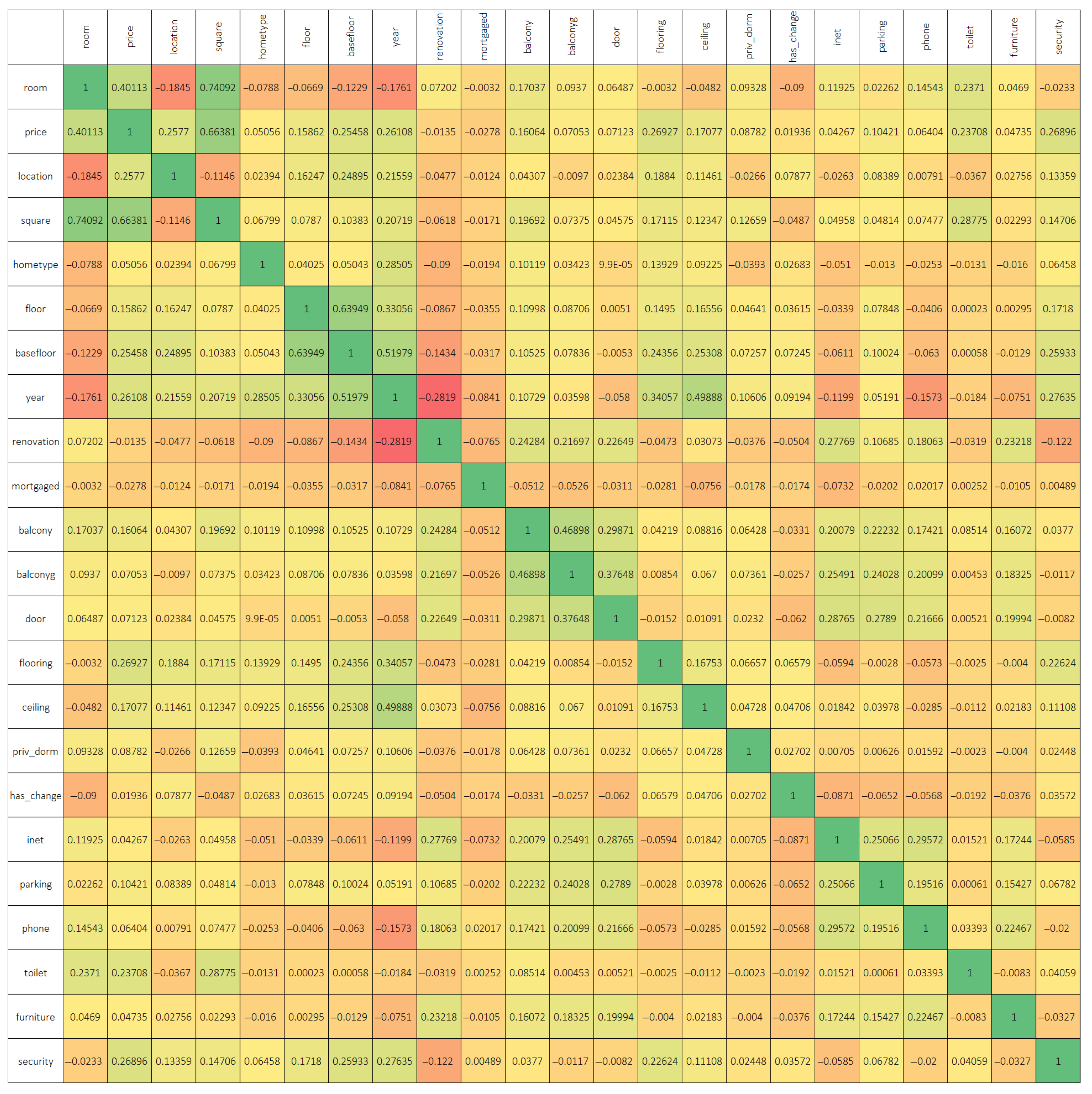
Table 1 presents a comprehensive statistical summary of various housing attributes, including the number of rooms, price, price per square meter, total area, home type, floor, year of construction, ceiling height, and security features. Each attribute is analyzed through several statistical measures. Average (mean) values indicate typical property characteristics within the dataset, with an average of 2.24 rooms and a mean price of approximately KZT 25.79 million. The average price per square meter stands at KZT 422,053.7, while the typical square meterage is 61.294 m2. Average values for home type, floor, year of construction, ceiling height, and security are also provided. Median values provide a midpoint of the data, reflecting a central trend where half of the houses have fewer than 2 rooms, a price less than KZT 23 million, and other median values for the remaining characteristics. Mode reflects the most frequently occurring value in each category, such as 2 rooms being the most common configuration and 60 m2 the most common area. Standard Deviation and Sample Variance provide insights into the dispersion of the data around the mean, with substantial variation observed in price and price per square meter. Skewness and Excess (Kurtosis) indicate the asymmetry and peakedness of the data distribution across different variables. Positive skewness in price and price per square meter suggests a tail towards higher values. High kurtosis in these variables indicates a concentration of values around the mean with heavy tails. Reliability Level (95%) provides the margin of error at a 95% confidence level, ensuring the precision of the estimates provided. This table forms a crucial part of the data analysis, providing a foundation for understanding the distribution and central tendencies of housing characteristics in the dataset. Figure 1 illustrates the correlation among various criteria affecting real estate prices.
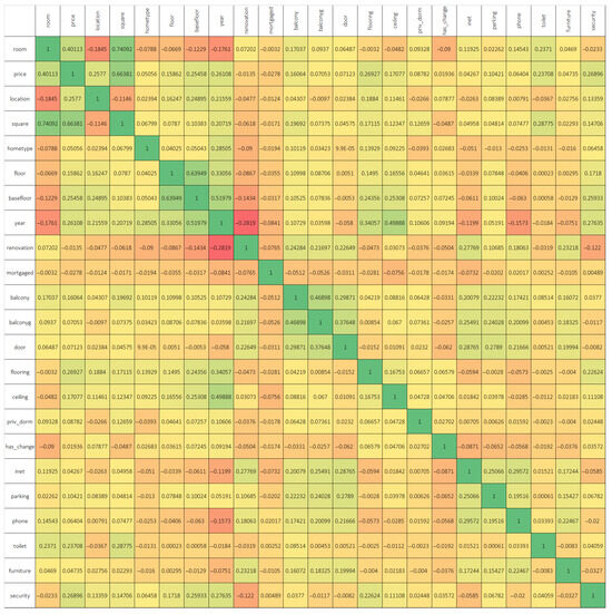
Figure 1.
Correlation of numerical indicators of real estate criteria. The heatmap shows correlations between variables, with green for strong positive correlations, red for strong negative correlations, and yellow/orange for weak or no correlation. The diagonal represents a perfect correlation of 1.
A strong correlation exists between the price of an apartment and its room size. Regional variations also significantly influence prices, with marked differences across different areas of the country. Additionally, the total area of an apartment (square footage) positively impacts its price. The data further reveal that newer buildings tend to house more expensive apartments. There is also a positive correlation between the number of bathrooms in an apartment, the level of security provided, and the corresponding price of the property. For investment strategies, the analysis suggests that purchasing apartments in specific regions with larger square footage at lower prices could be advantageous. For example, apartments requiring renovations generally obtain lower prices. Investors might consider acquiring properties with inexpensive flooring materials such as cork, wood, or linoleum, and upgrading to higher-quality materials like parquet or laminate to enhance value. Additionally, increasing the number of bathrooms and enhancing security measures could potentially increase the resale value of these properties. Among other notable correlations, the study observes that older buildings frequently contain apartments with smaller rooms, whereas newer constructions typically offer larger room sizes. There is also a trend towards constructing high-rise buildings, with these structures often featuring higher ceilings and enhanced security measures. Conversely, older buildings are more likely to contain apartments in poorer conditions.
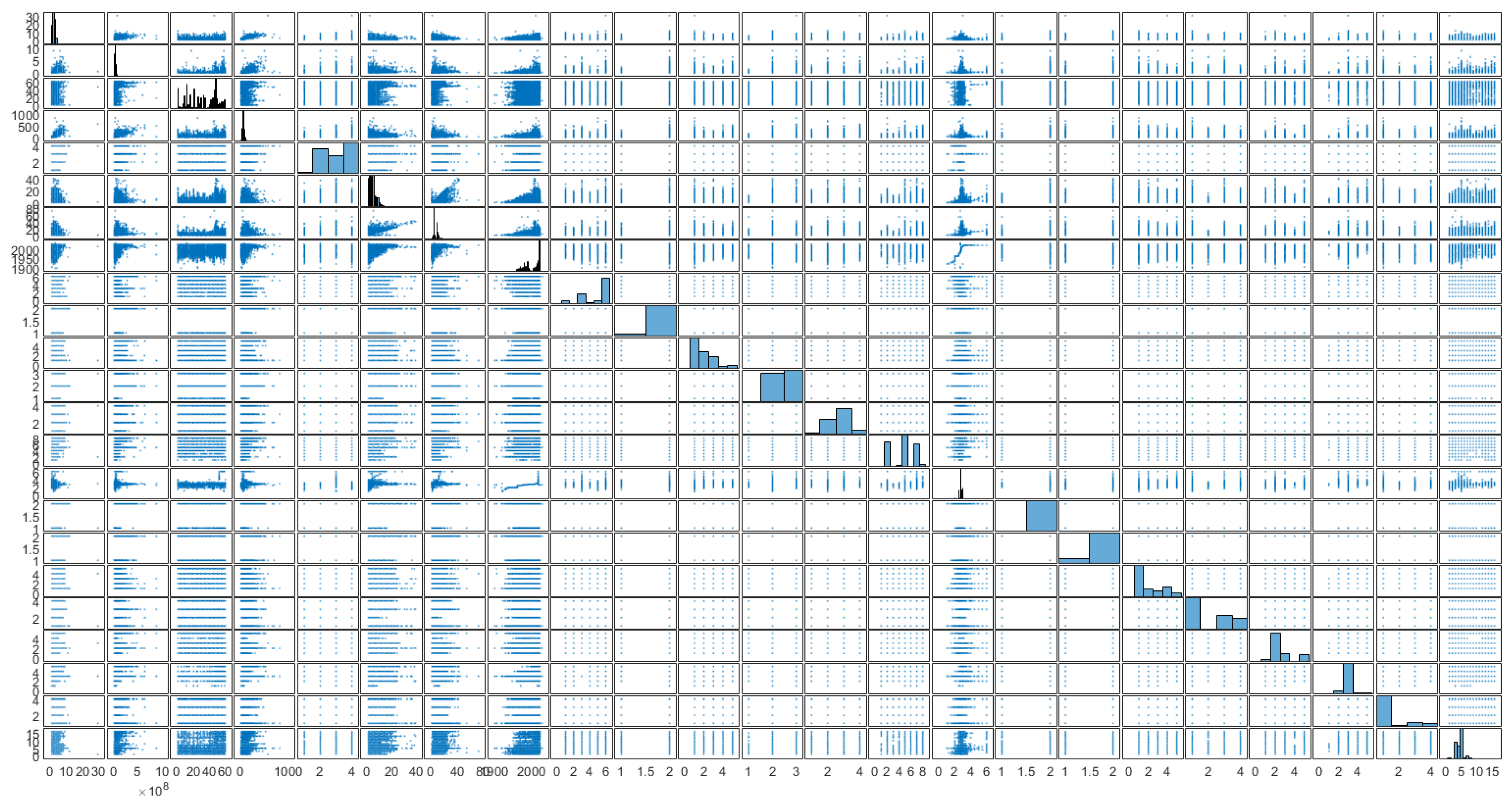
Figure 2, generated using the plotmatrix function, displays a matrix of scatter plots, with each plot comparing pairs of real estate criteria. The analysis of these plots reveals distinct regional variations in apartment prices, affirming a strong geographic influence on property values. Notably, apartments constructed with brick command the highest prices, followed by those in monolithic, panel, and other types of buildings, in descending order of price. The data also indicate an inverse relationship between building height and apartment prices; lower-rise buildings tend to house more expensive apartments compared to high-rise buildings, where apartments are generally cheaper. Additionally, newer constructions are associated with higher prices, reflecting a market preference for modern amenities and designs. The analysis further suggests that the quality of flooring materials significantly impacts pricing, with higher-quality materials correlating with higher prices. Contrarily, ceiling height appears to have no significant effect on apartment prices. However, an increase in the number of bathrooms and enhanced security features are both associated with higher property prices, indicating that these factors are valued in the housing market.
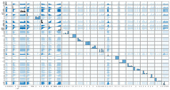
Figure 2.
Plotmatrix charts.
Figure 2 presents a comprehensive matrix of scatter plots and histograms systematically displaying the relationships and distributions among various real estate characteristics. Each subplot on the diagonal represents a histogram showing the distribution of a single variable, such as price, square footage, or the year of construction. Scatter plots off the diagonal illustrate the pairwise relationships between these variables. Variables like price and square footage display right-skewed distributions, suggesting a concentration of data at lower values with a tail extending towards higher values. The year of construction histogram indicates a multi-modal distribution, reflecting distinct periods of intensified building activity. The price-versus-square-footage scatter plot, located in the intersection corresponding to these two variables, shows a positive correlation, where larger properties tend to command higher prices. The correlation between the year of construction and price appears to be weaker, with newer properties occasionally fetching higher prices but with significant variability. Plots involving geographic location (not explicitly labeled here but typically represented) might show clusters, indicating price homogeneity within specific regions or variances in pricing trends across different areas. This plotmatrix is an effective tool for visually detecting trends, correlations, and distributions across multiple dimensions of data simultaneously. The presence of trends or outliers can quickly be assessed, providing a foundation for deeper statistical analysis or the development of predictive models. This matrix format allows researchers and analysts to grasp complex interrelationships and distributions without flipping through multiple charts, streamlining preliminary data exploration and hypothesis generation regarding real estate market behaviors.
2.2. Regression Techniques
In the analysis of our experimental data, regression techniques were implemented using MATLAB, a high-level programming and numeric computing environment. Linear regression was utilized to assess the strength and nature of the relationship between independent variables and a continuous dependent variable. The fitlm function in MATLAB facilitated the estimation of the coefficients by minimizing the sum of the squares of the residuals, providing a best-fit line to the observed data. The adequacy of the model fit was evaluated using the coefficient of determination, R2, and adjusted R2 values, along with F-statistics derived from an analysis of variance for the regression model. Multiple regression analysis was conducted when more than one independent variable was considered. The fitlm function was again employed, allowing for the assessment of each predictor’s unique contribution to the dependent variable, while controlling for the effects of other predictors. The significance of each predictor was examined through t-tests, and multicollinearity was assessed using variance inflation factors. For binary outcome variables, logistic regression was applied using the fitglm function, specifying a binomial distribution. This method provided probabilities of the outcome as a logistic function of the independent variables. The results included odds ratios with corresponding confidence intervals, and the model’s predictive accuracy was quantified by the area under the receiver operating characteristic curve. Non-linear relationships were modeled using the fitnlm function, which allowed for fitting arbitrary non-linear functions to the data. This method was particularly useful in cases where theoretical considerations suggested non-linear dynamics between variables. The iterative process adjusted parameters to minimize the residual sum of squares, and model fit was evaluated based on the residual analysis and goodness-of-fit measures such as Akaike’s Information Criterion. Polynomial regression was carried out to capture non-linear trends by fitting polynomial equations to the data. This was accomplished using the polyfit and polyval functions, which provided a polynomial model of a specified degree based on the least squares estimation.
2.3. Decision Tree Models and Neural Network Models
In our analysis, a diverse array of machine learning models was utilized to address the complexity of the data and the specific research questions posed. Utilizing MATLAB’s Statistics and Machine Learning Toolbox and Deep Learning Toolbox, we implemented various decision tree models and neural network architectures. The Fine Tree model, constructed using the fitctree function with ’MinLeafSize’ set to 1 allowed for very detailed data segmentation, leading to potentially complex models with high variance but low bias. This granularity was particularly useful for capturing subtle patterns in the data, although it increased the risk of overfitting. The Medium Tree model, also built with fitctree, used a default ’MinLeafSize’ of 10. This setting provided a balance between model complexity and generalizability, making it suitable for our datasets where a moderate level of data detail was sufficient for effective analysis. The Coarse Tree model was configured with a ’MinLeafSize’ of 20 using fitctree. This model was designed to be less sensitive to the noise in the data, producing simpler models that are more robust but potentially underfitted on very complex datasets. Boosted Trees were implemented using the fitcensemble function with ’Method’ set to ’AdaBoostM1’. This technique combines multiple weak learners (typically decision trees) into a strong learner by focusing on instances that were misclassified in previous trees, thereby improving the model’s accuracy on difficult cases. Bagged Trees, or Bootstrap Aggregated Trees, were constructed using TreeBagger. This method reduces variance and helps avoid overfitting by creating each tree from a bootstrap sample of the data and averaging the results. The Narrow Neural Network was designed with a single hidden layer containing 10 neurons, utilizing the patternnet function. This configuration, optimized for less complex patterns, reduces the computational burden while providing sufficient capacity to model basic relationships in the data. The Medium Neural Network featured a single hidden layer of 25 neurons, constructed using patternnet. This model offered a good trade-off between complexity and performance, suitable for datasets with moderate intricacies. The Wide Neural Network, with a first hidden layer of 100 neurons, was also designed using patternnet. This architecture was intended to capture more complex patterns and interactions in the data at the cost of increased computational demand and a higher risk of overfitting. The Bilayered Neural Network consisted of two hidden layers, each containing 10 neurons, configured using patternnet. This setup allowed the model to learn more complex features at the first layer and abstract these features further in the second layer, enhancing the model’s ability to generalize from more complex data structures.
2.4. Decision Tree Models and Neural Network Models
In this study, we employed ANFIS, a hybrid model that combines neural networks with fuzzy logic principles, to capture the underlying functional relationships within the dataset. ANFIS is particularly adept at modeling complex non-linear functions that are difficult to model with traditional techniques due to its ability to approximate any continuous function arbitrarily well. The ANFIS model utilizes a Takagi–Sugeno-type fuzzy inference system, which is implemented in a framework similar to a feedforward neural network. This system includes five layers: a fuzzification layer, a rules layer, a normalization layer, a defuzzification layer, and a total output layer. Each of these plays a critical role in processing inputs through the network to produce a crisp output. In the first layer, input variables are matched with membership functions (MFs) that are typically Gaussian, bell-shaped, or triangular. These functions assign a membership value between 0 and 1 to each input, determining the degree to which inputs belong to in each of the appropriate fuzzy sets. The second layer involves the application of fuzzy logic rules, which are typically of the form “If-Then” statements. The outputs of this layer are the product of the input membership values applied to each rule, representing the fired strength of the rules. The third layer normalizes the rule strengths from the previous layer, dividing each rule’s output by the sum of all rule outputs. This ensures that the sum of all outputs from this layer equals 1, setting the stage for a combination in subsequent layers. In the fourth layer, each rule’s output is multiplied by the function it maps to (usually a linear function of the inputs). This layer produces a weighted output for each rule based on the normalized firing strengths. The final layer sums all incoming signals from the defuzzification layer to produce a single output from the system. The ANFIS model was trained using a hybrid learning rule that combines the least squares method and the backpropagation gradient descent method. This approach allows for the efficient and precise tuning of membership function parameters to minimize a specified error function, typically the mean-squared error between the predicted and actual values. To validate the ANFIS model, we employed k-fold cross-validation. This method involves dividing the dataset into k subsets and iteratively training the model on k − 1 subsets while using the remaining subset for validation. This technique not only provides insights into the model’s generalizability but also helps in identifying overfitting issues. The performance of the ANFIS model is highly dependent on the structure and parameters of the membership functions. We optimized these parameters, including the number of rules and the type of membership functions, using grid search and genetic algorithms to find the best combination that minimizes the prediction error.
3. Results
3.1. Analysis of the Real Estate Market by Regression Learner
To build regression learner models, we used Matlab, which has a very user-friendly interface [37]. Table 2 shows the results of regression learner models. For a better regression calculation, we divided the price value by one million, for example, 18,000,000 = 18 million. As an output parameter, we also set the values of the price column, and in the second case as an output parameter, we set the values of the price per square meter column. In the calculations, we used 12 forecast models. The results of the models in the table show the performance of each model on a regression task. The models are compared based on four performance metrics: RMSE, R-squared, MSE, and MAE. The data in the table suggest that the Bagged Tree model yielded the best results in terms of both RMSE and MAE for price. It also showed good performance against the price per square meter criterion, with its smallest RMSE value and a relatively high R value. The Bagged Tree model and the Fine and Medium Tree models exhibited relatively low RMSE and MAE scores for the price criterion. Additionally, they also displayed satisfactory performance when tested against the price per square meter criterion. The Boosted Tree model offered a reasonably low RMSE for the square meter price; however, its performance on the actual price was not as impressive compared to other models. The Medium Neural Network (MNN) and Wide Neural Network (WNN) models showed impressive performance in terms of accuracy when predicting the price. They had relatively low RMSE and MAE for the price criteria, and satisfactory results for the price per square meter criterion. Narrow Neural Network (NNN) and Bilayered Neural Network (BFANN) models were both fairly efficient with similar performance results. However, when it comes to the price criterion, they had a slightly increased root-mean-squared error (RMSE) and mean absolute error (MAE).
Table 2.
Regression models in determining the value of real estate.
Overall, the Bagged Tree model stands out as the best performer for both price and price per square meter criteria. However, it is always a good idea to try out multiple models and compare their performance to ensure the best possible results.
Table 2 presents a comprehensive comparison of various regression models used to predict real estate values, analyzed based on two output parameters: the price and price per square meter criteria. The LR model shows moderate accuracy with an RMSE of 11.549 for the price criterion and 142.83 for price per square meter, indicating a lower fit for the latter. The ILR model improves upon the linear regression model, achieving a higher correlation coefficient of 0.68 and 0.4 for the two output parameters, respectively. The RLR model shows varied performance with generally lower R values compared to ILR. Decision tree models show improvements over linear models with Fine Tree providing the lowest RMSE values, indicating a better fit. The performance consistency across the tree models highlights their effectiveness in handling non-linear data relationships. Ensemble models leverage multiple learning algorithms to obtain better predictive performance, with Bagged Trees showing the best results in terms of both RMSE and R, particularly for the price criterion. The performance tends to improve with wider or more complex neural networks, as indicated by the gradual increase in R values and decrease in RMSE. Bagged Tree model shows the best overall performance for predicting price, with the lowest RMSE (7.9794) and highest R (0.81). For price per square meter, Bagged Trees again show the best performance with an RMSE of 98.46 and R of 0.69. Decision tree models generally perform well, suggesting that the data may have a non-linear structure that these models can effectively capture. Neural networks show variable performance, but the more complex models (e.g., Wide and Bilayered) generally provide better accuracy.
3.2. Analysis of the Real Estate Market by Neural Networks
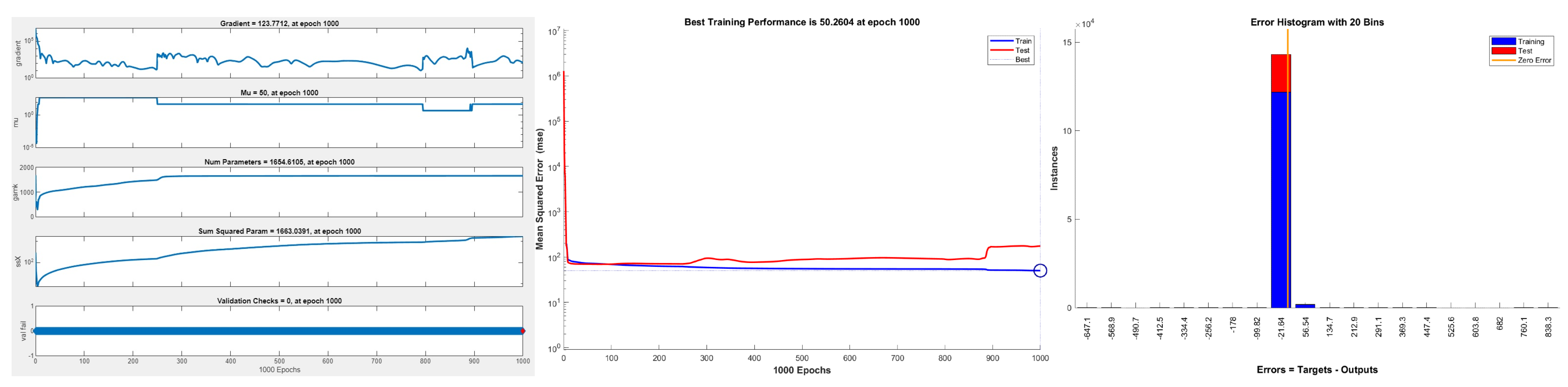
In order to obtain an improved model, we decided to analyze the data using a deep learning model which uses Bayesian regularization to avoid overfitting. After running the model with 70 layers and the Bayesian regularization algorithm (BR-BPNN), it was observed that the training MSE was 50.2604 and the training R value was 0.9197. Examining the metrics, it is clear that the model was successful in recognizing patterns and relationships in the training dataset. This implies that it has a good fit for this dataset and is capable of making accurate predictions. The results are shown in Figure 3 and Figure 4.
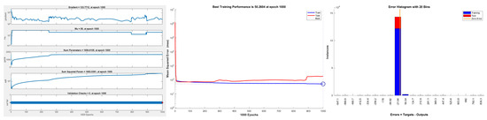
Figure 3.
Neural network performance graphs.
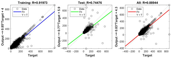
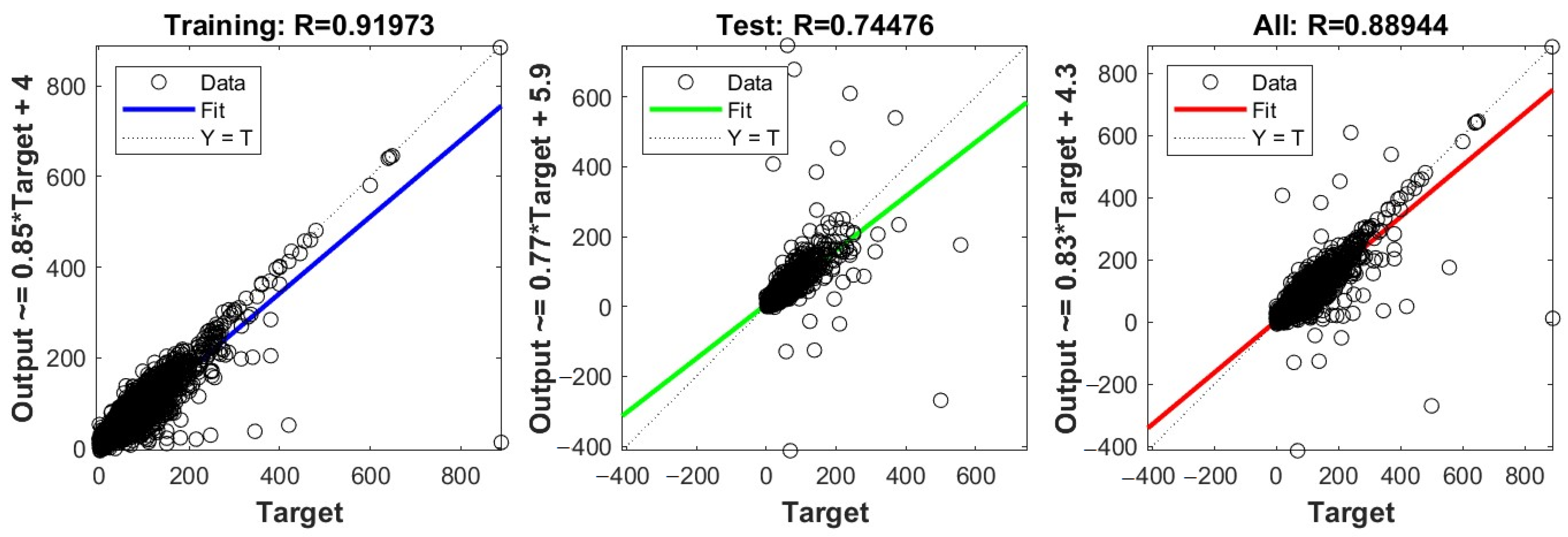
Figure 4.
Regression plot of a neural network model with output parameters’ price.
The test results were not as promising as expected. Specifically, the mean-squared error (MSE) of 21,778 showed that the model’s predictions were diverging from the true data values in the test dataset by a sizeable amount. The R value of 175.3564 is especially high, which implies that something is not right with the appraisal since R values are usually between −1 and 1.
Due to the small size of the test dataset, at 0.7448 observations, a large variation in the results of the test is understandable. To obtain more reliable results from unseen data, it may be necessary to collect additional data.
After a comprehensive evaluation of the training results, it has been concluded that the neural network has the capacity to operate well. However, further development may be necessary to enhance its capacity to generalize fresh data. To obtain the most out of our AI model, we may need to tweak its hyperparameters or use a different algorithm altogether. We can also evaluate the performance of our model by testing it with larger datasets. Doing so can give us a better indication as to how well it performs in real-world scenarios. Next, we want to use fuzzy logic to build a fuzzy expert real estate valuation system [38,39].
The series of figures provide a comprehensive visualization of the training and validation of a machine learning model over 1000 epochs. The figures include various metrics and parameter changes, facilitating an understanding of model behavior and performance over time. The first graph shows the gradient magnitude across epochs, indicating how the model’s gradients evolve, which affects learning rates and convergence. The graph holds the value of Mu (momentum) constant, and is used to accelerate convergence in a gradient descent. The number of parameters and their sum are squared values, respectively, providing insight into the model’s complexity and weight adjustments throughout the training process. The second graph displays the MSE for both training and testing datasets over 1000 epochs. A marked decrease in MSE is observed initially, stabilizing as the epochs increase, with a minimal gap between training and testing errors, suggesting a good generalization of the model. The final graph presents an error histogram with 20 bins, showing the distribution of errors between predicted outputs and actual targets. The majority of errors cluster near zero, indicating that most predictions are close to the target values. The presence of few large errors suggests occasional deviations from the target values. The stability of the gradient over time suggests effective learning rates, while the constant Mu indicates a set momentum that might have been optimized for this particular training. The steady increase in the number of parameters and their squared sums could imply a complex model that potentially captures a detailed representation of the underlying data patterns. The error histogram and training performance graphs together validate the model’s ability to learn and generalize well, with errors predominantly concentrated near zero and a low and stable MSE across epochs.
Figure 4 presents regression plots for training, testing, and the combined dataset, each illustrating the relationship between target values (x-axis) and model outputs (y-axis). The training data regression plot (first plot) shows a correlation coefficient of 0.91973, indicating a strong positive correlation between the target and the output values during training. The blue line represents the regression line, suggesting a close fit to the ideal line (Y = T, dotted line), where output equals target, depicting the model’s high accuracy in the training phase. Data points mostly cluster along the regression line, showing good model prediction accuracy with training data.
The testing data regression plot (second plot) shows a correlation coefficient of 0.74476, and demonstrates a moderate positive correlation, which is notably lower than the training phase, indicating possible overfitting or the model’s decreased performance on unseen data. The green fit line deviates more from the Y = T line compared to the training phase, indicating less accuracy with testing data. The data points are more spread out from the line of best fit, suggesting higher variability and lower prediction accuracy.
The combined data regression plot (third plot) shows a correlation coefficient of 0.88944, reflecting a high positive correlation, showing that overall, the model performs well across the entire dataset. The red line is closer to the ideal Y = T line, indicating better performance across the combined dataset compared to just the testing set. The data points display a dense clustering along the regression line but with noticeable spread, highlighting areas where model performance may vary.
The plots effectively illustrate how well the model has learned to predict the outcomes relative to the actual target values across different data subsets. The high correlation in the training data suggests a good model fit, while the drop in correlation in the testing data highlights potential overfitting or the model’s limitations when generalized to new data. The combined data analysis helps in understanding the overall effectiveness of the model across all data points, providing a holistic view of performance.
3.3. Analysis of the Real Estate Market by Adaptive Neuro-Fuzzy Inference System
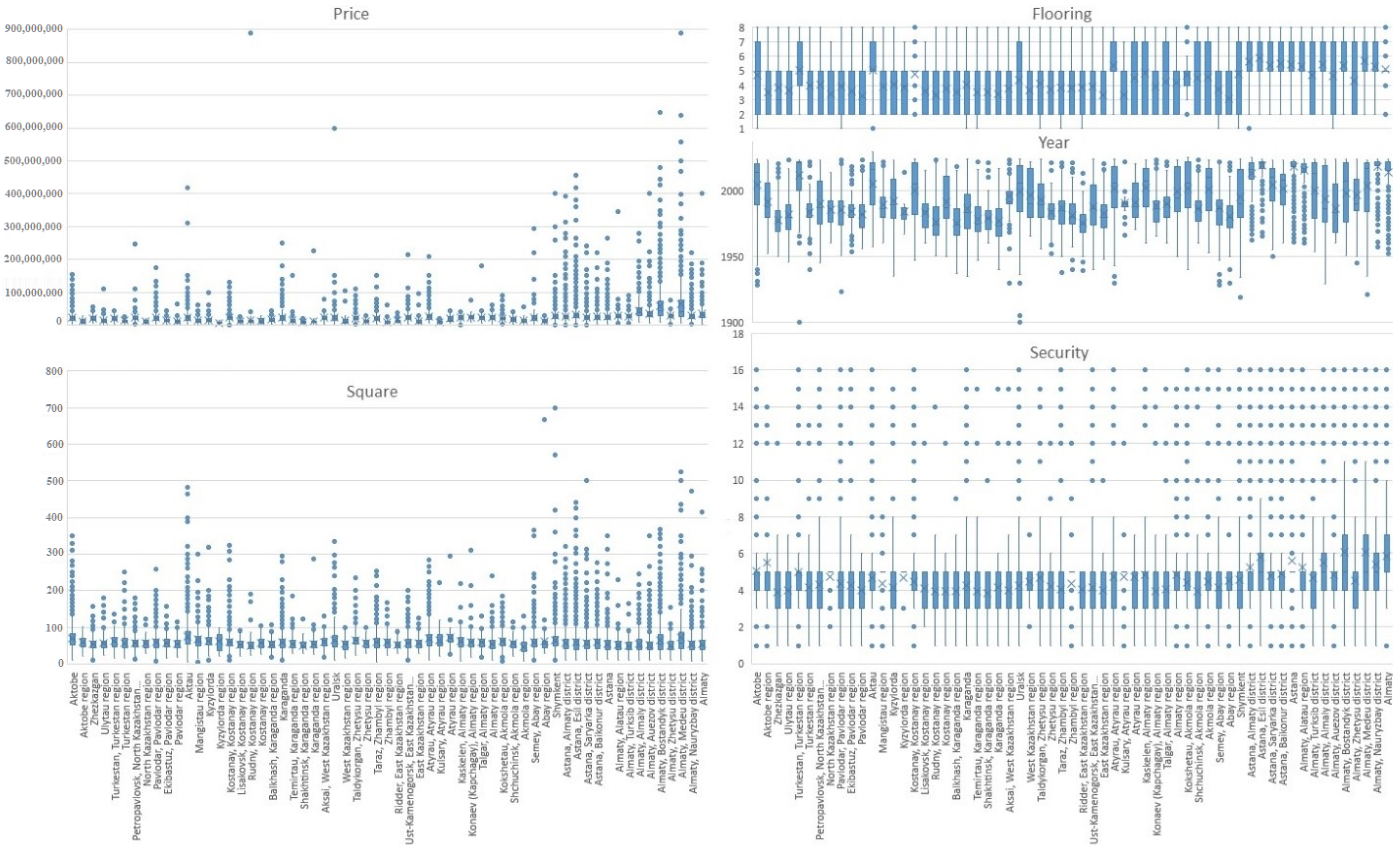
To build a fuzzy neural network model, we can only use three to four input parameters. Analyzing Figure 1 and Figure 2, we conclude that the price is mainly influenced by criteria: number of rooms = 0.40113, square = 0.66381, year of construction = 0.26108, floor material = 0.26927, and security level = 0.26896. Figure 5 shows how these criteria are distributed in different regions of the country. The most expensive apartments are located in the Medeu district of Almaty, followed by the Bostandyk district of Almaty, Esil district of Astana, Almaty district of Astana, Shymkent, and the Auezov district of Almaty. The largest apartments are located in Shymkent, the Medeu district of Almaty, Aktau, and the Esil district of Astana. The best security is found in Medeu and Bostandyk districts of Almaty. The number of rooms and the square have a close semantic value. Therefore, it was decided to use the square parameter, since it has a stronger correlation with the price criterion. As input parameters for ANFIS, we will use the following: square, year, flooring, and security. As an output variable for ANFIS, we will use the price criterion.
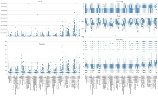
Figure 5.
Box plots of price, square, flooring, year, and security in relation to the location.
With an input/output dataset, the ANFIS toolbox function can develop a fuzzy inference system (FIS) with membership function [40] parameters adjusted using backpropagation or a least squares type of method. This offers efficient tuning to achieve the desired output. By integrating fuzzy systems, data can be utilized to learn patterns and be modeled accordingly. This ultimately increases efficiency and accuracy. The basics of neuro-adaptive learning are straightforward and easy to understand. These techniques enable faster, better and more accurate learning outcomes. By using these techniques, it is possible to apply fuzzy modeling to learn about datasets and compute the membership function parameters which enable the fuzzy inference system to accurately estimate input/outputs. This allows for the successful execution of a reliable fuzzy modeling procedure. This learning strategy is quite similar to the one employed by neural networks. J.-S. Roger Jang’s algorithm, developed in 1992, formed a fuzzy decision tree to classify data into one of 2n (or pn) linear regression models, leading to a minimal sum of squared errors (SSEs). , where ej is the error between the desired and the actual output, p is the number of fuzzy partitions of each variable, and n is the number of input variables. A fuzzy neural network model has 193 nodes, 81 linear parameters, 36 non-linear parameters, and 81 fuzzy rules. The training results are shown in Figure 6. The RMSE of the ANFIS model is 5.80874. A comparison of ANFIS with other machine learning models is shown in Figure 7.
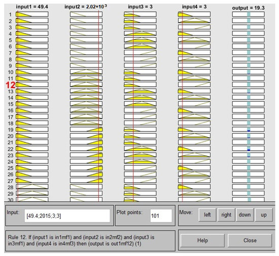
Figure 6.
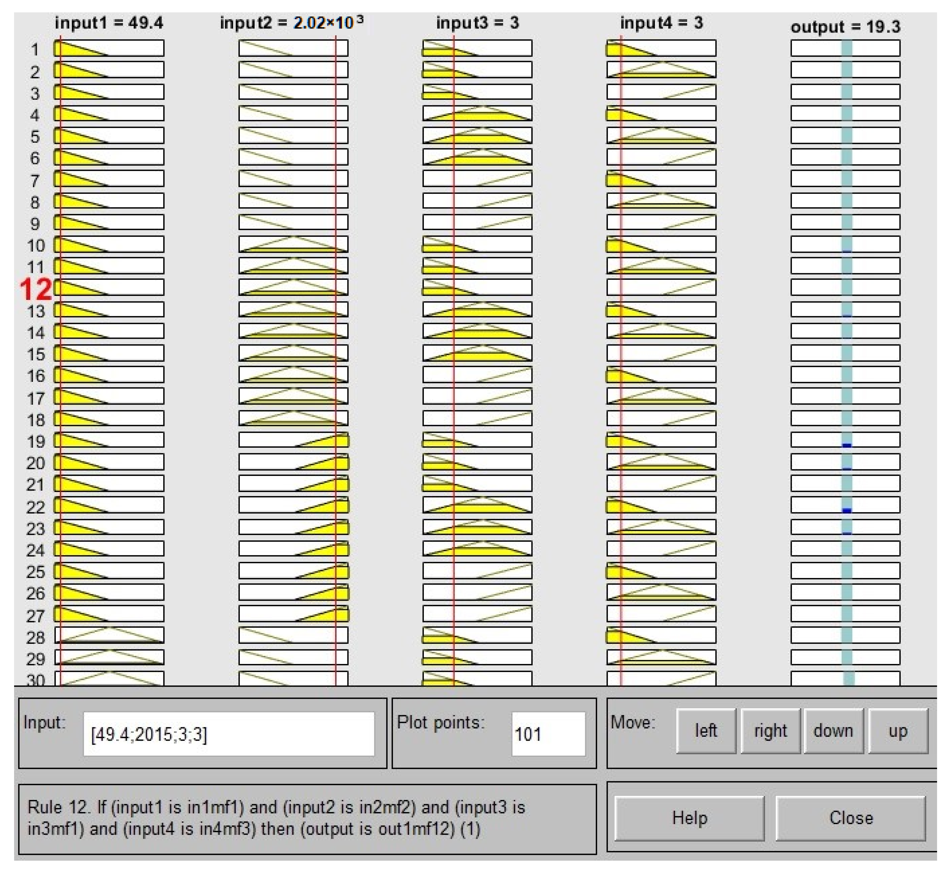
Fuzzy expert system. The yellow and red areas represent membership function activations, and the blue indicates the corresponding output region.

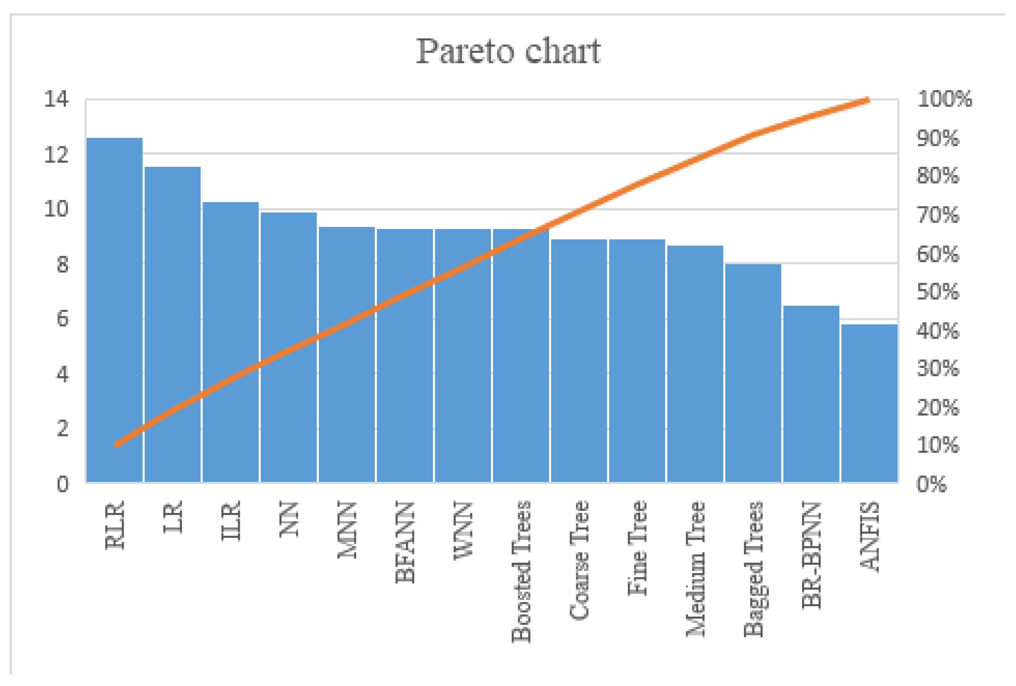
Figure 7.
Comparison of ML models. The bar chart shows the performance of various machine learning models, with the minimum value representing the best efficiency. The orange line represents the cumulative percentage contribution of these models to overall performance.
Figure 6 illustrates a graphical representation of a fuzzy logic controller or a rule-based system, and is used in machine learning or control systems to map given inputs to outputs based on predefined rules. Each column represents different variables (inputs and outputs) with their corresponding membership functions distributed across rows, depicted as lines. The highlighted paths indicate active rules and their influence for a specific set of input values. There are four input variables (input1 to input4) and one output variable (output), each divided into multiple fuzzy membership functions (MFs) represented as rows. The specific values for this instance are provided at the top as input1 = 49.4, input2 = 2020, input3 = 3, input4 = 3, and output = 19.3. Each input and output variable is associated with several MFs, which categorize the inputs and outputs into linguistic terms like low, medium, high, etc., visualized through different levels or rows in each column. Highlighted in yellow, these paths show the active routes through the MFs based on the current inputs. The paths link specific MFs across the input variables to a corresponding MF of the output variable. The highlighted rule (Rule 12) at the bottom specifies a conditional logic that connects these input values to the resultant output. It states, “if [conditions on inputs], then [specific output].” This rule and its activation are further evidenced by the yellow lines which connect the dots (MF levels) across the inputs to the output, suggesting which MFs are activated according to the rule’s logic. This visualization helps in understanding the complex relationships and decision-making processes within a fuzzy logic system by showing which rules are triggered under certain conditions and how input values translate into a specific output through logical inference.
This particular Pareto chart evaluates various regression models according to a metric, likely reflecting performance or error rates. The chart combines a bar graph and a cumulative percentage line to display the importance and impact of each model. Each bar represents a different regression model, with the height indicating the metric’s value, which could be the error rate, accuracy, or another performance measure. The models are ordered from left to right by decreasing value of the metric. The cumulative percentage line traces the cumulative percentage of the total sum of the metric across the models. It starts at the top-left, indicating that the first model contributes a significant percentage to the total metric value, and it increases as it moves to the right.
The analysis of the dataset employed for investigating apartment sales in Kazakhstan is ostensibly thorough; however, certain potential limitations were not explicitly articulated within the document. The data were extracted at a singular temporal point, which may not encapsulate seasonal fluctuations or longitudinal trends within the real estate market. Although the dataset encompasses a broad spectrum of apartment characteristics, it potentially excludes critical factors such as the economic vitality of the neighborhood, prospective development initiatives, and additional socio-economic indicators that might significantly influence apartment prices. A comprehensive understanding of these limitations is imperative for an accurate interpretation of the study’s findings and could provide a foundation for future research aimed at addressing these deficiencies.
Future research endeavors predicated on the analysis of the Kazakhstan real estate market ought to contemplate several advanced and nuanced avenues to enrich our comprehension and augment the precision of market forecasts. Prospective studies should endeavor to collect data across multiple temporal junctures to scrutinize seasonal and cyclical effects on the real estate market, thereby facilitating the development of more dynamic and robust forecasting models. Moreover, broadening the dataset to encompass additional regions within Kazakhstan or facilitating comparisons with international markets could yield deeper insights into regional disparities and the influence of global economic trends on local real estate dynamics. Furthermore, the integration of socio-economic indicators, such as income levels, demographic transitions, and economic policies, could significantly enhance the model’s predictive capabilities by correlating real estate trends with broader macroeconomic conditions. Pursuing these research directions could profoundly augment our understanding of real estate dynamics, consequently leading to more informed decision-making and policy development.
4. Discussion
This study has systematically evaluated the efficacy of various predictive models in the context of real estate valuation in Kazakhstan, with a particular focus on ANFIS. Our findings reveal that while traditional models such as linear regression and decision trees provide baseline accuracy, ANFIS offers superior precision due to its capability to model non-linear relationships and handle data imprecision effectively. The performance of the ANFIS model stands out when compared to traditional econometric and machine learning models. Unlike linear models that assume a direct correlation between variables, ANFIS integrates the advantages of fuzzy logic and neural networks, accommodating the inherent uncertainties of the real estate market. This integration enables ANFIS to capture complex patterns that are typically missed by other models, as demonstrated by its lower RMSE and higher R-values. The application of ANFIS can significantly enhance the accuracy of property valuations, which is critical for investors, policymakers, and financial analysts involved in real estate development and market analysis. By providing a more reliable tool for valuation, ANFIS helps in better assessing property values, thus supporting more informed decision-making processes. While our results are promising, they are not without limitations. The models were tested within the specific context of Kazakhstan’s real estate market, and their applicability in other markets might differ due to varying economic and regulatory conditions. Future research could expand the application of ANFIS to other regions and compare its effectiveness across different economic contexts. Additionally, incorporating more dynamic data, such as time series analysis of property prices, could further refine the predictive capabilities of these models. Integrating ANFIS into real estate valuation practices could pave the way for standardizing property appraisal methods, reducing the subjectivity involved in manual valuations. Policymakers might consider these findings when updating regulatory frameworks to adopt more scientific and data-driven approaches for property valuation.
5. Conclusions
The current study offers valuable insights for investors seeking to optimize returns on apartment investments. Targeting properties in regions where larger apartments are undervalued, particularly those requiring renovations, presents a viable investment strategy. Enhancements such as upgrading to higher-quality flooring materials, increasing the number of bathrooms, and improving security measures can significantly elevate property values. Additionally, the study identifies the age of the building and the construction material, specifically, the higher costs associated with brick constructions and the lower prices attributed to high-rise buildings as critical factors influencing resale values. Through the deployment of an advanced deep learning model encompassing 70 layers and Bayesian regularization, the study successfully discerned intricate patterns and relationships within the dataset. This model demonstrated robust performance, indicated by a training MSE of 50.2604 and an R of 0.9197. The application of ANFIS further refined our predictive accuracy, as evidenced by its superior metrics over 1000 training epochs: an RMSE of 5.80874, R of 0.9354, MSE of 39.1298, and MAE of 2.7582—surpassing other evaluated models. The comparative analysis across various machine learning models highlighted the efficacy of ANFIS and underscored its superior capability in minimizing prediction errors and enhancing correlation strength between predicted and actual values. ANFIS uniquely integrates the advantages of both fuzzy logic and neural networks, enabling the handling of uncertain data and learning complex, non-linear relationships with remarkable precision. This hybrid model, therefore, stands out as particularly suitable for predictive tasks where data intricacy and uncertainty are prevalent. While linear regression provides a simpler, more interpretable modeling approach, it often falls short in non-linear scenarios where the assumptions of linear relationships do not hold. Conversely, tree-based models like Boosted Trees, Medium Tree, and Fine Tree adeptly handle these non-linear relationships. Neural networks, despite their higher computational demands, offer significant advantages in capturing complex interactions between variables. In contrast, fuzzy logic-based models excel in managing uncertainty and imprecision, making them ideal for specific applications. The ANFIS model not only outperformed other models in predictive accuracy but also demonstrated its utility in real-world applications, such as estimating the market value of secondary housing. This study’s findings advocate for the use of ANFIS in complex predictive tasks, offering a robust tool for investors and policymakers in the real estate valuation domain. The selection of an appropriate model, however, should ultimately align with the specific data characteristics and application requirements, balancing complexity, interpretability, and computational efficiency.
Author Contributions
Conceptualization, A.B., N.O. and A.S.; methodology, N.O., A.S. and B.M.; software, N.O.; validation, A.S. and B.M.; formal analysis, A.B.; investigation, A.B., N.O. and B.M.; resources, A.B. and N.O.; data curation, N.O. and A.S.; writing—original draft preparation, A.B. and A.S.; writing—review and editing, A.B. and N.O.; visualisation, N.O. and A.S.; supervision, A.S. and B.M.; project administration, B.M.; funding acquisition, A.B. All authors have read and agreed to the published version of the manuscript.
Funding
This research was funded by the Science Committee of the Ministry of Science and Higher Education of the Republic of Kazakhstan (grant no. of the research fund: AP23489994).
Institutional Review Board Statement
Not applicable.
Informed Consent Statement
Not applicable.
Data Availability Statement
The original contributions presented in this study are included in the article; further inquiries can be directed to the corresponding authors.
Conflicts of Interest
The authors declare no conflicts of interest. The funders had no role in the design of the study; in the collection, analyses, or interpretation of data; in the writing of the manuscript; or in the decision to publish the results.
References
- Draper, N.R.; Smith, H. Applied Regression Analysis; Wiley: New York, NY, USA, 1967. [Google Scholar]
- Eckert, J. Organization of Real Estate Valuation and Taxation: In 2 Volumes; Star Inter: Moscow, Russia, 1997. (In Russian) [Google Scholar]
- Zaks, L. Statistical Evaluation; Statistika: Moscow, Russia, 1976. (In Russian) [Google Scholar]
- Sternik, G.M.; Sternik, S.G. Evaluation of the mid-market investment returns in real estate development when forecasting the housing market. Stud. Russ. Econ. Dev. 2017, 28, 204–212. [Google Scholar]
- French, N.; Gabrielli, L. Pricing to market: Property valuation revisited: The hierarchy of valuation approaches, methods and models. J. Prop. Investig. Financ. 2018, 36, 391–396. [Google Scholar]
- Court, L.M. Entrepreneurial and consumer demand theories for commodity spectra: Part I. Econom. J. Econom. Soc. 1941, 9, 135–162. [Google Scholar] [CrossRef]
- Tinbergen, J. Some remarks on the distribution of labour incomes. In International Economic Papers; Translations prepared for the International Economic Association; Peacock, A.T., Houthakker, H.S., Lutz, F.A., Henderson, E., Eds.; Macmillan: London, UK, 1951; p. 1. [Google Scholar]
- Rosen, S. Hedonic prices and implicit markets: Product differentiation in pure competition. J. Political Econ. 1974, 82, 34–55. [Google Scholar] [CrossRef]
- Sheppard, S. Hedonic analysis of housing markets. In Handbook of Regional and Urban Economics; Mills, E.S., Cheshire, P., Eds.; Elsevier: Amsterdam, The Netherlands, 1999; Volume 3, pp. 1595–1635. [Google Scholar]
- Pinter, G. House prices and job losses. Econ. J. 2019, 129, 991–1013. [Google Scholar] [CrossRef]
- Badarinza, C.; Ramadorai, T. Home away from home? Foreign demand and London house prices. J. Financ. Econ. 2018, 130, 532–555. [Google Scholar]
- Kelly, R.; McCann, F.; O’Toole, C. Credit conditions, macroprudential policy and house prices. J. Hous. Econ. 2018, 41, 153–167. [Google Scholar]
- Agnello, L.; Castro, V.; Hammoudeh, S.; Sousa, R.M. Spillovers from the oil sector to the housing market cycle. Energy Econ. 2017, 61, 209–220. [Google Scholar] [CrossRef]
- Monnet, E.; Wolf, C. Demographic cycles, migration and housing investment. J. Hous. Econ. 2017, 38, 38–49. [Google Scholar]
- Jim, C.Y.; Chen, W.Y. Impacts of urban environmental elements on residential housing prices in Guangzhou (China). Landsc. Urban Plan. 2006, 78, 422–434. [Google Scholar]
- Sing, T.F. Dynamics of the condominium market in Singapore. Int. Real Estate Rev. 2001, 4, 135–158. [Google Scholar] [CrossRef] [PubMed]
- Zhang, L.; Yi, Y. What contributes to the rising house prices in Beijing? A decomposition approach. J. Hous. Econ. 2018, 41, 72–84. [Google Scholar] [CrossRef]
- Portnov, B.A.; Odish, Y.; Fleishman, L. Factors affecting housing modifications and housing pricing: A case study of four residential neighborhoods in Haifa, Israel. J. Real Estate Res. 2005, 27, 371–408. [Google Scholar] [CrossRef]
- d’Albis, H.; Boubtane, E.; Coulibaly, D. International migration and regional housing markets: Evidence from France. Int. Reg. Sci. Rev. 2019, 42, 147–180. [Google Scholar] [CrossRef]
- Fan, C.; Cui, Z.; Zhong, X. House prices prediction with machine learning algorithms. In Proceedings of the 2018 10th International Conference on Machine Learning and Computing, Macau, China, 26–28 February 2018; pp. 6–10. [Google Scholar]
- Phan, T.D. Housing price prediction using machine learning algorithms: The case of Melbourne city, Australia. In Proceedings of the 2018 International Conference on Machine Learning and Data Engineering (iCMLDE), Melbourne, Australia, 3–7 December 2018; pp. 35–42. [Google Scholar]
- Ma, C.; Liu, Z.; Cao, Z.; Song, W.; Zhang, J.; Zeng, W. Cost-sensitive deep forest for price prediction. Pattern Recognit. 2020, 107, 107499. [Google Scholar] [CrossRef]
- Wang, P.Y.; Chen, C.T.; Su, J.W.; Wang, T.Y.; Huang, S.H. Deep learning model for house price prediction using heterogeneous data analysis along with joint self-attention mechanism. IEEE Access 2021, 9, 55244–55259. [Google Scholar] [CrossRef]
- Zulkifley, N.H.; Rahman, S.A.; Ubaidullah, N.H.; Ibrahim, I. House price prediction using a machine learning model: A survey of literature. Int. J. Mod. Educ. Comput. Sci. 2020, 12, 46–54. [Google Scholar] [CrossRef]
- Gao, G.; Bao, Z.; Cao, J.; Qin, A.K.; Sellis, T. Location-centered house price prediction: A multi-task learning approach. ACM Trans. Intell. Syst. Technol. (TIST) 2022, 13, 1–25. [Google Scholar] [CrossRef]
- Trang, L.H.; Huy, T.D.; Le, A.N. Clustering helps to improve price prediction in online booking systems. Int. J. Web Inf. Syst. 2021, 17, 45–53. [Google Scholar] [CrossRef]
- Rizun, N.; Baj-Rogowska, A. Can web search queries predict price changes on the real estate market? IEEE Access 2021, 9, 70095–70117. [Google Scholar] [CrossRef]
- Liu, G. Research on prediction and analysis of real estate market based on the multiple linear regression model. Sci. Program. 2022, 2022, 5750354. [Google Scholar] [CrossRef]
- Wiradinata, T.; Tanamal, R.; Saputri, T.R.; Soekamto, Y.S. An implementation of support vector machine classification for developer academy acceptance prediction model. In Proceedings of the 2021 2nd International Conference on Innovative and Creative Information Technology (ICITech), Jakarta, Indonesia, 23–25 September 2021; pp. 110–116. [Google Scholar]
- Shinde, N.; Gawande, K. Valuation of house prices using predictive techniques. J. Adv. Electron. Comput. Sci. 2018, 5, 34–40. [Google Scholar]
- Gerek, I.H. House selling price assessment using two different adaptive neuro-fuzzy techniques. Autom. Constr. 2014, 41, 33–39. [Google Scholar] [CrossRef]
- Jiang, L.; Liao, H. Mixed fuzzy least absolute regression analysis with quantitative and probabilistic linguistic information. Fuzzy Sets Syst. 2020, 387, 35–48. [Google Scholar] [CrossRef]
- Chachi, J.; Kazemifard, A.; Jalalvand, M. A multi-attribute assessment of fuzzy regression models. Iran. J. Fuzzy Syst. 2021, 18, 131–148. [Google Scholar]
- Mukhlishin, M.F.; Saputra, R.; Wibowo, A. Predicting house sale price using fuzzy logic, artificial neural network and K-nearest neighbor. In Proceedings of the 2017 1st International Conference on Informatics and Computational Sciences (ICICoS), Bali, Indonesia, 15–16 November 2017; pp. 171–176. [Google Scholar]
- Barlybayev, A.; Sankibayev, A.; Niyazova, R.; Akimbekova, G. Machine learning for real estate valuation: Astana, Kazakhstan case. Indones. J. Electr. Eng. Comput. Sci. 2024, 35, 1110–1121. [Google Scholar] [CrossRef]
- Omarbekova, A.; Sharipbay, A.; Barlybaev, A. Generation of test questions from RDF files using PYTHON and SPARQL. J. Phys. Conf. Ser. 2017, 806, 012009. [Google Scholar] [CrossRef]
- Sharipbay, A.; Barlybayev, A.; Sabyrov, T. Measure the usability of graphical user interface. In New Advances in Information Systems and Technologies; AISC: Cham, Switzerland, 2016; Volume 444. [Google Scholar]
- Abdymanapov, S.A.; Muratbekov, M.; Altynbek, S.; Barlybayev, A. Fuzzy expert system of information security risk assessment on the example of analysis learning management systems. IEEE Access 2021, 9, 156556–156565. [Google Scholar] [CrossRef]
- Abdymanapov, S.A.; Barlybayev, A.; Kuzenbayev, B.A. Quality evaluation fuzzy method of automated control systems on the LMS example. IEEE Access 2019, 7, 138000–138010. [Google Scholar]
- Li, W.; Zhang, L.; Chen, X.; Wu, C.; Cui, Z.; Niu, C. Quality evaluation Predicting the evolution of sheet metal surface scratching by the technique of artificial intelligence. Int. J. Adv. Manuf. Technol. 2021, 112, 853–865. [Google Scholar] [CrossRef]
Disclaimer/Publisher’s Note: The statements, opinions and data contained in all publications are solely those of the individual author(s) and contributor(s) and not of MDPI and/or the editor(s). MDPI and/or the editor(s) disclaim responsibility for any injury to people or property resulting from any ideas, methods, instructions or products referred to in the content. |
© 2024 by the authors. Licensee MDPI, Basel, Switzerland. This article is an open access article distributed under the terms and conditions of the Creative Commons Attribution (CC BY) license (https://creativecommons.org/licenses/by/4.0/).