Abstract
Search engines are significant tools for finding and retrieving information. Every day, many new web pages in various languages are added. The threats of cyberattacks are expanding rapidly with this massive volume of data. The majority of studies on the detection of malicious websites focus on English-language websites. This necessitates more studies on malicious detection on Arabic-content websites. In this research, we aimed to investigate the security of Arabic-content websites by developing a detection tool that analyzes Arabic content based on artificial intelligence (AI) techniques. We contributed to the field of cybersecurity and AI by building a new dataset of 4048 Arabic-content websites. We created and conducted a comparative performance evaluation for four different machine-learning (ML) models using feature extraction and selection techniques: extreme gradient boosting, support vector machines, decision trees, and random forests. The best-performing model was then integrated into a Chrome plugin, created based on a random forest (RF) model, and utilized the features selected via the chi-square technique. This produced plugin tool attained an accuracy of 92.96% for classifying Arabic-content websites as phishing, suspicious, or benign. To our knowledge, this is the first tool designed specifically for Arabic-content websites.
1. Introduction
In recent years, the digital world has evolved rapidly, especially regarding the usage of distributed systems such as the Internet, which is essential for various sensitive activities such as information exchange, business transactions, and communication [1]. As more individuals are utilizing the Internet, the cyberattack risk escalates rapidly. Nowadays, most cybersecurity threats come from malicious Universal Resource Locators (URLs), which might contain malicious content utilized by attackers to launch different types of attacks, such as phishing attacks.
We can use URL data to solve the problems of insecure or malicious web pages. Malicious URLs have become a common threat to Internet services, posing a risk to users and organizations, especially in light of the growing involvement of web apps in various organizations, including public, private, and governmental ones [2]. Therefore, the risks of malicious URLs could result in severe consequences such as the disclosure of personal information, reputational damage, financial loss, or malware infections [3]. There are several techniques used to identify these malicious URLs, falling under the categories of blacklisting, machine learning (ML), and deep learning (DL).
Over the past few years, artificial intelligence (AI) techniques have become more prevalent in cybersecurity domains, significantly aiding in identifying and mitigating a wide range of threats and attacks [4]. Machine learning (ML) is a branch of AI in which researchers attempt to provoke a system or computer to learn from previous data observations to improve its performance in a particular task [5]. Deep learning (DL) is a subfield of ML that deals with artificial neural networks (ANNs), which are algorithms inspired by the structure and function of the brain [6]. ML and DL have been widely used in cybersecurity applications in recent years, such as intrusion detection and biometric-based user authentication. Such intelligent methods are increasingly being applied to analyze data to predict the future and derive significant insights that aid decision-making [7].
In this research, we used AI models to create a malicious web page detection tool that is available as a Chrome browser extension. The tool was built based in the following phases:
- Collecting a dataset that contains Arabic-content URLs in three categories, phishing, suspicious, or benign, using a crawling tool;
- Pre-processing this dataset and extracting the important features of the URLs;
- Building different ML models and conducting a comparative performance evaluation;
- Creating a tool based on the best model that delivers the highest accuracy in the shortest time.
2. Related Work
Many studies have been conducted on detecting malicious URLs for English-content pages. Unlike Arabic-content pages, there is a lack of studies on this topic. As AI continues to grow, ML techniques are becoming more enhanced and proving their efficiency in many fields. ML techniques are used widely, especially in the detection of malicious websites. The studies in one review paper [8] used ML to detect Arabic-content pages and English-content pages. Based on these studies, no applicable and real-time tool has been used as a detection model to classify Arabic-content websites.
Several studies developed an extension tool that detects malicious English web page URLs. Gurjar et al. [9] developed a Chrome extension using the extreme gradient boosting (XGBoost 1.6.1) model and VirusTotal to detect malicious websites the user visited and determine whether the downloaded files from the Internet were safe or malicious. They used a dataset from the UCI Repository [10]. The XGBoost classifier yielded an accuracy of 96.69%.
The study conducted by Shivangi et al. [11] proposed a Chrome extension using a DL classifier. The dataset was collected from search engines, CommonCrawl [12], and PhishTank [13]. They used recurrent neural networks (RNNs), long short-term memory (LSTM), and an ANN. The LSTM model achieved the best results, with an accuracy of 96.89%.
Moreover, Rose et al. [14] developed a Chrome extension to detect phishing sites and aid in preventing phishing attacks. The UCI Machine Learning repository and PhishTank were two dataset sources used. In total, 16 out of 30 lexical, content, and network features were selected. To implement this extension, a support vector machine (SVM)-trained persistent model was employed to detect malicious sites. The SVM attained superior results compared to random forests and artificial neural networks, with a 90.05% accuracy.
Furthermore, Pagadala [15] proposed a browser extension that end users might utilize while browsing. This paper utilized 2000 legitimate and phishing URLs from Majestic Million [16] and Phishtank [13]. To enable the ML model to classify the URLs, 23 lexical and content-based features were extracted. The collected features were fed into several ML classifiers, such as RF, categorical boosting (CatBoost), XGBoost, multilayer perceptron (MLP), naïve Bayes, and logistic regression (LR). The classifiers’ performances were compared, and RF outperformed the others with an accuracy of 95%.
Lastly, Kureel et al. [17] developed an ML model that can distinguish between legitimate and phishing web pages. They obtained 6158 phishing URLs and 4896 legitimate URLs from phishtank.com [13]. Moreover, 30 lexical, content-based, and network-based features were retrieved from URLs and fed into various ML models. They utilized various ML models, including the gradient-boosting classifier (GBC), decision tree (DT), SVM, and RF. The classifiers’ performances were compared, and the GBC had the better detection accuracy, which was 97.4%.
More research is needed to detect phishing attacks targeting Arabic-content websites. For instance, Alsaleh et al. [18] demonstrated the effectiveness of Google’s anti-spamming methods against web-spam pages containing non-English content. It offered a solution in the form of a browser anti-spam plug-in capable of detecting Arabic spam pages. The authors themselves assembled the dataset that was used. They chose seven content-based features. They also evaluated four ML methods by building multiple variations of their classifier. The highest detection rate achieved by RF was 87.13%.
The limited amount of research dedicated to Arabic-content websites highlights the need for more extensive studies, the creation of new datasets, and the development of specialized tools tailored to addressing the increasing threats within this field.
3. Methodology
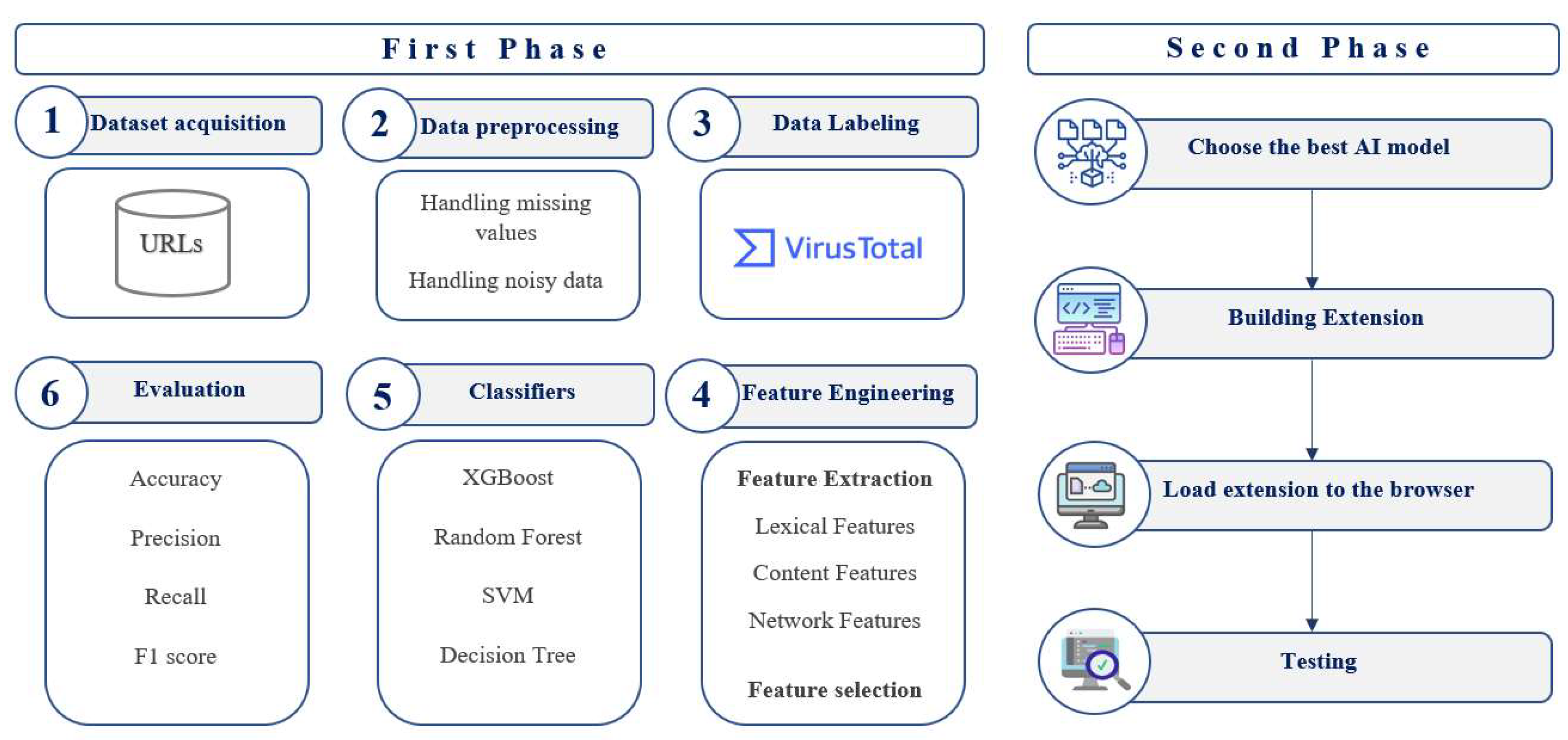
This study uses machine learning (ML) to classify Arabic websites as benign, suspicious, or phishing. As depicted in Figure 1, we followed two main phases to satisfy the study goal.

Figure 1.
Methodology.
In the first phase, the dataset was collected based on the keywords of Google Trends to find the maximum number of phishing and suspicious websites. Google Trends [19] is a service provided by Google that provides public discovery about the trends of people’s search behavior within Google Search. After collecting the keywords, Helium Scraper tool [20] was utilized to collect the URLs. The Helium Scraper tool is manufactured by Helium 10 in Los Angeles, California, United States. The dataset was then cleaned by handling the missing values and the noisy data in the pre-processing step.
The dataset was preprocessed in three steps. First, the data were cleaned by filling in the missing values. Second, noisy data are handled, such as removing non-Arabic web pages, not-found pages, or pages with an internal server error. Third, alphabets were represented as numerical values in the dataset. For instance, we count the lengthy popular keywords instead of using the keyword itself.
The URLs were then classified and labeled as benign, suspicious, or phishing using VirusTotal [21]. This was followed by the feature engineering step, which includes feature extraction and selection. The URL’s lexical, content-based, and network-based features were extracted from the dataset. The most suitable features that enhance the accuracy were selected using the following methods: correlation, hi-square, and ANOVA. Then, we applied four ML classification algorithms: RF, XGBoost, SVM, and DT. Those algorithms were selected based on our previous survey of applying ML techniques to detect malicious URLs [8]. We evaluated the models using four evaluation metrics: accuracy, recall, F1 score, and precision.
The best-performing model was then used to create the website extension. Lastly, we tested the functionality by loading the website extension on the Chrome browser and determining whether a given URL would be correctly classified in a short time.
3.1. Dataset Description
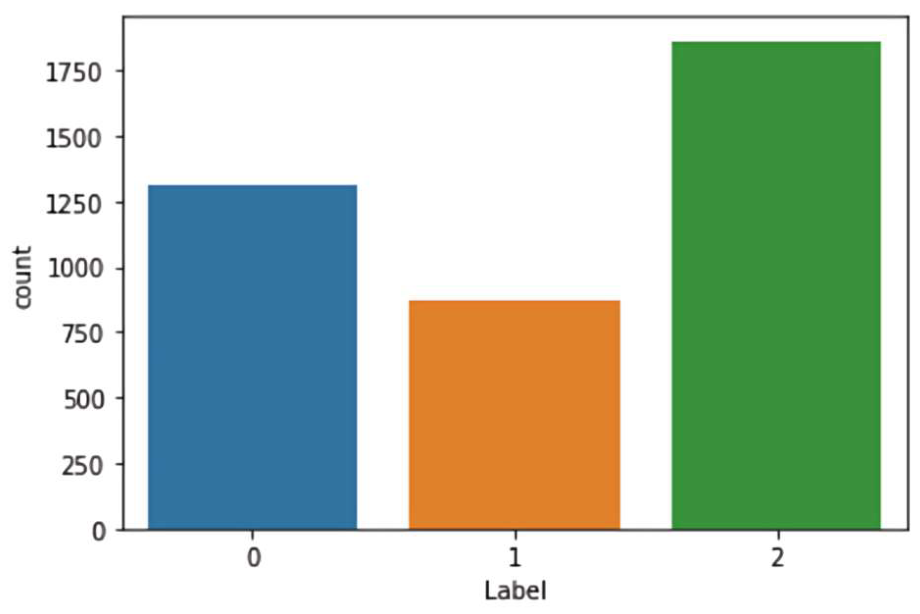
In the beginning, the dataset contained a total of 15,000 URLs, out of which 11,906 URLs were collected using the Helium Scraper tool and 3094 URLs were collected from the ArabicWeb16 dataset [22]. Helium Scraper is a tool that extracts content from websites by identifying target elements and specifying the desired content by typing the wanted keywords in the required language and then applying the extraction rules. In addition, it can export the extracted data in different formats [20]. The URLs were labeled as 12,235 benign, 881 malicious, 220 malware, 761 phishing, 304 spam, and 569 suspicious URLs based on VirusTotal API. The VirusTotal API allows programmatic interaction with VirusTotal through an API Key, which any user can obtain by creating an account with VirusTotal [21]. Furthermore, we noticed a huge difference between the benign class and others. As a result, we combined malware and malicious records to be in one category: phishing and spam records to suspicious. Phishing is a method of acquiring information that can involve malware. The term malware is an umbrella term for an entire range of malicious software [23]. Moreover, suspicious activities can be defined as activities that are out of the ordinary, and spam is any unwanted, unsolicited digital communication sent out in bulk. Because there is a possibility that spam could come from good or bad sources, this behavior is suspicious (e.g., spam emails). After combining malware and malicious records, we changed their labels to phishing and spam records’ labels to suspicious. The benign class was under-sampled into 1313 benign records. Moreover, the other classes consist of 1862 phishing and 873 suspicious, totaling 4048 URLs. Figure 2 below shows the number of records in each class: 0 for benign, 1 for suspicious, and 2 for phishing. Afterward, 17 lexical features, 13 network features, and 9 content features were extracted.
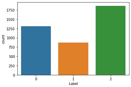
Figure 2.
Dataset records.
3.2. Features Extraction
This section explained the features used: lexical, network, and content. Feature extraction from URLs involves extracting relevant information from the URL to create a structured dataset. This process is essential for URL classification, phishing detection, and web analytics. We can gain valuable insights into the URL’s content, purpose, and potential risks by analyzing features such as the domain name, top-level domain, path, query parameters, and anchor text.
3.2.1. Lexical-Based Features
The lexical features of a URL demonstrated in Figure 3, such as its length, domain name length, special characters, and the presence of “www”, can provide valuable insights into its credibility. Analyzing these elements can assess the URL’s readability, trustworthiness, and relevance to specific topics. For example, a shorter URL with fewer special characters and a recognizable domain name is generally considered more user-friendly and trustworthy. Additionally, the presence of “www” can indicate a commercial or business website. Table 1 shows the features used and explains each feature.

Figure 3.
URL component.

Table 1.
Lexical features.
3.2.2. Network-Based Features
The network features are extracted from the URL component, as in Figure 3. By analyzing these features, we can assess the domain’s stability and trustworthiness. The lifetime and activity of a domain can provide valuable insights into its reliability. Moreover, the remaining days before expiration indicate the domain’s longevity and the owner’s commitment to maintaining it. In addition, a longer lifetime suggests a more established and trusted website. Additionally, the active time of a domain, which refers to the period during which it has been actively registered and used, can reveal its history and potential changes in ownership or purpose.
Table 2 shows the features used and shows whether the feature output needs to be encoded.

Table 2.
Network features.
3.2.3. Content-Based Features
This feature depends on the URL content to extract the necessary information for each feature. Table 3 lists the features we used in the extension. The number of <img> tags indicate the presence and quantity of images, suggesting the informative nature of the website. Counting the <meta> tags provide information about the page’s content, keywords, and description, which can impact search engine rankings and user engagement. Additionally, analyzing the count of repeated and lengthy popular keywords based on Google Trends can reveal the website’s focus and relevance to current trends, influencing its visibility and user interest.

Table 3.
Content-based features.
3.3. Feature Selection
Feature selection is a strategy for selecting a subset of features that contributes more to the prediction variable (URL label) in the dataset. Feature selection aids the effectiveness and efficiency of AI models by reducing time complexity and high data dimensionality. However, irrelevant features can also cause AI models to be misled, resulting in less accuracy [25]. We selected ANOVA, correlation, and chi-square based on their high accuracies in previous studies, such as [26,27]. The methods of the feature selection are discussed below:
- Correlation
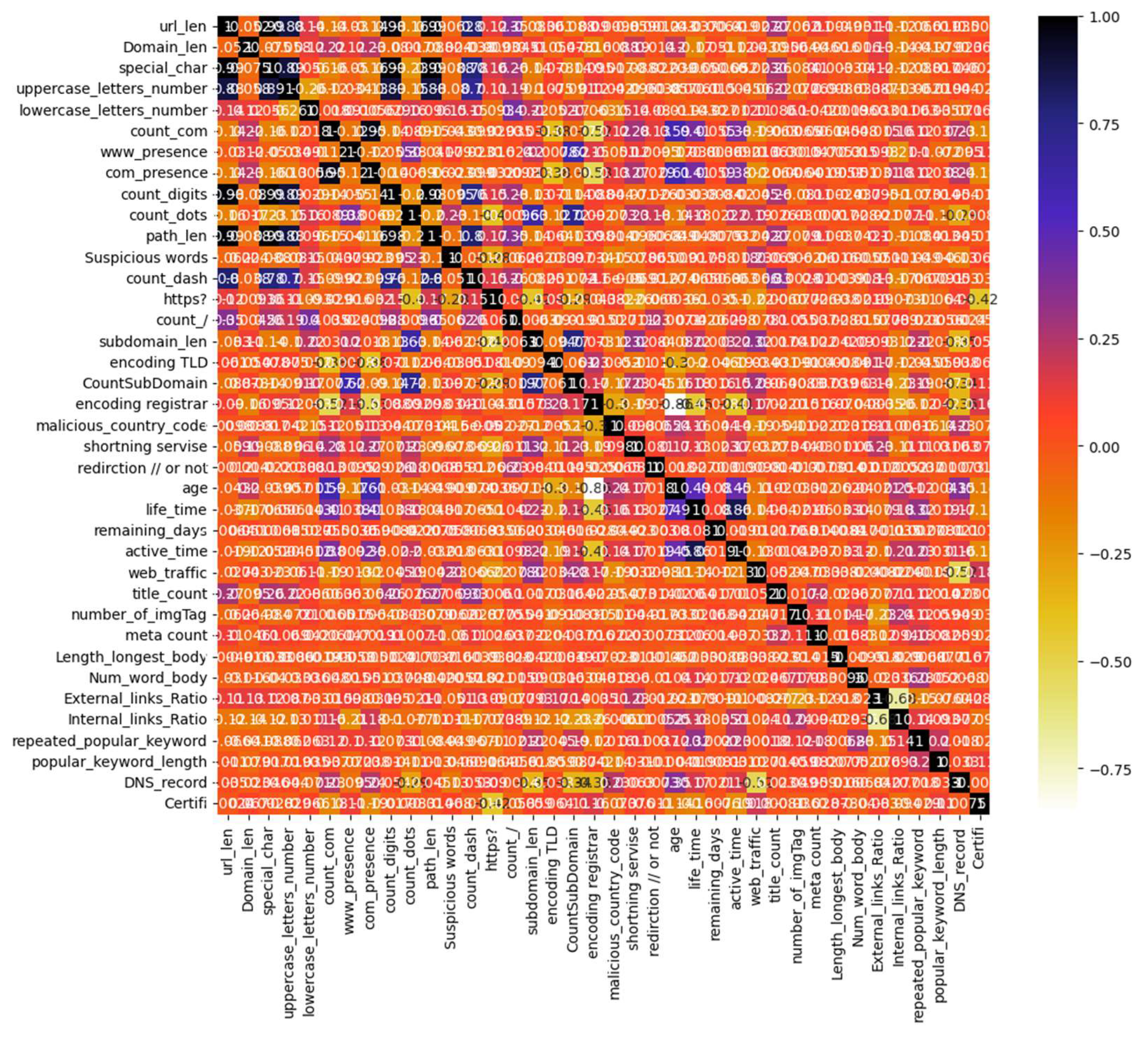
Correlation is a well-known statistical measure that measures the similarity between two features. The correlation coefficient between the two features results in a value that is one if they are linearly dependent and otherwise zero. The correlation approach is used to determine the relationship between the features. There are two basic groups to determine the correlation between two random variables. The first is based on linear correlation, whereas the second is based on information theory. The following formula gives the linear correlation coefficient ‘r’ for a pair of variables (X, Y) [28]. Moreover, in Figure 4, the heatmap of the features shows a strong positive correlation among url_len, special_char, count_digits, and path_len. Moreover, count_com and com_presence are strongly positive correlated to each other.
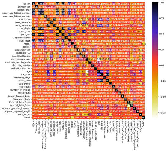
Figure 4.
Attribute correlation heatmap.
- Chi-square
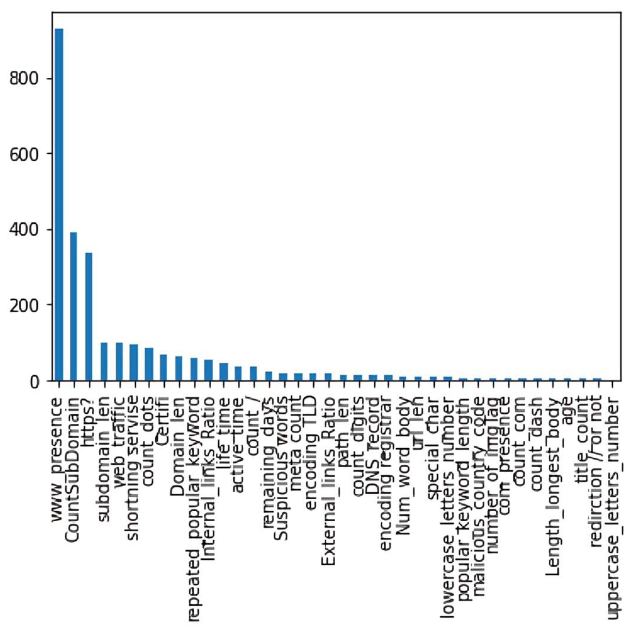
Chi-square is a statistical test used to see if two categorical variables are independent or how closely a sample fits the distribution of a known population. Alternatively, it calculates the distinction between the actual and expected outcomes. For example, consider two variables, O for the observed value and E for the expected value. The following formula can be given: if the chi-square value is large, the feature is more dependent, and the model can be applied to it [29].
Moreover, Figure 5 shows that lifetime, active time, number of words in the body of the page, and remaining days before the domain expire are the top features that contribute to output, while the other features have almost no impact.
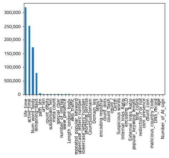
Figure 5.
Feature ranking of chi-square.
- ANOVA
ANOVA is a statistical approach that compares the means of two or more groups that differ considerably. It determines whether there is a significant difference between the means of multiple datasets [30]. The test determines the impact that independent variables have on the dependent variable. Moreover, Figure 6 presents ANOVA feature ranking, which shows that www presence is the feature with the highest p-value, which is irrelevant for predicting the classification of the Arabic websites in our dataset.

Figure 6.
Feature ranking of ANOVA.
Table 4 below shows the feature set selected by each method.

Table 4.
Feature selection techniques and their corresponding features.
ANOVA highlighted features that exhibited distinct mean differences across different URL categories, suggesting their potential importance in classification. Chi-square pinpointed features that demonstrated strong associations with the target variable, indicating a significant correlation between feature values and the target variable. Correlation analysis revealed features that exhibited linear relationships with the class labels, implying a direct influence on classification outcomes.
To determine the most effective feature set for our classification task, we applied a variety of machine-learning models to the datasets resulting from each feature selection technique. By comparing the performance of these models, as measured by accuracy, we identified the feature selection method that consistently yielded the highest classification accuracy, thus revealing the most essential features for precise URL classification.
3.4. Machine Learning Classifiers
This section details the ML classifiers, including RF, XGBoost, DT, and SVM. For all classifiers, we employed an 80–20 split for training and testing the dataset. Additionally, we utilized grid search algorithm to optimize parameters and achieve the highest possible accuracy.
- RF Classifier
RF is a supervised ML method that works based on the ensemble method, which is based on DTs and can handle classification and regression problems.
An ensemble method means an RF algorithm comprises many small DTs called estimators, each of which makes its predictions. The RF method combines the estimators’ predictions for a more precise prediction. For classification problems, the RF output is the class majority voting selects. For regression problems, the output is the mean or average prediction of each tree [31].
When using the RF method to solve regression problems, the mean squared error (MSE) can be used [32]. The formula calculates the distance of each node from the predicted actual value, allowing the choice of the branch that suits the forest the most, and it is given in the following equation:
where X is the number of data points, Yi is the value returned by the DT, and is the value of the data point tested at a particular node. When the RF method is used to solve classification problems, Gini index or information gain (IG) is used. The Gini of each section on a node is calculated using the probability and the class, indicating which branch is more likely to occur. The formula that calculates the Gini index is given in the following equation [32]:
pi represents the relative frequency of the class observed in the dataset, and N represents the number of classes. IG is another measure to choose the appropriate data split based on each feature’s gain. The formula that calculates the IG is given in the following equation [32]:
The hyperparameters and their optimal values for RF are presented in Table 5. The random_state parameter enables us to set a random seed (which is 42) to the random number generation process in the RF, so that, each time we build the model with the same data, we obtain the same one. Moreover, n_estimators represent the number of trees in the forest, which is 1400. The max_features parameter represents the feature number to be considered while determining the optimum split for the tree. If the max_features parameter is set to auto, the tree will use the square root of the feature number as the max_features value. In addition, the max_depth parameter represents the maximum number of levels in each DT, which is 18. The criterion parameter ‘entropy’ represents the function used to measure a split’s quality.

Table 5.
Grid parameters of RF classifier.
- XGBoost Classifier
XGBoost is an ensemble technique based on DTs, a type of gradient boosting. It is a supervised learning method based on function approximation through the optimization of specific loss functions and the application of various regularization methods, and it supports parallel processing, handles missing values, offers cache optimization, takes care of outliers to some extent, and has inbuilt cross-validation. XGBoost can be utilized to solve regression and classification problems. The algorithm combines the estimates of a group of smaller, weaker models to predict a target variable accurately. The general equation of the algorithm consists of two parts, training loss and regularization term as follows [33]:
where L represents the training loss function, and represents the regularization parameters. The training loss measures determine how well a model predicts the training data, and MSE is a common choice of L. Regularization helps prevent the problem of overfitting by controlling the model’s complexity [33].
The hyperparameters and their optimal values for XGBoost are presented in Table 6, where the n_estimator value is 600, the max_depth value is 22, and the gamma parameter specifies the least loss reduction required to make a split, which is 0.5. Furthermore, the learning_rate parameter value is 0.09, representing the weights assigned to the tree in the next iteration. The colsample_bytree parameter value is 0.7, representing the fraction of columns to be randomly sampled for each tree. Moreover, the booster parameter selects the type of model to run at each iteration, and the value ‘gbtree’ means that the model is tree-based. The cv parameter with the value 5 determines the cross-validation splitting strategy.

Table 6.
Grid parameters of XGBoost classifier.
- DT Classifier
DT is a supervised learning technique that can be used for regression and classification problems [34]. Moreover, DT classifier is constructed as a tree-like structure that represents all possible results of a decision based on defined conditions. Furthermore, DT comprises three essential elements: decision nodes (internal nodes), branches, and leaf nodes. The data are branched into two distinct categories, with each internal node representing an attribute. This is repeated until a class label, represented by a leaf, is reached.
Table 7 presents the hyperparameters and their optimal values for DT. The max_depth is 30, the max_features is auto, and the criterion value is entropy. The ccp_alpha parameter, with a value of 0.001, refers to the cost complexity parameter that provides another option for controlling the tree size. The greater the value of ccp_alpha, the more nodes are pruned.

Table 7.
Grid parameters of DT classifier.
- SVM Classifier
SVM is a supervised learning algorithm that can solve classification and regression problems. It utilizes a dataset in which the input samples are separated into two classes with labels 0 or 1. The algorithm aims to find a line or plane, known as a hyperplane, that will most efficiently divide the two classes [35].
B0 + (B1 × X1) + (B2 × X2) = 0
The above equation represents the hyperplane equation which can be used to find whether the new example falls in class 0 or 1 side. The coefficients (B1 and B2) give the slope of the line, and the algorithm calculates the intercept (B0). X1 and X2 are the two input data points [35].
The hyperparameters and their optimal values for SVM are presented in Table 8. The first parameter is gamma, with a value of 0.01, which sets the distance of influence of a single training point. Near points will affect classification if the gamma value is high. In other words, the data points must be close to each other to be considered in the same class. However, if the gamma value is low, distant data points will influence the classification, which results in more data points being grouped. The second parameter is the kernel function parameter, with the value of rbf, which is used to transform non-linearly separable data into linearly separable one using the radial basis function (RBF). The third parameter is the C parameter, which defines how much misclassification of the training data is permitted in the model. If the C value is small, the decision boundary with a large margin will be chosen. However, if the C value is small, the SVM classifier attempts to reduce the number of misclassified ones, resulting in a decision boundary with a narrower margin [36].

Table 8.
Grid parameters of SVM classifier.
3.5. Building Extension
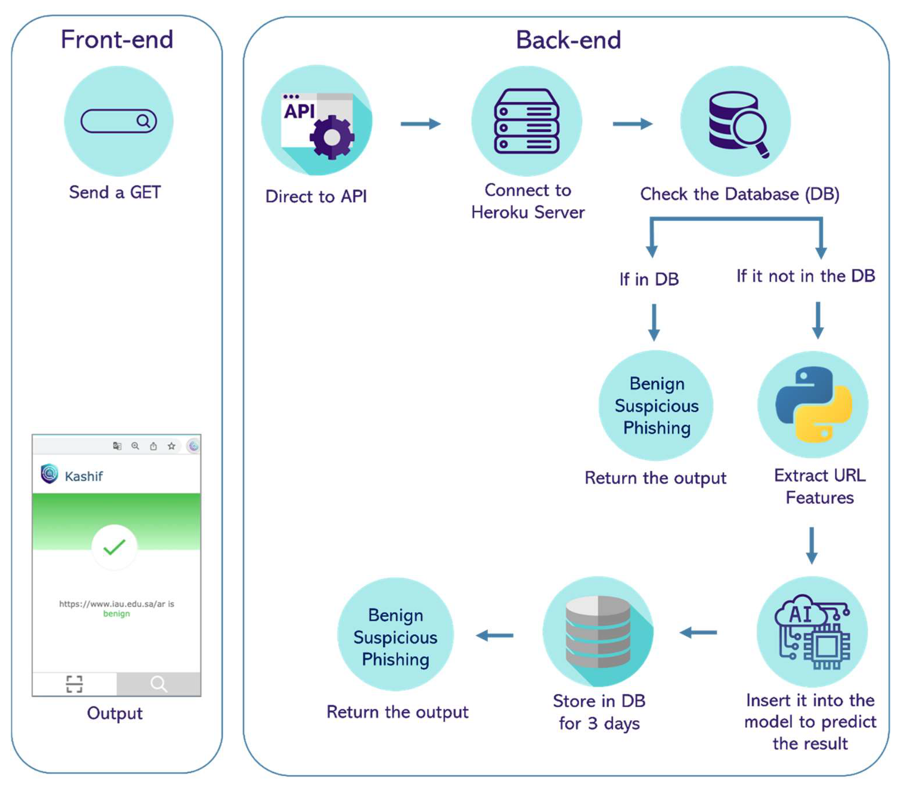
Google Chrome is the most commonly used browser in the world. It is a user-friendly interface that raises the standard for modern browser design. Furthermore, to enable proper functioning, we divided the work into two parts: the frontend and the backend. The frontend is the part with which a user interacts, whereas the backend is the framework that enables this interaction. The frontend includes two interfaces: a scanning interface that obtains the URL and processes it, then returns the label of the currently opened page, and the second is a search interface that enables users to enter any URL and returns the result.
The backend is the backbone of the system that is based on the Django framework, Django Rest API, Postgres SQL Database [37], and Heroku Server [38]. Moreover, it includes the feature extraction function (its result is the input of the trained model). In addition, it includes the trained ML model to predict the URL label. Django is a Python full-stack web framework that allows for the rapid building of safe and maintained websites. It is free and open-source for users [39]. The REST APIs define what requests can be made to a component, how to make them (by GET, POST, etc.), and their expected responses.
In Figure 7, the entire process of Kashif is presented. The user can search for a specific URL, or the current page’s URL will be sent to the Django framework (backend). After that, the workflow of the Kashif extension requires the users to be able to access a database in terms of obtaining a result from an existing URL with its label or saving a new result that consists of a URL with its corresponding label through the REST API that will communicate with the users’ input in the frontend (obtain the URL from the current page or the search page) by the GET method.
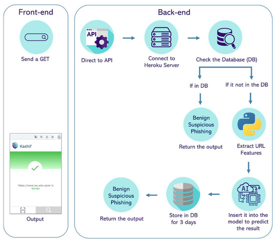
Figure 7.
Backend and frontend structure.
Therefore, the URL will be searched in the database, and, if the same URL is found, the result will be displayed to the user. If not, the features of the URL will be extracted to send the output to the ML model to predict the label of the URL, and the result will be saved in the database. At the same time, the result will be sent back to the user.
4. Results and Discussion
This section discussed the models’ performance. We have recorded the accuracy for each classifier with each feature selection technique, as in Table 9.

Table 9.
Model performance (accuracy).
Overall, the accuracies without using the feature selection technique are higher than the others, especially in XGBoost, RF, and DT. Moreover, XGBoost and RF have almost the same results for each feature selection technique, and the SVM and DT have almost the same results for each feature selection. XGBoost and RF outperform SVM and DT because both have the built-in capability to handle imbalanced datasets [40,41], and they have used the concept of the ensemble method. Ensemble methods are an ML technique that combines several classifiers to produce one optimal predictive model. XGBoost has a boosting nature that uses ensemble techniques. Therefore, XGBoost inherits the ensemble techniques. The RF is the ensemble of the DTs, and it builds a forest of many random DTs.
Moreover, algorithms work differently. For example, the DT classifier is built as a tree-like structure that reflects all possible outcomes of a decision depending on specified conditions, whereas the SVM uses a separator line between the categories, and the data are transformed to draw the separator, as in Figure 8.
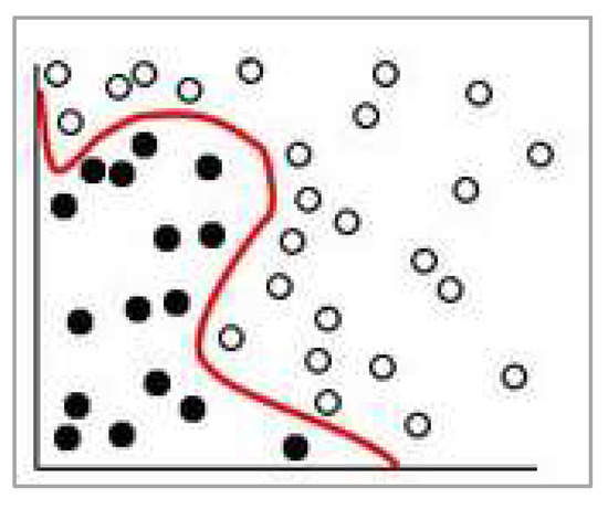
Figure 8.
The separator line in the SVM.
To set up the model that was deployed in the Kashif extension, we took the decision based on three standards: 1—high accuracy, 2—containing content-based features that include an analysis of the Arabic text in the web page, 3—maintaining the speed of extraction and prediction of the result. The first choice was XGBoost model, which achieved the highest accuracy at 95.55% without using a feature selection method. However, extracting and predicting data can be time-consuming, which is an issue because users generally expect the system to work quickly. The second choice is XGBoost with chi-square, which achieved an accuracy of 92.71%. However, the chi-square method did not choose the content features that matter about the Arabic content; it included the content features included in Table 3, such as the meta count, which does not contain any Arabic-content analysis. In other words, the chi-square method did not choose features that analyze Arabic words, such as counting lengthy popular keywords and counting repeated popular keywords inside the body tag. The third choice was to manually add two features that met our standards to the chi-square set since it has the highest accuracies among the other methods and fewer sets of features.
The features added to it are the count of lengthy popular keywords and the count of repeated popular keywords (based on Google Trends) inside the body tag. Counting repeated popular keywords and lengthy popular keywords within the body of Arabic websites, based on Google Trends data, is significant. These features were not commonly used before for Arabic websites, as they provide insights into the relevance and engagement of content. Website owners can tailor their content to match user search intent and improve search engine rankings by analyzing the keyword frequency and length based on trending topics.
Then, we compared the results and found that the RF model with the selected features by chi-square and two more features achieved the highest accuracy of 92.96%. After we chose the model, we applied other evaluation metrics to check its performance, as in Table 10.

Table 10.
Evaluation metrics for the chosen model.
The confusion matrix is an ML categorization performance metric. It is a table with four or more (depending on the number of classes) different predicted and actual values. The confusion matrix gives the amount of (mis)classifications for each class, and it uses TP, TN, FP, and FN, where they stand for the following [42]:
- True Positive: the prediction is positive, and it is true;
- True Negative: the prediction is negative, and it is true;
- False Positive: the prediction is positive, and it is false;
- False Negative: the prediction is negative, and it is false.
The next Figure 9 shows the confusion matrix for the chosen model:
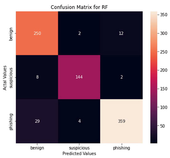
Figure 9.
Confusion matrix for the chosen model.
- Our model predicted 250 labels that are not benign, and they actually are not benign;
- Our model predicted 8 that are not suspicious, and they actually are suspicious;
- Our model predicted 29 that are not phishing, and they actually are not phishing;
- Our model predicted 2 benign and they actually are not benign;
- Our model predicted 144 suspicious, and they actually are suspicious;
- Our model predicted 4 phishing, and they actually are not phishing;
- Our model predicted 12 labels that are not benign, and they actually are not benign;
- Our model predicted 2 labels that are not suspicious, and they actually are suspicious;
- Our model predicted 359 labels that are not phishing, and they actually are not phishing.
5. Conclusions
In this paper, we investigated the security of Arabic websites by constructing a detection tool that analyzes Arabic content using artificial intelligence approaches. We created four distinct ML models, XGB, RF, DT, and SVM, with different feature extraction and selection techniques. The work was embedded in a Chrome extension based on an RF model using the features selected using the chi-square approach; this developed tool reached an accuracy of 92.96%. Our extension will enable users to determine whether a web page is phishing, suspicious, or benign. In the future, we plan to increase our dataset size to allow the ML models to learn from different URL examples. Moreover, we will create different ML models that adopt the concept of continuous AI to refresh our models on a specific schedule, for example, every three months or when an event happens, like a drop in the accuracy or changes in the features’ importance. Since we only employed an ML model, we plan to try and compare different DL models such as the CNN, ANN, and LSTM. Furthermore, releasing an Arabic version of the Kashif extension and other versions of the Kashif that could operate on different web browsers such as Safari and Mozilla Firefox. In addition, we will enhance the users’ protection by preventing the loading of phishing web pages.
Author Contributions
Conceptualization, M.A.; methodology, M.A., A.A.A., R.M.A.M., F.A., H.S.A., S.A.A., M.A.-H., H.T.A. and N.K.A.; software, H.S.A., S.A.A., M.A.-H., H.T.A. and N.K.A.; formal analysis, H.S.A., S.A.A., M.A.-H., H.T.A. and N.K.A.; validation, M.A., A.A.A., R.M.A.M., F.A., H.S.A., S.A.A., M.A.-H., H.T.A. and N.K.A.; investigation, M.A., A.A.A., R.M.A.M., F.A., H.S.A., S.A.A., M.A.-H., H.T.A. and N.K.A.; resources, H.S.A., S.A.A., M.A.-H., H.T.A. and N.K.A.; data curation, H.S.A., S.A.A., M.A.-H., H.T.A. and N.K.A.; writing—original draft preparation, H.S.A., S.A.A., M.A.-H., H.T.A. and N.K.A.; writing—review and editing, M.A. and H.S.A.; visualization, H.S.A., S.A.A., M.A.-H., H.T.A. and N.K.A.; supervision, M.A. and A.A.A.; project administration, M.A. and A.A.A.; funding acquisition, F.A. All authors have read and agreed to the published version of the manuscript.
Funding
This research was funded by the SAUDI ARAMCO Cybersecurity Chair at Imam Abdulrahman Bin Faisal University (IAU).
Institutional Review Board Statement
Not applicable.
Informed Consent Statement
Not applicable.
Data Availability Statement
The dataset is not available online right now. For any inquiries, contact the authors.
Acknowledgments
The authors thank the SAUDI ARAMCO Cybersecurity Chair at Imam Abdulrahman Bin Faisal University for funding this project.
Conflicts of Interest
The authors declare that there are no conflicts of interest regarding the publication of this paper.
References
- Aljabri, M.; Aljameel, S.S.; Mohammad, R.M.A.; Almotiri, S.H.; Mirza, S.; Anis, F.M.; Aboulnour, M.; Alomari, D.M.; Alhamed, D.H.; Altamimi, H.S. Intelligent Techniques for Detecting Network Attacks: Review and Research Directions. Sensors 2021, 21, 7070. [Google Scholar] [CrossRef] [PubMed]
- Aljabri, M.; Aldossary, M.; Al-Homeed, N.; Alhetelah, B.; Althubiany, M.; Alotaibi, O.; Alsaqer, S. Testing and Exploiting Tools to Improve OWASP Top Ten Security Vulnerabilities Detection. In Proceedings of the 2022 14th International Conference on Computational Intelligence and Communication Networks (CICN), Al-Khobar, Saudi Arabia, 4–6 December 2022; pp. 797–803. [Google Scholar] [CrossRef]
- Aljabri, M.; Mirza, S. Phishing Attacks Detection using Machine Learning and Deep Learning Models. In Proceedings of the 2022 7th International Conference on Data Science and Machine Learning Applications (CDMA), Riyadh, Saudi Arabia, 1–3 March 2022; pp. 175–180. [Google Scholar] [CrossRef]
- Alzahrani, R.A.; Aljabri, M. AI-Based Techniques for Ad Click Fraud Detection and Prevention: Review and Research Directions. J. Sens. Actuator Netw. 2023, 12, 4. [Google Scholar] [CrossRef]
- Aljabri, M.; Zagrouba, R.; Shaahid, A.; Alnasser, F.; Saleh, A.; Alomari, D.M. Machine learning-based social media bot detection: A comprehensive literature review. Soc. Netw. Anal. Min. 2023, 13, 20. [Google Scholar] [CrossRef]
- Nguyen, G.; Dlugolinsky, S.; Bobák, M.; Tran, V.; López García, Á.; Heredia, I.; Malík, P.; Hluchý, L. Machine Learning and Deep Learning frameworks and libraries for large-scale data mining: A survey. Artif. Intell. Rev. 2019, 52, 77–124. [Google Scholar] [CrossRef]
- Aljabri, M.; Alhaidari, F.; Mohammad, R.M.A.; Mirza, S.; Alhamed, D.H.; Altamimi, H.S.; Chrouf, S.M.B. An Assessment of Lexical, Network, and Content-Based Features for Detecting Malicious URLs Using Machine Learning and Deep Learning Models. Comput. Intell. Neurosci. 2022, 2022, 3241216. [Google Scholar] [CrossRef] [PubMed]
- Aljabri, M.; Altamimi, H.S.; Albelali, S.A.; Al-Harbi, M.; Alhuraib, H.T.; Alotaibi, N.K.; Alahmadi, A.A.; Alhaidari, F.; Mohammad, R.M.A.; Salah, K. Detecting Malicious URLs Using Machine Learning Techniques: Review and Research Directions. IEEE Access 2022, 10, 121395–121417. [Google Scholar] [CrossRef]
- Gurjar, N.S.; Sudheendra, S.R.; Kumar, C.S.; Krishnaveni, K.S. WebSecAsst—A Machine Learning based Chrome Extension. In Proceedings of the 6th International Conference on Communication and Electronics Systems, ICCES 2021, Coimbatre, India, 8–10 July 2021; pp. 1631–1635. [Google Scholar] [CrossRef]
- Sigillito, V. UCI Machine Learning Repository: Ionosphere Data Set. UCI Machine Learning Repository: Ionosphere Data Set. Available online: https://archive.ics.uci.edu/ml/datasets/phishing+websites (accessed on 4 July 2022).
- Shivangi, S.; Debnath, P.; Saieevan, K.; Annapurna, D. Chrome Extension for Malicious URLs detection in Social Media Applications Using Artificial Neural Networks and Long Short Term Memory Networks. In Proceedings of the 2018 International Conference on Advances in Computing, Communications and Informatics, ICACCI 2018, Bangalore, India, 19–22 September 2018; Institute of Electrical and Electronics Engineers Inc.: Piscataway, NJ, USA, 2018; pp. 1993–1997. [Google Scholar] [CrossRef]
- Common Crawl. “Common Crawl”. Available online: http://commoncrawl.org/ (accessed on 4 December 2021).
- Esler, J. PhishTank-Join the Fight against Phishing. Available online: https://www.phishtank.com (accessed on 12 January 2022).
- Syafiq Rohmat Rose, M.A.; Basir, N.; Nabila Rafie Heng, N.F.; Juana Mohd Zaizi, N.; Saudi, M.M. Phishing Detection and Prevention using Chrome Extension. In Proceedings of the 2022 10th International Symposium on Digital Forensics and Security (ISDFS), Istanbul, Turkey, 6–7 June 2022; pp. 1–6. [Google Scholar] [CrossRef]
- Pagadala, K. Detecting Phishing sites Without Visiting them. arXiv 2022, arXiv:2205.05121. [Google Scholar] [CrossRef]
- Majestic Million. Available online: https://majestic.com/reports/majestic-million (accessed on 16 July 2022).
- Kumar Kureel, V.; Maurya, S.; Shaikh, A.; Tiwari, S.; Nagmote, S. PHISHING WEBSITE DETECTION USING MACHINE LEARNING. Int. J. Res. Publ. Rev. 2022, 3, 2657–2663. [Google Scholar]
- Alsaleh, M.; Alarifi, A. Analysis of web spam for non-English content: Toward more effective language-based classifiers. PLoS ONE 2016, 11, e0164383. [Google Scholar] [CrossRef]
- Google Trends. Available online: https://trends.google.com/trends/trendingsearches/daily?geo=SA (accessed on 19 February 2023).
- Web Scraper|Helium Scraper. Available online: https://www.heliumscraper.com/eng/ (accessed on 21 November 2021).
- VirusTotal-Home. Available online: https://www.virustotal.com/gui/home/url (accessed on 19 February 2023).
- Suwaileh, R.; Kutlu, M.; Fathima, N.; Lease, M. ArabicWeb16: A New Crawl for Today’s Arabic Web. In Proceedings of the 39th International ACM SIGIR Conference on Research and Development in Information Retrieval, Pisa, Italy, 17–21 July 2016. [Google Scholar] [CrossRef]
- Malware, Phishing, Spyware and Viruses-What’s the Difference?-PCS. Available online: https://www.pcs-systems.com/different-cyber-threats/ (accessed on 11 May 2022).
- Google Trends. Available online: https://trends.google.com/trends/?geo=SA (accessed on 21 November 2021).
- Feature Selection Techniques in Machine Learning with Python|by Rahil Shaikh|Towards Data Science. Available online: https://towardsdatascience.com/feature-selection-techniques-in-machine-learning-with-python-f24e7da3f36e (accessed on 20 November 2021).
- Al-Kabi, M.N.; Wahsheh, H.A.; Alsmadi, I.M. OLAWSDS: An Online Arabic Web Spam Detection System. J. Adv. Comput. Sci. Appl. 2014, 5, 105–110. [Google Scholar]
- Janet, B.; Kumar, R.J.A. Malicious URL Detection: A Comparative Study. In Proceedings of the International Conference on Artificial Intelligence and Smart Systems, ICAIS 2021, Coimbatore, India, 25–27 March 2021; pp. 1147–1151. [Google Scholar] [CrossRef]
- Blessie, E.C.; Karthikeyan, E. Sigmis: A feature selection algorithm using correlation based method. J. Algorithm Comput. Technol. 2012, 6, 385–394. [Google Scholar] [CrossRef]
- Franke, T.M.; Ho, T.; Christie, C.A. The Chi-Square Test: Often Used and More Often Misinterpreted. Am. J. Eval. 2011, 33, 448–458. [Google Scholar] [CrossRef]
- Shaharum, S.M.; Sundaraj, K.; Helmy, K. Performance analysis of feature selection method using anova for automatic wheeze detection. J. Teknol. 2015, 77, 43–47. [Google Scholar] [CrossRef]
- IBM Cloud Education. What Is Random Forest? Available online: https://www.ibm.com/cloud/learn/random-forest (accessed on 20 February 2022).
- Schott, M. Random Forest Algorithm for Machine Learning. Capital One Tech. Available online: https://medium.com/capital-one-tech/random-forest-algorithm-for-machine-learning-c4b2c8cc9feb (accessed on 6 May 2022).
- Introduction to Boosted Trees—Xgboost 1.6.0 Documentation. Available online: https://xgboost.readthedocs.io/en/stable/tutorials/model.html (accessed on 6 May 2022).
- Sahingoz, O.K.; Buber, E.; Demir, O.; Diri, B. Machine learning based phishing detection from URLs. Expert Syst. Appl. 2019, 117, 345–357. [Google Scholar] [CrossRef]
- Desai, A.; Jatakia, J.; Naik, R.; Raul, N. Malicious web content detection using machine leaning. In Proceedings of the RTEICT 2017—2nd IEEE International Conference on Recent Trends in Electronics, Information and Communication Technology, Bangalore, India, 19–20 May 2017; pp. 1432–1436. [Google Scholar] [CrossRef]
- Hyperparameter Tuning for Support Vector Machines—C and Gamma Parameters|by Soner Yıldırım|towards Data Science. Available online: https://towardsdatascience.com/hyperparameter-tuning-for-support-vector-machines-c-and-gamma-parameters-6a5097416167 (accessed on 15 May 2022).
- What Is PostgreSQL. Available online: https://www.postgresqltutorial.com/postgresql-getting-started/what-is-postgresql/ (accessed on 7 May 2022).
- About Heroku|Heroku. Available online: https://www.heroku.com/about (accessed on 7 May 2022).
- Django Introduction-Learn Web Development|MDN. Available online: https://developer.mozilla.org/en-US/docs/Learn/Server-side/Django/Introduction (accessed on 14 April 2022).
- Using Random Forest to Learn Imbalanced Data. Available online: https://www.researchgate.net/publication/254196943_Using_Random_Forest_to_Learn_Imbalanced_Data (accessed on 12 May 2022).
- How to Configure XGBoost for Imbalanced Classification. Available online: https://machinelearningmastery.com/xgboost-for-imbalanced-classification/ (accessed on 12 May 2022).
- Krüger, F. Activity, Context, and Plan Recognition with Computational Causal Behaviour Models. ResearchGate. Available online: https://www.researchgate.net/figure/Confusion-matrix-for-multi-class-classification-The-confusion-matrix-of-a_fig7_314116591 (accessed on 13 May 2022).
Disclaimer/Publisher’s Note: The statements, opinions and data contained in all publications are solely those of the individual author(s) and contributor(s) and not of MDPI and/or the editor(s). MDPI and/or the editor(s) disclaim responsibility for any injury to people or property resulting from any ideas, methods, instructions or products referred to in the content. |
© 2024 by the authors. Licensee MDPI, Basel, Switzerland. This article is an open access article distributed under the terms and conditions of the Creative Commons Attribution (CC BY) license (https://creativecommons.org/licenses/by/4.0/).

