
Calculation of Maximum Permissible Load of Underground Power Cables–Numerical Approach for Systems with Stabilized Backfill


Abstract
:1. Introduction
1.1. General Description of the Topic
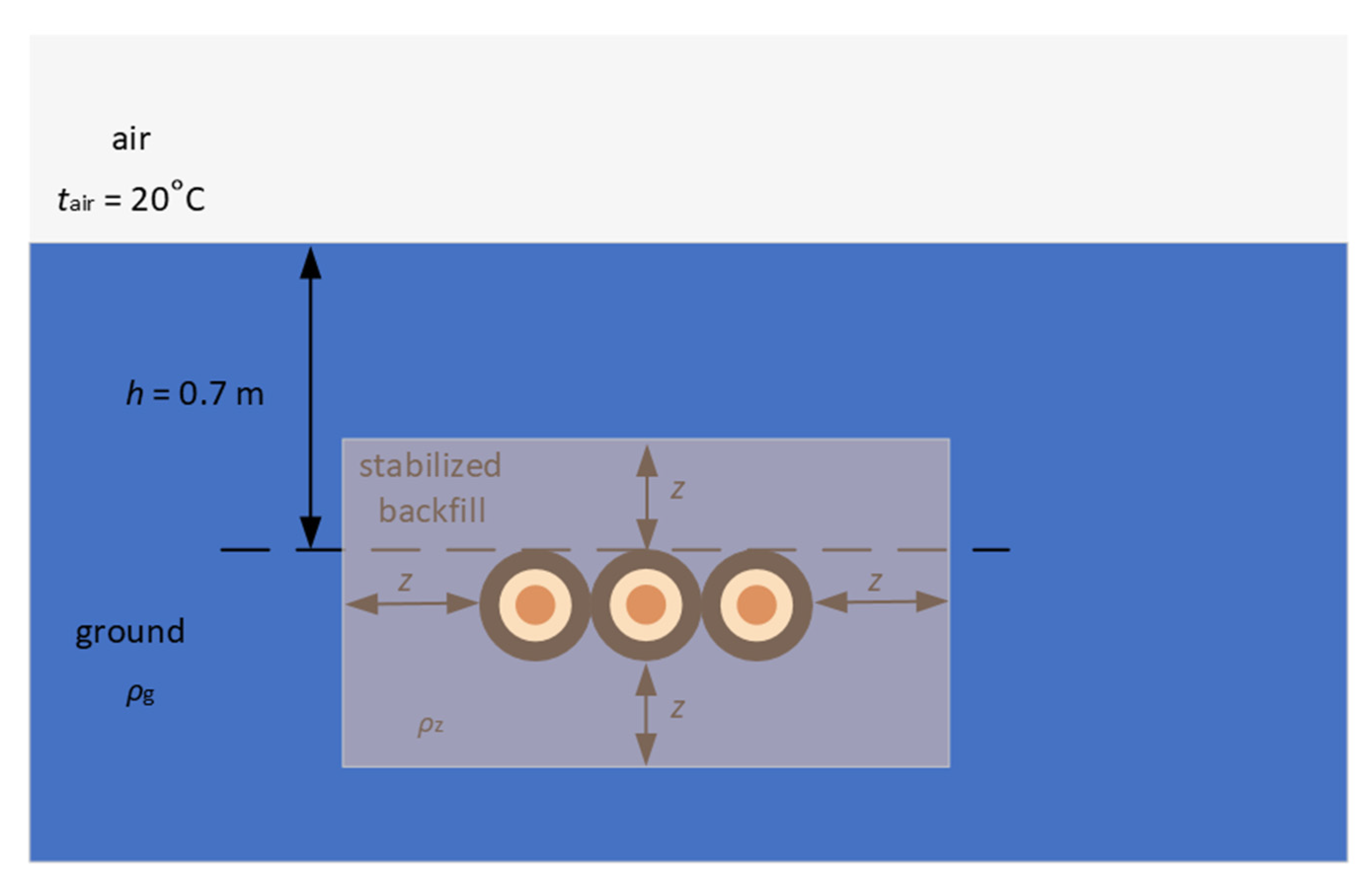
1.2. The Issue of Cable Placement in Stabilized Backfill
2. Materials and Methods
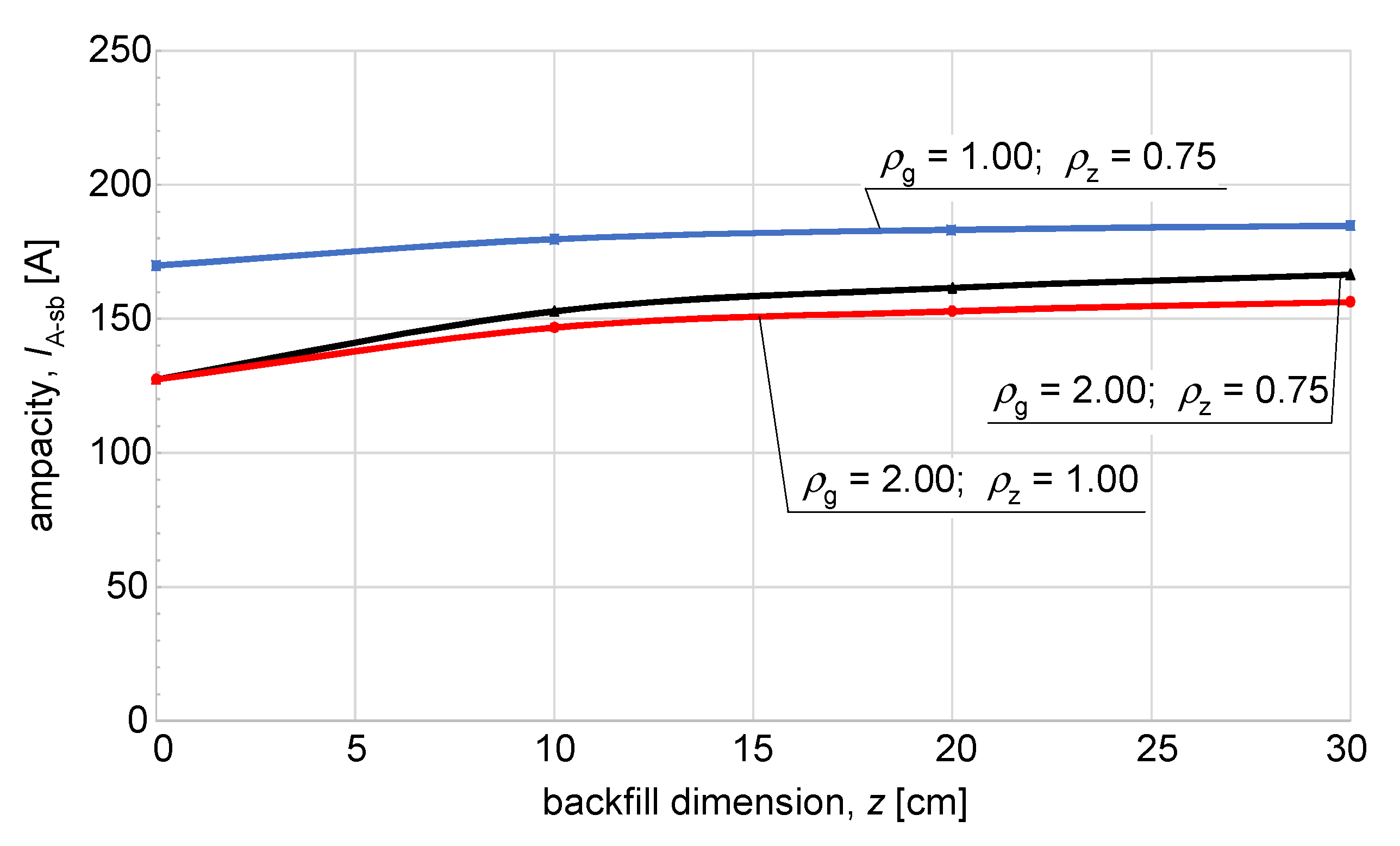
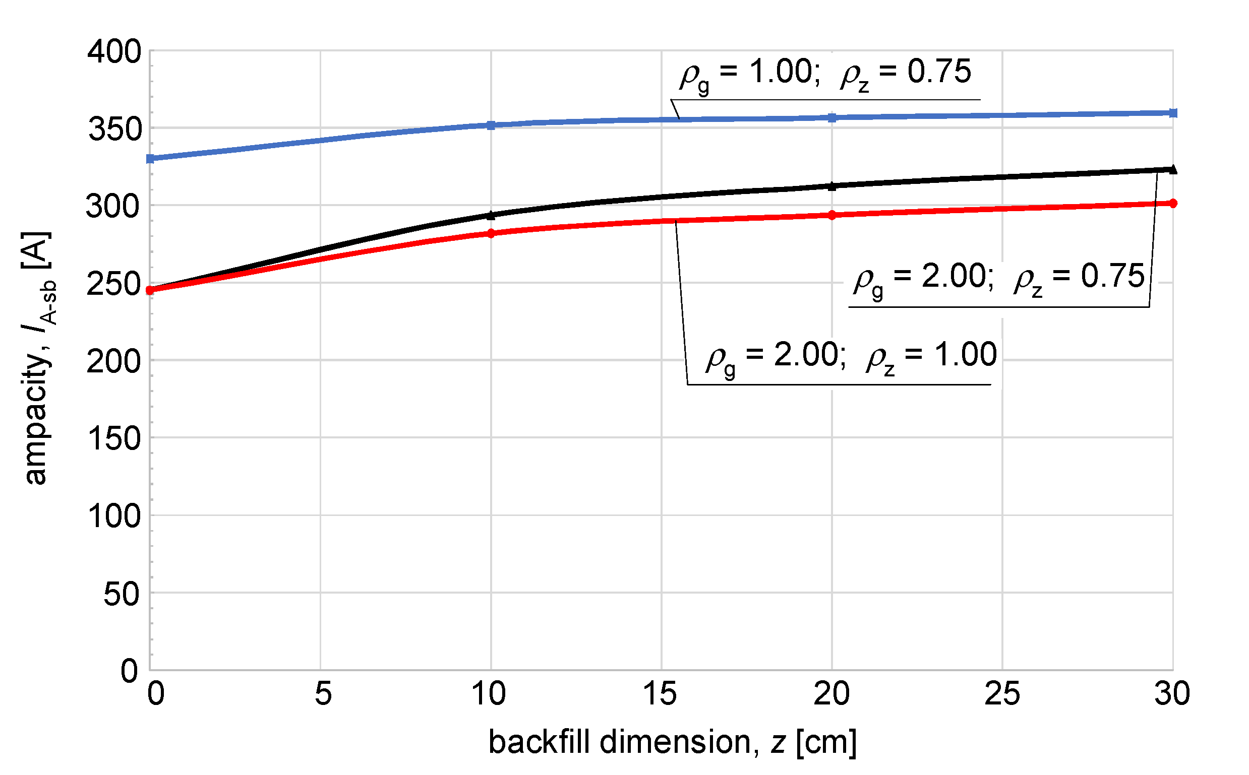
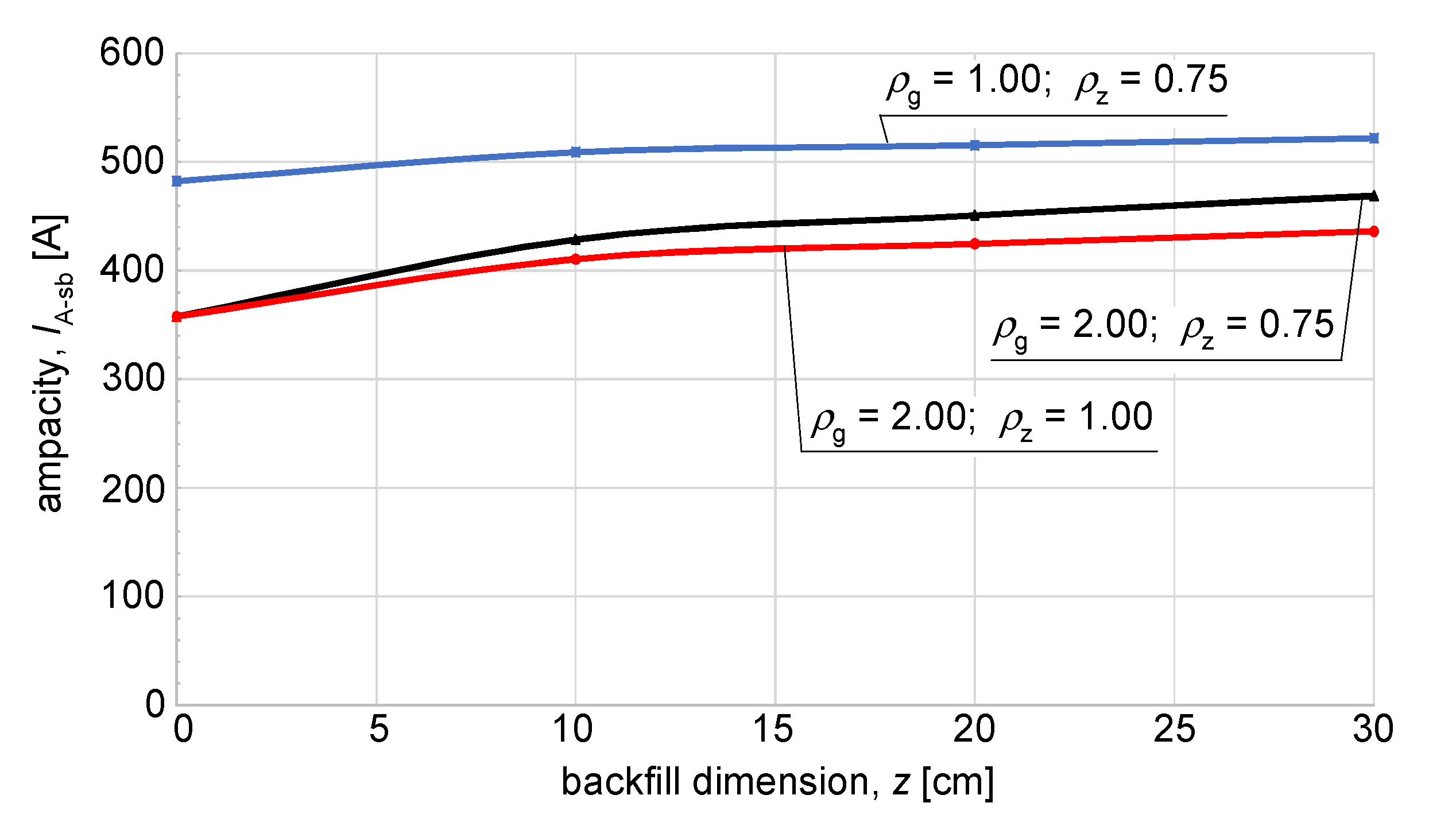
3. Results and Discussion
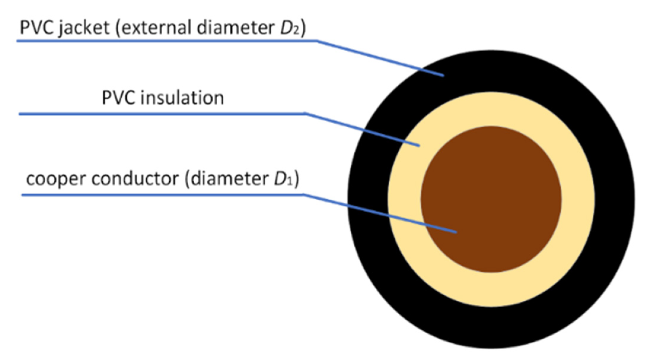
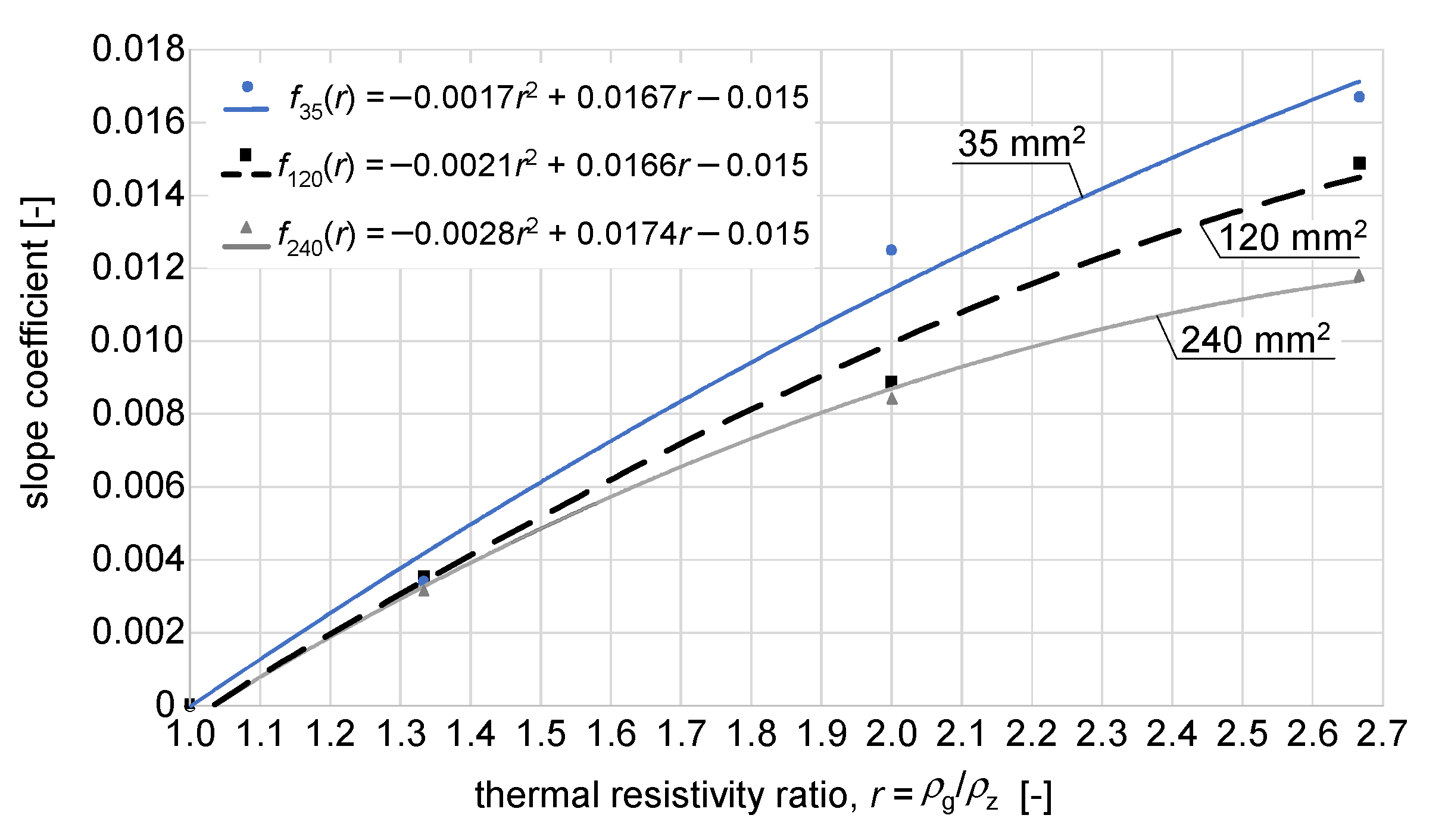
- cross-section of cable cores: , [mm2];
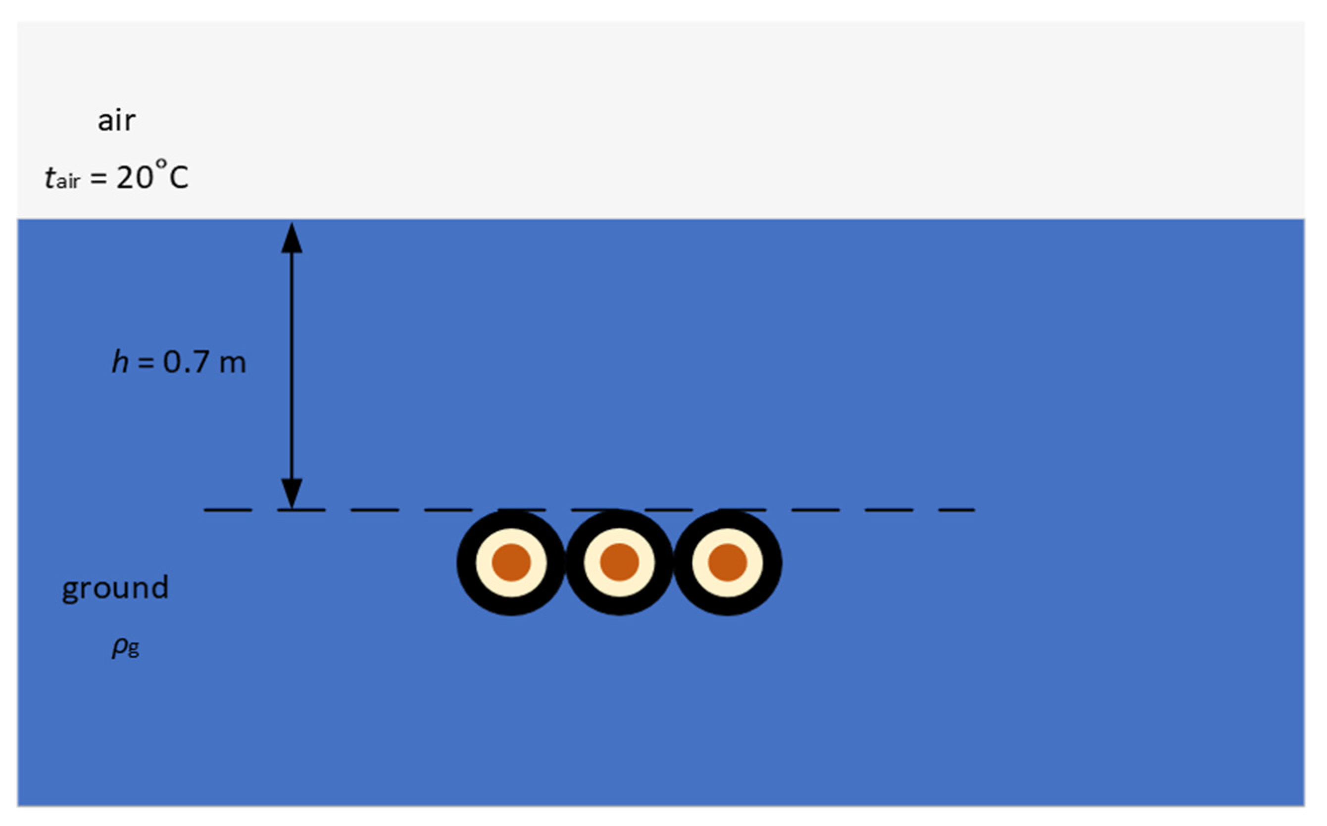
- native soil thermal resistivity: , [(K∙m)/W];
- stabilized backfill thermal resistivity: , [(K∙m)/W];
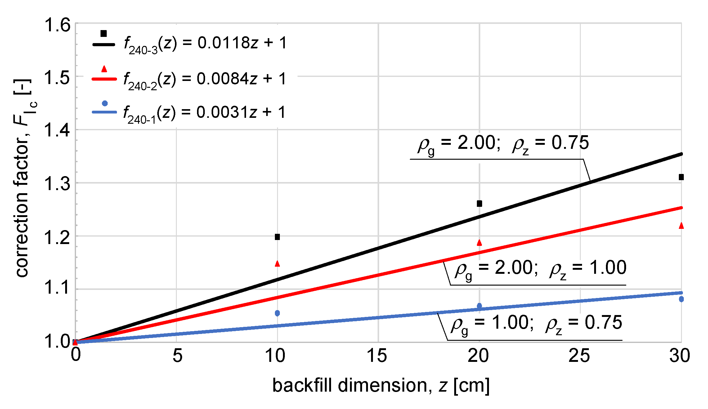
- thermal resistivity ratio: , [-];
- stabilized backfill dimension: , [cm].
4. Conclusions
Author Contributions
Funding
Institutional Review Board Statement
Informed Consent Statement
Data Availability Statement
Conflicts of Interest
References
- Kopsidas, K. A Power System Reliability Framework Considering Soil Drying-Out Effect on Underground Cables. IEEE Trans. Power Syst. 2023, 39, 4783–4794. [Google Scholar] [CrossRef]
- Kornatka, M. Analysis of the exploitation failure rate in Polish MV networks. Eksploat. I Niezawodn. Maint. Reliab. 2018, 20, 413–419. [Google Scholar] [CrossRef]
- Szultka, S.; Czapp, S.; Tomaszewski, A. Impact of thermal backfill parameters on current-carrying capacity of power cables installed in the ground. Bull. Pol. Acad. Sci. Tech. Sci. 2023, 71, 145565. [Google Scholar] [CrossRef]
- Das Gupta, S.; Al-Musawi, M.J. Reliability optimization in cable system design using a fuzzy uniform-cost algorithm. IEEE Trans. Reliab. 1988, 37, 75–80. [Google Scholar] [CrossRef]
- Radakovic, Z.R.; Jovanovic, M.V.; Milosevic, V.M.; Ilic, N.M. Application of Earthing Backfill Materials in Desert Soil Conditions. IEEE Trans. Ind. Appl. 2015, 51, 5288–5297. [Google Scholar] [CrossRef]
- Al-Dulaimi, A.A.; Güneşer, M.T.; Hameed, A.A. Investigation of Thermal Modeling for Underground Cable Ampacity Under Different Conditions of Distances and Depths. In Proceedings of the 5th International Symposium on Multidisciplinary Studies and Innovative Technologies (ISMSIT), Ankara, Turkey, 21–23 October 2021; pp. 654–659. [Google Scholar] [CrossRef]
- Gouda, O.E.; El Dein, A.Z.; Amer, G.M. The effect of the artificial backfill materials on the ampacity of the under-ground cables. In Proceedings of the 7th International Multi-Conference on Systems, Signals and Devices, Amman, Jordan, 27–30 June 2010; pp. 1–6. [Google Scholar] [CrossRef]
- Cichy, A.; Sakowicz, B.; Kaminski, M. Economic Optimization of an Underground Power Cable Installation. IEEE Trans. Power Deliv. 2018, 33, 1124–1133. [Google Scholar] [CrossRef]
- Eckhardt, M.; Pham, H.; Schedel, M.; Sass, I. Investigation of Fluidized Backfill Materials for Optimized Bedding of Buried Power Cables. In Proceedings of the EGU General Assembly 2021, Göttingen, Germany, 19–30 April 2021. EGU21-5654. [Google Scholar]
- Sundberg, J. Evaluation of Thermal Transfer Processes and Back-Fill Material around Buried High Voltage Power Cables. 2016. Available online: https://publications.lib.chalmers.se/records/fulltext/238089/local_238089.pdf (accessed on 29 August 2024).
- Li, S.; Huang, M.; Cui, M.-J.; Jiang, Q.-W.; Xu, K. Thermal conductivity enhancement of backfill material and soil using enzyme-induced carbonate precipitation (EICP). Acta Geotech. 2023, 18, 6143–6158. [Google Scholar] [CrossRef]
- Hasan, S.; Jasim, A.; Hassan, Y. Derating Factors for Underground Power Cables Ampacity in Extreme Environmental Conditions: A Comparative Study. Int. J. Heat Technol. 2023, 41, 709–715. [Google Scholar] [CrossRef]
- Czapp, S.; Szultka, S.; Ratkowski, F.; Tomaszewski, A. Risk of power cables insulation failure due to the thermal effect of solar radiation. Eksploat. I Niezawodn. Maint. Reliab. 2020, 22, 232–240. [Google Scholar] [CrossRef]
- Drefke, C.; Schedel, M.; Balzer, C.; Hinrichsen, V.; Sass, I. Heat Dissipation in Variable Underground Power Cable Beddings: Experiences from a Real Scale Field Experiment. Energies 2021, 14, 7189. [Google Scholar] [CrossRef]
- Lu, H.; de León, F.; Soni, D.N.; Wang, W. Two-Zone Geological Soil Moisture Migration Model for Cable Thermal Rating. IEEE Trans. Power Deliv. 2018, 33, 3196–3204. [Google Scholar] [CrossRef]
- Mróz, M.; Anders, G.; Gulski, E. Soil Dryout in the Vicinity of Cables With Cyclic Load Installed in a Backfill. IEEE Trans. Power Deliv. 2022, 38, 1267–1276. [Google Scholar] [CrossRef]
- Sah, P.K.; Kumar, S.; Sekharan, S. Thermophysical Properties of Bentonite–Sand/Fly Ash-Based Backfill Materials for Underground Power Cable. Int. J. Thermophys. 2023, 44, 57. [Google Scholar] [CrossRef]
- Czapp, S.; Ratkowski, F. Optimization of Thermal Backfill Configurations for Desired High-Voltage Power Cables Ampacity. Energies 2021, 14, 1452. [Google Scholar] [CrossRef]
- IEC 60364-5-52:2009; Low-Voltage Electrical Installations—Part. 5-52: Selection and Erection of Electrical Equipment—Wiring Systems. International Electrotechnical Commission: Geneva, Switzerland, 2009.
- IEC 60287-1-1:2023; Electric Cables—Calculation of the Current Rating—Part 1-1: Current Rating Equations (100% Load Factor) and Calculation of Losses—General. International Electrotechnical Commission: Geneva, Switzerland, 2023.
- IEC 60287-2-1:2023; Electric cables—Calculation of the current rating—Part 2-1: Thermal Resistance—Calculation. International Electrotechnical Commission: Geneva, Switzerland, 2023.
- IEC 60287-3-1:2017; Electric Cables—Calculation of the Current Rating—Part 3-1: Sections on Operating Conditions—Reference Operating Conditions and Selection of Cable Type. International Electrotechnical Commission: Geneva, Switzerland, 2017.
- Gouda, O.E.-S.; Osman, G.F.A.; Salem, W.A.A.; Arafa, S.H. Cyclic Loading of Underground Cables Including the Variations of Backfill Soil Thermal Resistivity and Specific Heat With Temperature Variation. IEEE Trans. Power Deliv. 2018, 33, 3122–3129. [Google Scholar] [CrossRef]
- Ramirez, L.; Anders, G.J. Cables in Backfills and Duct Banks—Neher/McGrath Revisited. IEEE Trans. Power Deliv. 2021, 36, 1974–1981. [Google Scholar] [CrossRef]
- de Leon, F.; Anders, G.J. Effects of Backfilling on Cable Ampacity Analyzed With the Finite Element Method. IEEE Trans. Power Deliv. 2008, 23, 537–543. [Google Scholar] [CrossRef]
- Papadopoulos, T.A.; Chrysochos, A.I.; Fotos, M. Comparison of Power Cables Current Rating Calculation Methods. In Proceedings of the 58th International Universities Power Engineering Conference (UPEC), Dublin, Ireland, 30 August–1 September 2023. [Google Scholar] [CrossRef]
- Neher, J.H.; McGrath, M.H. The calculation of the temperature rise and load capability of cable systems. Trans. Am. Inst. Electr. Eng. Part III Power Appar. Syst. 1957, 76, 752–764. [Google Scholar] [CrossRef]
- Rieksts, K.; Eberg, E. Experimental Study on the Effect of Soil Moisture Content on Critical Temperature Rise for Typical Cable Backfill Materials. IEEE Trans. Power Deliv. 2023, 38, 1636–1648. [Google Scholar] [CrossRef]
- Demirol, Y.; Kalenderli, Ö. Investigation of effect of laying and bonding parameters of high-voltage underground cables on thermal and electrical performances by multiphysics FEM analysis. Electr. Power Syst. Res. 2024, 227, 109987. [Google Scholar] [CrossRef]
- Xiao, R.; Liang, Y.; Fu, C.; Cheng, Y. Rapid calculation model for transient temperature rise of complex direct buried cable cores. Energy Rep. 2023, 9, 306–313. [Google Scholar] [CrossRef]
- Liu, J.; Dawalibi, F.; Mitskevitch, N.; Joyal, M.-A.; Tee, S. Realistic and accurate model for analyzing substation grounding systems buried in various backfill material. In Proceedings of the IEEE PES Asia-Pacific Power and Energy Engineering Conference (APPEEC), Hong Kong, China, 7–10 December 2014. [Google Scholar] [CrossRef]
- Jiang, H.; Zhao, X.; Liang, Y.; Fu, C. Temperature Rise and Ampacity Analysis of Buried Power Cable Cores Based on Electric-magnetic-thermal-moisture Transfer Coupling Calculation. In Proceedings of the 13th International Conference on Power and Energy Systems (ICPES), Chengdu, China, 8–10 December 2023. [Google Scholar] [CrossRef]
- Diaz-Aguiló, M.; de León, F. Introducing Mutual Heating Effects in the Ladder-Type Soil Model for the Dynamic Thermal Rating of Underground Cables. IEEE Trans. Power Deliv. 2015, 30, 1958–1964. [Google Scholar] [CrossRef]


| Cross-Sectional Area, mm2 | Copper Conductor Diameter D1, mm | External Diameter D2, mm |
|---|---|---|
| 35 | 7.2 | 12.4 |
| 120 | 13.2 | 19.4 |
| 240 | 18.8 | 26.8 |
| Cross-Section of All Three Cables, mm2 | Soil Thermal Resistivity, ρg, (K∙m)/W | Numerical Simulations, IA, A | Standard IEC 60364-5-52 [19], IA, A | Difference between Simulation Results and the Standard [19] Data, % |
|---|---|---|---|---|
| 35 based on [3] | 0.5 | 219.4 | 207.0 | 6.0 |
| 1.0 | 169.8 | 165.0 | 2.9 | |
| 2.0 | 127.4 | 124.0 | 2.7 | |
| 120 | 0.5 | 431.3 | 414.0 | 4.2 |
| 1.0 | 330.0 | 330.0 | 0.0 | |
| 2.0 | 245.2 | 246.4 | 0.5 | |
| 240 | 0.5 | 627.1 | 602.0 | 4.2 |
| 1.0 | 482.4 | 480.0 | 0.5 | |
| 2.0 | 357.5 | 358.4 | 0.3 |
| z, cm | ρg, (K∙m)/W | ρz, (K∙m)/W | IA−sb, A (for 35 mm2 Based on [3]) | IA−sb, A (for 120 mm2) | IA−sb, A (for 240 mm2) |
|---|---|---|---|---|---|
| 10 | 0.5 | 0.75 | 200.3 | 395.6 | 575.3 |
| 10 | 1.0 | 0.75 | 179.7 | 351.6 | 508.8 |
| 10 | 2.0 | 0.75 | 152.8 | 293.6 | 428.4 |
| 10 | 0.5 | 1.0 | 187.6 | 365.8 | 537.0 |
| 10 | 2.0 | 1.0 | 146.7 | 281.8 | 410.4 |
| 20 | 0.5 | 0.75 | 197.6 | 386.9 | 566.7 |
| 20 | 1.0 | 0.75 | 183.2 | 356.4 | 515.2 |
| 20 | 2.0 | 0.75 | 161.5 | 312.3 | 450.8 |
| 20 | 0.5 | 1.0 | 181.2 | 354.8 | 518.4 |
| 20 | 2.0 | 1.0 | 152.8 | 293.6 | 424.6 |
| 30 | 0.5 | 0.75 | 195.7 | 384.0 | 560.9 |
| 30 | 1.0 | 0.75 | 184.7 | 359.6 | 521.6 |
| 30 | 2.0 | 0.75 | 166.5 | 323.0 | 468.6 |
| 30 | 0.5 | 1.0 | 178.2 | 348.3 | 508.8 |
| 30 | 2.0 | 1.0 | 156.3 | 301.2 | 436.0 |
| z, cm | ρg, (K∙m)/W | ρz, (K∙m)/W | IA−sb, A (from Table 3, ANSYS Simulations) | IA−sb = (F1c·IA), A (Correction Factor FIc–Rel. (2)) | Relative Error, % |
|---|---|---|---|---|---|
| 10 | 1.0 | 0.75 | 508.8 | 493.1 | 3.1 |
| 10 | 2.0 | 0.75 | 428.4 | 397.3 | 7.3 |
| 10 | 2.0 | 1.0 | 410.4 | 387.1 | 5.7 |
| 20 | 1.0 | 0.75 | 515.2 | 506.2 | 1.7 |
| 20 | 2.0 | 0.75 | 450.8 | 436.3 | 3.2 |
| 20 | 2.0 | 1.0 | 424.6 | 415.7 | 2.1 |
| 30 | 1.0 | 0.75 | 521.6 | 519.4 | 0.4 |
| 30 | 2.0 | 0.75 | 468.6 | 475.2 | 1.4 |
| 30 | 2.0 | 1.0 | 436.0 | 444.4 | 1.9 |
Disclaimer/Publisher’s Note: The statements, opinions and data contained in all publications are solely those of the individual author(s) and contributor(s) and not of MDPI and/or the editor(s). MDPI and/or the editor(s) disclaim responsibility for any injury to people or property resulting from any ideas, methods, instructions or products referred to in the content. |
© 2024 by the authors. Licensee MDPI, Basel, Switzerland. This article is an open access article distributed under the terms and conditions of the Creative Commons Attribution (CC BY) license (https://creativecommons.org/licenses/by/4.0/).
Share and Cite
Szultka, S.; Czapp, S.; Tomaszewski, A.; Tariq, H. Calculation of Maximum Permissible Load of Underground Power Cables–Numerical Approach for Systems with Stabilized Backfill. Appl. Sci. 2024, 14, 9233. https://doi.org/10.3390/app14209233
Szultka S, Czapp S, Tomaszewski A, Tariq H. Calculation of Maximum Permissible Load of Underground Power Cables–Numerical Approach for Systems with Stabilized Backfill. Applied Sciences. 2024; 14(20):9233. https://doi.org/10.3390/app14209233
Chicago/Turabian StyleSzultka, Seweryn, Stanislaw Czapp, Adam Tomaszewski, and Hanan Tariq. 2024. "Calculation of Maximum Permissible Load of Underground Power Cables–Numerical Approach for Systems with Stabilized Backfill" Applied Sciences 14, no. 20: 9233. https://doi.org/10.3390/app14209233
APA StyleSzultka, S., Czapp, S., Tomaszewski, A., & Tariq, H. (2024). Calculation of Maximum Permissible Load of Underground Power Cables–Numerical Approach for Systems with Stabilized Backfill. Applied Sciences, 14(20), 9233. https://doi.org/10.3390/app14209233