Abstract
This study explores innovative methodologies for estimating the energy baseline (EnBL) of a university classroom building, emphasizing the critical roles of data quality and model selection in achieving accurate energy efficiency assessments. We compare time series models that are suitable for buildings with limited consumption data with univariate and multivariate regression models that incorporate additional variables, such as weather and occupancy. Furthermore, we investigate the advantages of dynamic simulation using the EnergyPlus engine (V5, USDOE United States) and Design Builder software v7, enabling scenario analysis for various operational conditions. Through a comprehensive case study at the UAO University Campus, we validate our models using daily monitoring data and statistical analysis in RStudio. Our findings reveal that model choice significantly influences energy consumption forecasts, leading to potential overestimations or underestimations of savings. By rigorously assessing statistical validation and error analysis results, we highlight the implications for decarbonization strategies in building design and operation. This research provides a valuable framework for selecting appropriate methodologies for energy baseline estimation, enhancing transparency and reliability in energy performance assessments. These contributions are particularly relevant for optimizing energy use and aligning with regulatory requirements in the pursuit of sustainable building practices.
1. Introduction
The imperative for the decarbonization and energy efficiency enhancement of building infrastructure has emerged as a paramount concern in the contemporary era. This urgency is inextricably tied to the imperative of curbing carbon emissions and ameliorating the impacts of climate change. Among the pivotal instruments in the pursuit of these objectives are Energy Management Systems (EMSs), which wield profound influences on optimizing energy efficiency within a building.
The incorporation of energy management systems within building structures is predicated on a multitude of compelling rationales. Chief among these is the quest for substantial cost diminishment. A proficient energy management approach has the capacity to significantly curtail operational expenses associated with building management by ushering in an era of heightened energy efficiency. Furthermore, this overarching strategy is poised to result in a noteworthy reduction in energy consumption, thereby laying the groundwork for sustained, cost-saving benefits over the long term. The second rationale pertains to regulatory adherence. In the contemporary landscape, governmental statutes and building regulations are progressively mandating that buildings adhere to stringent energy efficiency standards. By adopting energy management frameworks, building proprietors can seamlessly meet these obligatory benchmarks.
The third Incentive revolves around corporate social responsibility. Corporations and institutions are increasingly and steadfastly committed to diminishing their carbon footprints and bolstering their sustainability credentials. The implementation of energy management models within building infrastructure stands as a pivotal mechanism to further these sustainability objectives.
Yet another rationale revolves around the enhancement of health and overall well-being. Prudent energy management practices have the potential to elevate Indoor Air Quality (IAQ), optimize lighting, and enhance the overall comfort of building occupants. These benefits, in turn, engender positive impacts on the health and well-being of individuals.
Lastly, there is a noteworthy contribution to environmental conservation. Curtailing energy consumption within buildings serves as a tangible step toward reducing a building’s emissions and carbon footprint. This reduction, in turn, brings substantial environmental benefits.
The integration of an energy management system under the “50001 Ready” framework entails the utilization of a methodical and time-tested approach for making sound, informed decisions that extend over a limitless temporal horizon. The understanding that many different organizations acknowledge the worthiness of energy management systems that are compliant with ISO 50001 [1], as exemplified by the preliminary findings of this research, instills a sense of hope and confidence in the capacity of these organizations to effectively initiate their journey toward decarbonization [2,3].
As per the ISO 50001 standard projection for 2030, it is anticipated that there will be a total savings of 105 exajoules in primary energy, a reduction of 6.5 billion metric tons of CO2 (MtCO2), and an economic benefit of approximately 700 billion dollars from 2011 to 2030 [4].
Within the United States, facilities adhering to SEP 50001 standards, with third-party verification of enhanced energy performance through a certified ISO 50001 Energy Management System (EnMS), have consistently achieved annual energy efficiency improvements exceeding 3%. This enhancement surpasses the mandated annual efficiency gains, falling within the range of 1.3% to 1.7%. Impactful modeling aimed at curbing anthropogenic global warming to 1.5 °C underscores their substantial influence [5].
This empirical investigation centered on the operationalization of an energy management framework is predicated upon the ISO 50001:2008 standard. The pragmatic instantiation of this system within the milieu of an administrative edifice in Morocco has engendered a conspicuous diminution in expenditures pertaining to electrical energy. While the initial focus of the implementation was directed toward ameliorating the building’s electricity consumption, it is imperative to underscore that the inherent scalability of the system facilitates the supervision of all energy sources through the installation of requisite equipment. This scalability, therefore, augments the prospect of expansive enhancements in energy efficiency across diverse energy modalities [4,6,7,8].
The instantiation of this system has enabled the systematic organization of the database and the confection of a potent action plan envisaged to yield an approximate 20% diminution in energy consumption within a triennium. This accomplishment manifests as a tangible stride toward the realization of heightened energy efficiency and accentuates the potential for consequential, enduring advantages in the realm of energy conservation [9,10,11].
This study endeavors to proffer a unified paradigm for an energy management system that is meticulously tailored to public entities, wherein edifices assume a pivotal role in amplifying energy efficiency. The conceptualized energy management system is predicated upon the judicious application of monitoring and control mechanisms, facilitating the expeditious identification of deviations from anticipated energy performance benchmarks and the evaluation of progress over temporal domains. This proposed Energy Management System (EMS) finds its foundation in the tenets of ISO 50001, harmonizing seamlessly with the pragmatic directives delineated in ISO 50006. Consequently, it encapsulates a holistic methodology for optimizing energy performance within the specific ambits of such organizational entities [4,12,13,14].
As an integral facet of a comprehensive case study conducted at the Federal University of Itajubá campus, a tool for the assessment of Energy Performance Indicators (EnPIs) was effectively deployed and validated. It is imperative to underscore that this methodology eschews reliance on an absolute energy consumption metric, as is customary. Instead, this technique operates on the premise of a performance baseline delineated for commensurate circumstances, encompassing considerations such as temporal variations, climatic conditions, facility typology, and other latent variables [15,16].
Recent studies have highlighted significant advancements in the field of sustainable building design and operation, underscoring the importance of integrating analytical tools to assess energy consumption and environmental impacts. Usman et al. carried out various methodologies for evaluating the energy and carbon footprints of buildings, offering insights into their environmental performance [17]. Yin et al. discussed the role of digital green innovations in enhancing sustainable practices within the industry. This study emphasized the necessity of leveraging digital technologies to improve energy efficiency and facilitate decarbonization efforts in building design and operation [18].
Palomar et al. investigated a novel life cycle assessment methodology for transitioning from nearly Zero Energy Buildings (nZEBs) to Zero Energy Buildings (ZEBs), analyzing CO2 equivalent emissions in a LEED-certified nZEB. Their study highlights that while 95% of the energy used for heating in 2022 came from renewable sources, this figure is projected to decrease to 86% by 2050, emphasizing the critical need to address embodied emissions, which accounted for 69% of total emissions in 2022, particularly through material reuse and recycling strategies [19].
Rey et al. investigated the energy and exergy performance of buildings to achieve nearly Zero Energy Building (nZEB) standards by introducing three exergy-based indicators alongside conventional energy metrics. Their analysis, which was focused on the LEED Platinum-certified building, emphasizes the importance of resource consumption, generation systems, and environmental equilibrium, revealing significant insights into energy transformations throughout a building’s lifecycle [20].
Amid these significant advancements in sustainable building design, gaining a deeper understanding of energy consumption is essential for shaping effective policies and practices.
Dmaidi al. conducted a comprehensive analysis to establish an Energy Consumption Baseline (ENBL) for public schools in the West Bank, revealing that the average annual energy consumption is 10,368 kWh [21]. Nnene et al. carried out a comprehensive analysis of baseline scenario modeling for low-emission development in Ethiopia’s energy sector, detailing the formulation of business-as-usual (BAU) and low-emission scenarios as part of the government’s Long-Term Low Emissions Development Strategy (LT-LEDS) [22]. Qaisar et al. studied a comprehensive review of energy baseline prediction methods for buildings, highlighting the complexities involved in accurately estimating energy consumption due to various influencing factors [23]. The scholars underscored the importance of energy baseline (EnBL) models as essential tools for evaluating building energy performance over time, estimating potential energy savings through efficiency measures, examining current methodologies, and emphasizing the critical role of independent variables in model development and performance assessment.
This case study delves into innovative methodologies for estimating the energy baseline (EnBL) of a university classroom building. By highlighting the significance of data quality and model selection, time series models, which are particularly beneficial for buildings with limited consumption data, are compared to univariate and multivariate regression models that integrate additional variables like weather and occupancy. Furthermore, the potentials of dynamic simulations using the EnergyPlus engine and Design Builder software (V7) are explored, facilitating scenario analysis under varying operational conditions. Through a comprehensive case study at the UAO University Campus, the models have been validated with daily monitoring data and rigorous statistical analysis in RStudio, demonstrating that the choice of model critically impacts energy consumption predictions, with significant implications for energy saving estimations.
This research offers a robust framework for selecting appropriate methodologies for energy baseline estimation, enhancing the transparency and reliability of energy performance assessments. Energy baseline (EnBL).
In the framework of the Energy Management System (EMS), a comprehensive methodology has been developed for deriving the energy baseline (EnBL), which acts as a critical quantitative benchmark for assessing energy performance. This systematic approach allows for a detailed evaluation of energy consumption within a building or facility at a specific point in time, enabling meaningful comparisons and supporting data-driven decisions aimed at enhancing energy efficiency. The EnBL operates as a foundational reference for the quantification and juxtaposition of energy consumption levels that are both antecedent to and subsequent to the execution of energy efficiency measures. Its determination involves the meticulous measurement of energy consumption over a designated period, typically spanning a year. This measurement encompasses the totality of energy sources employed within buildings or facilities, spanning electricity, gas, fuels, and other pertinent resources.
Once the EnBL is ascertained, the avenue is paved for the implementation of diverse energy efficiency measures. This process may include the installation of state-of-the-art lighting systems, high-efficiency HVAC systems, thermal insulation protocols, and other systems and practices characterized by heightened efficiency.
Henceforth, the energy baseline (EnBL) emerges as an indispensable instrument for the meticulous assessment of the advancements stemming from the instigation of an energy management system. The salience of an EnBL lies in its capacity to enable a discerning juxtaposition of energy performance metrics delineated during the computed timeframe to the duration scrutinized by the performance indicator. This performance indicator serves as the locus wherein enhancement measures, judicious operational protocols, and maintenance practices are implemented with the overarching aim of attaining pre-established objectives aligned with the energy policy.
The choice of EnBL is predicated upon the contemplation of challenges that may be encountered, notably addressing considerations such as the magnitude of the facilities. Among the prevalent challenges is the substantiation of diverse energy sources. The intricacies extend to temporal lags between production data and energy meter readings, coupled with the intricate task of discerning numerous variables that wield influence over energy consumption patterns [1,4,24].
The principal aim of an energy baseline model resides in the estimation of energy demand under the implementation of energy efficiency measures within a building, thereby facilitating projections of energy savings. This inquiry seeks to scrutinize contemporary methodologies for gauging building energy baselines, encompassing hybrid, data-driven, and physics-based approaches, along with an exploration of the model development process and its constituent elements. The judicious selection of independent input variables assumes critical importance during the formulation of energy baseline models, exerting a discernible impact on the precision of energy saving estimations [25].
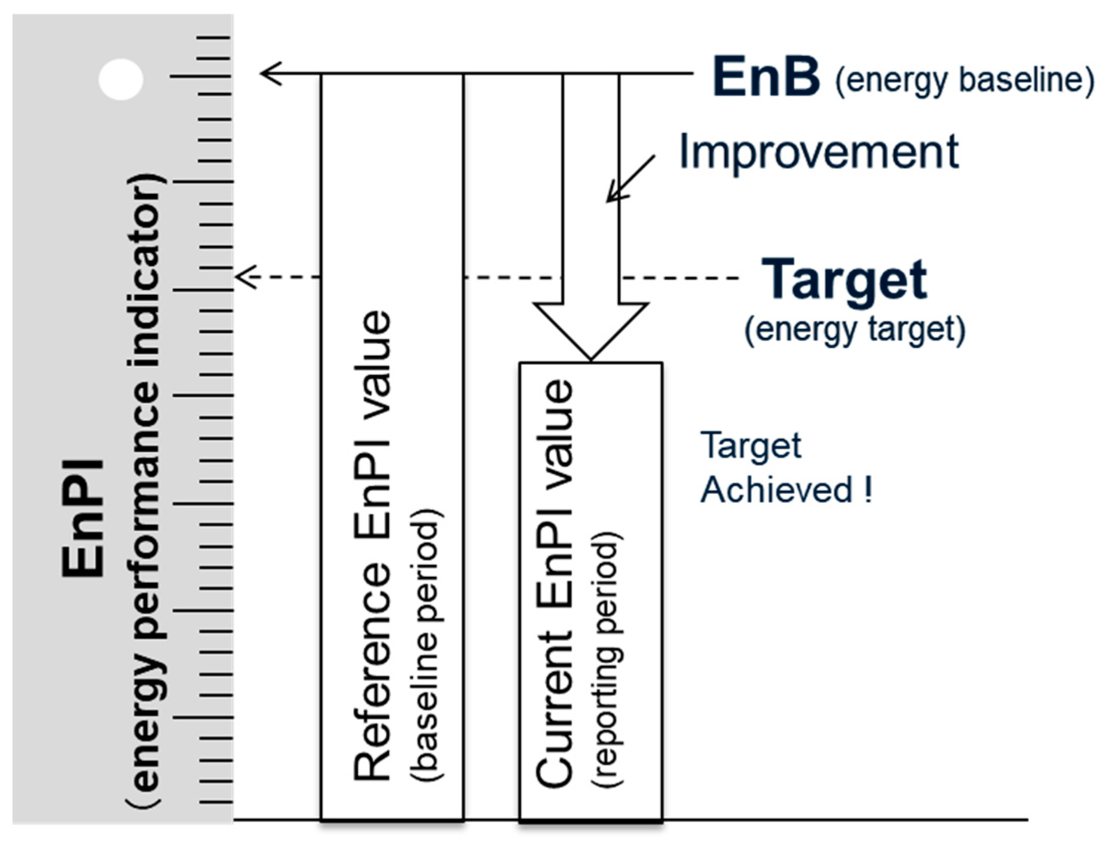
Conversely, the endeavor to inaugurate a novel energy baseline (EnBL) entails the meticulous collection of precise and representative data concerning energy consumption within the pertinent system or process. These requisite data can be acquired through the deployment of instrumentation, real-time monitoring protocols, and systematic energy audits. It is imperative to underscore the intrinsic correlation between the energy baseline and Energy Performance Indicators (EnPIs). EnPIs serve as pivotal tools for gauging the energy performance of a given system or process, and they are juxtaposed against the established EnBL, as elucidated in Figure 1 [26].
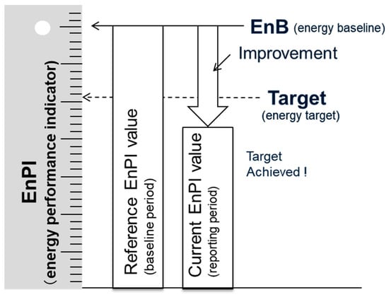
Figure 1.
Base period concept and reference period concept for IDE.
In the context of energy management systems, the primary function of an energy baseline is to provide a quantitative reference that serves as the foundation for comparing energy performance. The EnBL represents a value for electrical or thermal energy consumption that allows for the measurement of savings by establishing a reference point before and after the implementation of improvement actions. This baseline should account for factors such as the analysis period, established boundaries, the source and accuracy of data, and the relevant variables that impact energy consumption. Moreover, normalization processes should be incorporated to mitigate the effects of abnormal values in these relevant variables that influence energy consumption.
The energy baseline is essential for monitoring energy efficiency indicators, provided that it is supported by statistical validation, and for enabling reliable forecasts of future consumption levels.
To select an EnBL and EnPI [26], different models are available, as shown in Table 1. Table 1 shows EnB’’s strengths and weaknesses according to the type of method chosen.

Table 1.
Types of energy baselines (EnBLs).
2. Methodology
The designation of an energy baseline (EnBL) is contingent upon various factors such as the magnitude of the facility, occupancy rates within a structure, and prevailing climatic conditions, among other pertinent considerations. Moreover, this process necessitates a comprehensive comprehension of the objectives at hand, meticulous data acquisition and analysis, and rigorous validation to ascertain the utility of the chosen EnBL. This intricate procedure is instrumental in establishing a precise EnBL conducive to the accurate measurement of energy performance, thereby serving as a crucial mechanism for assessing the efficacy of energy efficiency initiatives.
Figure 2 delineates a methodological schematic elucidating the sequential steps inherent in the selection of a model for the establishment of both EnBL and Energy Performance Indicators (EnPI). The evaluation of energy performance enhancement within a building entails the quantification of energy consumption, the normalization of variables germane to its consumption, the utilization of models for EnBL and indicators substantiated by requisite statistical validations, and the computation of improvements in energy performance. This multifaceted process culminates in the quantification of energy saving and efficiency levels.
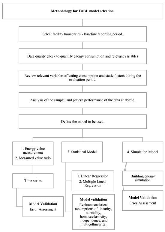
Figure 2.
Methodology for LBE model selection.
2.1. Energy Value Model and Measured Value Ratio
In the pursuit of enacting an energy baseline (EnBL) through the utilization of the absolute consumption model and specific energy consumption, a recommended methodology involves the employment of statistical analyses founded on time series. A time series, in this context, denotes an assemblage of numerous observations pertaining to a variable measured at consecutive temporal intervals or successive time periods [27].
The primary objective of a time series resides in the discernment of discernible patterns within historical data, subsequently extrapolating these patterns into prospective temporal domains. This prognostication is predicated solely upon past values of the variable or preceding forecast errors. The intricate composition of a time series data point’s pattern or performance emanates from diverse components, typically encompassing trend, cyclical, seasonal, and irregular elements.
Within the framework of a time series, several forecast models are available, depending on the historical data available, including the average historical monthly consumption, weighted average of historical monthly consumption, seasonality indexes, and order moving average, considering the average daily consumption trend.
A pivotal aspect of this process is the establishment of error measures, serving as evaluative tools to scrutinize the soundness of the executed forecasting model. These error measures facilitate the precision assessment of these forecasting methods, guiding the selection of the most optimal one [28,29]. The error associated with any forecast is the disparity between the observed value in the time series and the forecast itself. This forecast error may manifest as positive or negative, which is contingent upon whether the forecast overestimates or underestimates the actual value. The computation of forecast errors [30] typically follows Equation (1).
This formula facilitates informed decisions regarding the optimal forecasting method. It empowers the identification of anomalies or discrepancies in our demand forecast, enabling timely adjustments and redirection toward more judicious choices.
The Mean Absolute Percentage Error (MAPE) serves as a metric quantifying the deviation in percentage terms. It represents the mean absolute error, elucidating the variance between the actual demand and the forecasted values. This metric, also recognized as Percentage Error Mean Absolute (PEMA) (Equation (2)), stands as a robust tool for evaluating the precision of forecasting methodologies.
2.2. Statistical Models
Statistical regression methodologies have recurrently served as instrumental tools for the extrapolation of trend data and the prognostication of forthcoming performance. In the realm of estimating energy baseline (EnBL) and prognosticating energy consumption within architectural domains, the preponderance lies in the deployment of linear regression models. Eminent scholars, including Syarifah Permai and Heruna Tanty [31], Jonathan Roth and Ram Rajagopal [32], Nelson Fumo and Rafe Biswas [33], Beñat Arregi and Roberto Garay [34], and Aranda et al. [35], among others [36,37,38,39,40], have significantly advanced this line of inquiry. Nevertheless, a cohort of researchers, as exemplified by Bilous et al. [41], diverge in their approach, opting for the utilization of nonlinear regression models.
Numerous investigations have been conducted to approximate the energy baseline (EnBL), employing both univariate and multivariate regression models. Rigorous examinations of these models have been undertaken to ensure compliance with a battery of statistical assumptions requisite for the validation of the regression framework. Strachan [42] adeptly utilized this methodology to prognosticate energy consumption levels within the United Kingdom, leveraging it as a strategic instrument in the formulation of energy policies. Sakamoto et al. [43], in a parallel vein, harnessed the baseline model to foresee Japan’s energy requisites for the year 2030, meticulously incorporating climatic variables and socio-economic facets of the nation. The outcome of their investigation illuminated an upward trajectory in the building sector’s energy consumption juxtaposed with a concomitant downturn in industrial usage.
Alves et al. [44], Ko et al. [45], and Elbeltagi et al. [46] assert that the construction of an EnBL serves as a pivotal precursor to comprehending the energy demands of urban landscapes bereft of benchmarks for building energy consumption. This lacuna in knowledge complicates decision-making concerning building stock management, given the absence of knowledge pertaining to both extant and achievable energy performance. Liang et al. [47], in a noteworthy observation, contend that extant models for predicting EnBLs in buildings frequently neglect occupancy as a variable, which is an oversight considered to be pivotal in antecedent research [48].
Regression methodologies, as applied in this context, scrutinize the formulation of models elucidating the interdependence between a dependent variable (Y) and explanatory variables (X). These models typically adopt either univariate or multivariate configurations. The univariate instantiation is explicated by Equation (4).
The multivariable model is defined by Equation (4).
Typically, the assessment of regression models hinges upon the proportion of variance in the dependent variable that can be explained by the independent variables. This elucidation is encapsulated by the coefficient of determination, denoted as R2, which is a metric ranging from 0% to 100%. Consequently, an elevated R2 value signifies the heightened accuracy of the model in accordance with the available data.
Nevertheless, the mere attainment of a lofty R2 value within a regression model does not unequivocally ensure optimal predictive efficacy. It is imperative, therefore, to adhere to a suite of statistical assumptions to substantiate the validity of the model. The necessary statistical assumptions that regression models are required to satisfy Linearity, Normality, Homoscedasticity, Independence, and Multicollinearity (Only for the multivariable model) [49,50,51,52]. Table 2 shows the statistical assumptions that regression models must fulfill.

Table 2.
Statistical assumptions for the regression model.
2.3. Simulation Models
Simulation serves as a pivotal avenue for experimental exploration within a model, affording insights into system performance and the judicious evaluation of novel strategies within the confines demarcated by predefined criteria [53,54].
The raison d’être of energy simulation lies in the meticulous modeling of a building and its ambient milieu, thereby prognosticating its forthcoming energy performance [55]. This necessitates the comprehensive consideration of intrinsic architectural attributes (such as geometry and materials), meteorological conditions, and operational parameters (inclusive of occupancy levels, operational hours, internal loads, etc.).
The simulation of energy dynamics within the architectural realm facilitates a temporal analysis of a building’s energy requisites, concurrently ensuring the provision of fundamental comfort conditions congruent with its design and environmental context [53]. It emerges as a highly efficacious instrument for attaining equilibrium between energy consumption, economic considerations, comfort provisioning, and environmental sustainability.
In contemporary discourse, energy simulation within the built environment assumes an indomitable role in advancing the frontiers of energy consumption optimization and efficiency. This is achieved through the utilization of computational tools, which enable the comprehensive evaluation of the energy performance of buildings and their installations [56,57]. By leveraging authentic data acquired through direct measurements, energy simulation validates the existing state of a structure, subsequently engendering recommendations for enhancements and the amelioration of energy consumption.
Dynamic simulations of buildings are facilitated by sophisticated software (V7) applications designed explicitly for the assessment of energy consumption. Foremost among these and enjoying widespread international acclaim are EnergyPlus, Design Builder, TRNSYS, and Equest.
3. Case Study
A classroom building on the UAO University campus (Figure 3), is studied as an application of the EnBL. The UAO University campus has seven buildings in operation [58]. The campus has four classroom buildings with four floors, offices, and classrooms mainly for undergraduate and postgraduate classes, a university wellness building where offices and cafeterias are located, a gym building with lightning toward the football fields, and lots.

Figure 3.
Lecture hall building of a university campus.
On the UAO campus, electrical energy is distributed through 3 substations that feed different sectors of the campus. Substation one, with a capacity of 500 kVA, provides loads to the main building; substation two has a power capacity of 1000 kVA, and it feeds loads to the common areas of the campus, the four classroom buildings, the university wellness building, and the Physical Conditioning and Health Centre (CAFS). Substation three, with a capacity of 800 kVA, feeds the air conditioning system of the main building, except for its handlers. Regarding photovoltaic solar energy, there are eight solar systems on the roofs of parking lots, classrooms, the main building, and the university wellness building. The solar generation is connected to the nearest distribution boards; the total installed capacity is 404 kWp.
The UAO campus has an electrical energy measurement system that monitors consumption. This system has 19 SCHNEIDER meters with telemetry systems that collect information on active, reactive, and apparent power and energy with a 15-min periodicity; the data are reported and stored in Power Monitor-CGE software (V7).
The methodology proposed above is also used for study to analyze the best model for the selection of the EnBL.
Figure 4a,b show the southwest and northwest views of the lecture hall building, as designed using Design Builder software for dynamic energy simulation.

Figure 4.
Views of the building, modeled with Design Builder. (a) Southwest view. (b) Northeast view.
The boundaries of this research are set on the case study. The analysis period corresponds to three consecutive years.
Experimental data have been obtained through monitoring. The data used for the analysis of the different methods applied to obtain LBEn are energy monitoring data with a recording frequency of 15 min per variable, data from the weather station installed at the university and the IDEAN weather station, and occupancy data. In this case, the data include the semester schedule of classes and the occupancy.
Several issues related to data precision have been identified, particularly the lack of calibration in several installed meters and the recurrent communication failures between the meters and data management software, which result in unrecorded measurements. These are systematic errors that significantly affect data analysis and the accuracy of forecasting models. Additionally, in terms of building occupancy, there is uncertainty related to academic scheduling and the use of classrooms, auditoriums, and offices, further complicating energy consumption predictions.
The analyses of the relevant variables and static factors include the information provided during the study period. As a whole, they include data from meteorological stations installed at the UAO University that provide the climatological variables. In addition, information on educational planning is obtained that is related to the occupation of different spaces and the energy consumption of the building. The final energy consumption of the building is also obtained. In this case, it constitutes the dependent variable. It comprises the consumption of the electric meter located in the building, plus the energy generated by the photovoltaic (PV) panels installed on the roof.
The daily dry outdoor air temperature is calculated from the hourly information available from the weather station. The daily relative humidity of the outside air is available from the weather station.
The average solar radiation is calculated considering the daily radiation time (direct and diffuse radiation). In addition, the occupancy of people in the classroom building corresponding to students is expressed in units of time of use per room. The consumptions can be seen in the trend graphs of the building, which are fixed consumptions that are measured even without occupancy in the building.
Data analysis and performance are among the most important initial elements in the decision to use a particular EnBL model. According to the provenance, verification, and frequency of the data, together with possible alterations in terms of the registration, it will be decided which type of EnBL model to use for the data.
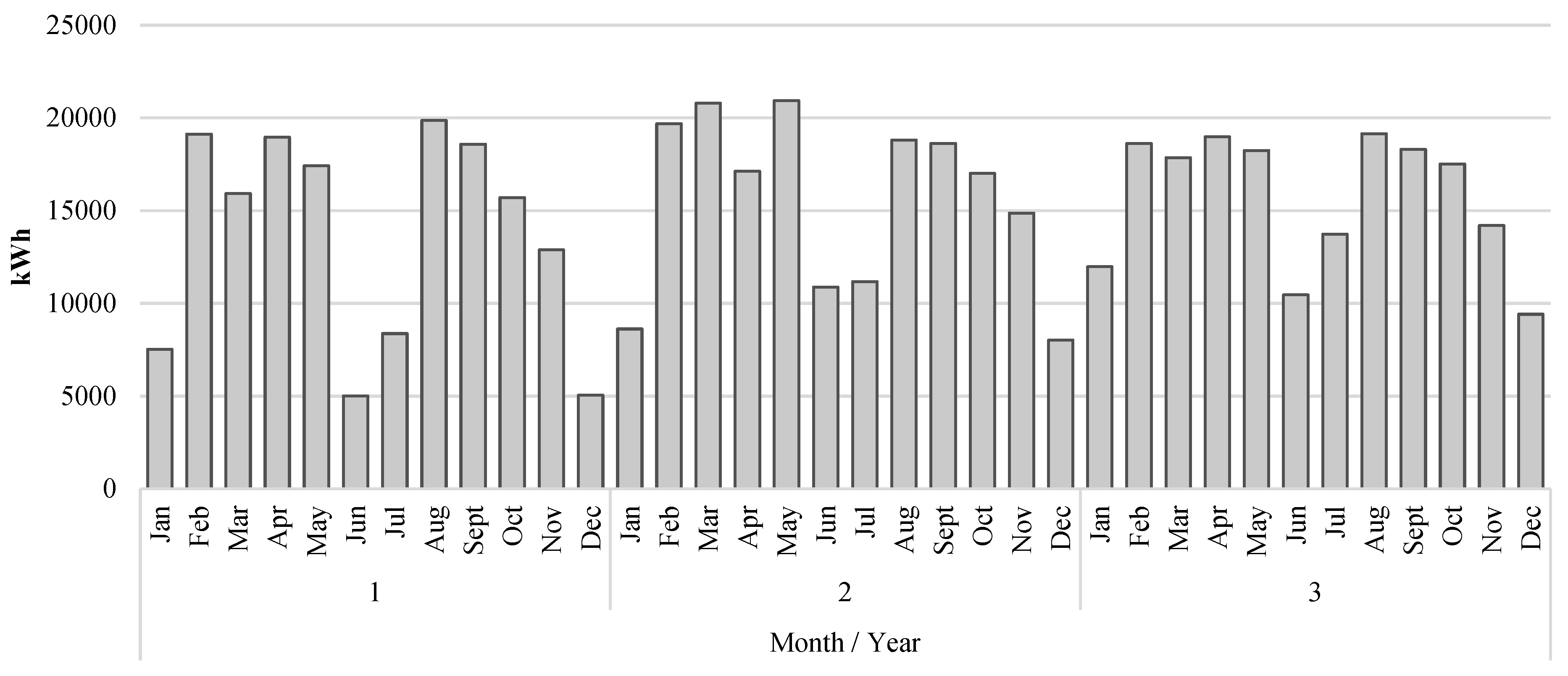
Figure 5 shows monthly measurements of the final energy consumption of the UAO University’s Aulario building for three consecutive years.
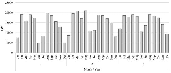
Figure 5.
Monthly electricity consumption of the lecture hall building of the UAO University campus.
The analysis of historical monthly electricity consumption data for Classroom 4 (Figure 5) reveals a clear annual seasonal pattern, with a slight disruption noted between March and April that is contingent upon the timing of Holy Week, during which the university is closed. Additionally, there is a significant annual increase in energy consumption (Figure 6), which can be attributed to the progressive technological upgrades implemented in Classroom 4. Specifically, in the year analyzed, this increase amounted to 13.5% compared to the previous year, while the subsequent year exhibited a more modest rise of only 1.0%.
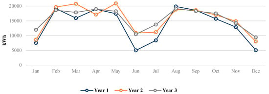
Figure 6.
Seasonal performance of final energy consumption of the lecture hall building.
The analysis of electricity consumption monitoring in the lecture hall building (Figure 6) shows an annual seasonal performance with a small discrepancy between March and April that depends on the month in which Easter week is celebrated as a holiday week as the building is closed during this time.
4. Analysis and Results
Once the information from energy monitoring has been obtained, the use of time series models applied to obtain an energy baseline, LBEn, is shown. This is considered a proposal for the validation of the energy value measurement models and for the quotient of measured values. The fundamental purpose of LBEn is to provide a quantitative reference that serves as a basis for the comparison of energy performance, allowing the measurement of savings as a reference for the implementation of improvement strategies. Considering this as a reference value of consumption of any type of energy, the time series analysis fits well with the previously mentioned models.
4.1. EnBL Time Series Models
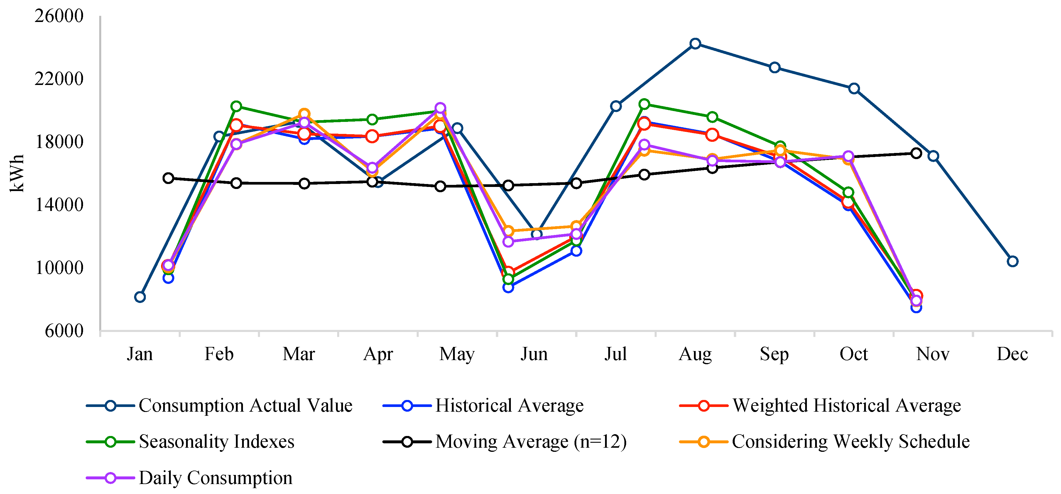
The time series models proposed for validating energy value measurement models and the ratio of measured values are applied to establish an energy baseline. This application is illustrated through the case study of Classroom 4 on the university campus, progressing from simple models to those that account for seasonality and segmented data analysis. Over a three-year period, an analysis was conducted using each proposed time series model, revealing variations in the Mean Absolute Percentage Error (MAPE) ranging from 1.1% among the Historical Average, Weighted Historical Average, and Seasonality Indices models. Conversely, the Moving Average model (n = 12) exhibited the highest error rate, underestimating consumption values during low-demand months. The models considering the weekly schedule and daily consumption demonstrated improved accuracy by incorporating relevant variables such as the academic scheduling of classrooms and average daily consumption.
The six time series models obtained for forecasting the energy consumption of the building are summarized below. Table 3 and Figure 7 show the values obtained for the different models compared with the actual energy consumption.

Table 3.
Six forecasting models implemented to determine the energy consumption in kWh and the actual value of energy consumption.
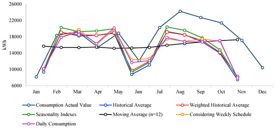
Figure 7.
Results of the different forecasting methods to obtain an annual LBEn for the building.
To compare the six different time series forecasting models used in order to obtain the LBEn, the Mean Absolute Percentage Error (MAPE) was used. MAPE provides the deviation in percentage terms and is presented in Table 4.

Table 4.
Mean Absolute Percentage Error (MAPE) for time series models.
4.2. Univariate and Multivariate Linear Regression Models for EnBL
To build a reliable linear regression model, the independent variables that may have a high correlation with the variable to be explained are first identified. Using RStudio software (V7), the correlation levels of the independent variables (temperature, humidity, radiation, and total occupancy) presented in Table 5 were obtained regarding the dependent variable (total final energy consumption).

Table 5.
Mean values of variables monitored in the building.
To ensure that the statistical forecasting model performed is valid [9], a series of statistical tests were carried out considering: The regression function is nonlinear; The error terms are not normally distributed; The error terms have non-constant variance; The error terms are not independent; The independent variables are not related to each other (for the multivariate case).
Table 6 shows details of compliance with the different statistical assumptions, according to their test and graphical representation.

Table 6.
Assumptions and verification tests for regression models.
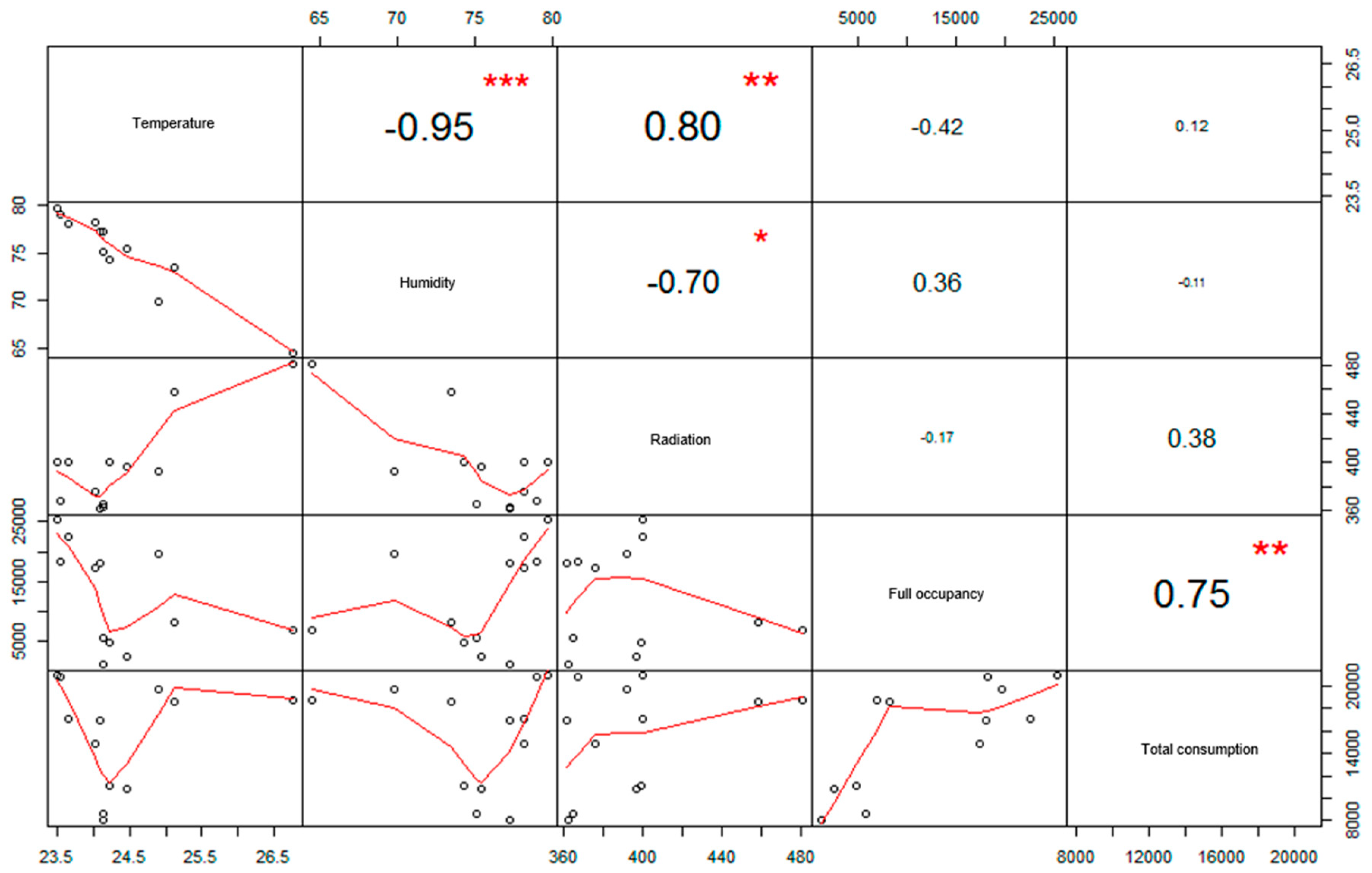
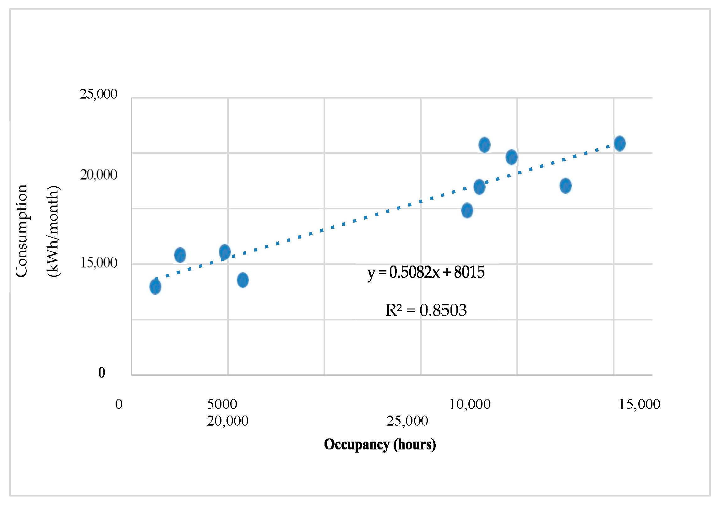
Four univariate linear regression models were calculated with different variables (temperature, humidity, radiation, and total occupancy). In order to validate the results, Figure 8 graphically shows the relation between the variables and their statistical significance from highest to lowest (red asterisks, *** > ** > *). The variable with the highest correlation and statistical significance, which allows for the description of the Total Energy Consumption variable, is the independent variable Total Occupancy. However, this model has a somewhat low coefficient of determination. For this reason, the residuals method was applied in order to filter out some outliers and improve the coefficient of determination R2, allowing an increase in the correlation level to R2 = 0.8503.
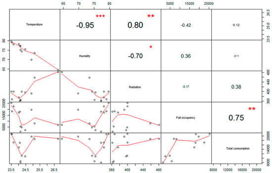
Figure 8.
Total final energy consumption correlation with independent variables—RStudio software.
The model was able to explain 85.03% of the data variability. Similarly, the p value of 0.0001 was analyzed for the F-statistic, which indicates that the linear correlation is statistically significant (0.0001 < 0.05).
The confidence intervals of the model have significance levels of 2.5–97.5%, which is the range in which the univariate linear regression model can vary. The results of the global test (gvlma) confirm that all assumptions of the univariate linear regression model are verified. It is valid to use the linear regression model to quantify energy consumption as a function of the relevant independent variable (“Total occupancy”).
The univariate linear regression model carried out (Figure 9) is described by Equation (5):
EnBL Consumption = 0.5082 ∙ Occupancy + 8015 + εi

Figure 9.
EnBL of classroom energy consumption (kWh/month) vs. total occupancy (hours).
In this study, a multivariate linear regression model was also conducted for one year, with all the available variables (temperature, humidity, radiation, and total occupancy). The statistical analysis of the variables for one year shows that the variables temperature and radiation are not significant in the multivariate linear regression model, since their p values are greater than 0.05. In this case, the significant variables in the model are the outdoor humidity and the occupancy variable.
The optimal multivariate linear regression model built in RStudio statistical software is (Equation (6)):
The model has an adjusted R2 = 0.9082, indicating that the model explains 90.82% of the variability in the observations (data).
The adjusted R2 value measures the percentage of the variance in the model’s response; however, it adjusts for the number of predictor variables in the model. The model has a p value of 8.7 × 10⁻⁶ for the F-statistic, indicating that the linear correlation is statistically significant (8.7 × 10⁻⁶ < 0.05). To ensure that the model is valid, the overall test of statistical assumptions and the multicollinearity test were performed.
Global test results (gvlma) and VIF test results for multicollinearity confirm that the regression model performed complies with the statistical assumptions. This result means it is valid for quantifying energy consumption as a function of the relevant variables “humidity” and “total occupancy”. Table 7 shows a comparison of the estimated energy consumption of EnBL with the monitored energy consumption of the building and the MAPE forecast error.

Table 7.
Comparison of estimated energy consumption of EnBL with the monitored energy consumption of the building and the MAPE.
4.3. EnBL Simulation Model
Simulation is another methodology to obtain EnBL. This technique consists of designing a model for a real system and experimenting with it in order to understand the energy performance of the building.
The energy simulation of the building is carried out using an internationally recognized software, Design Builder, with the EnergyPlus calculation engine.
This simulation model has been calibrated with experimental data measured by monitoring through a Building Management System (BMS) system.
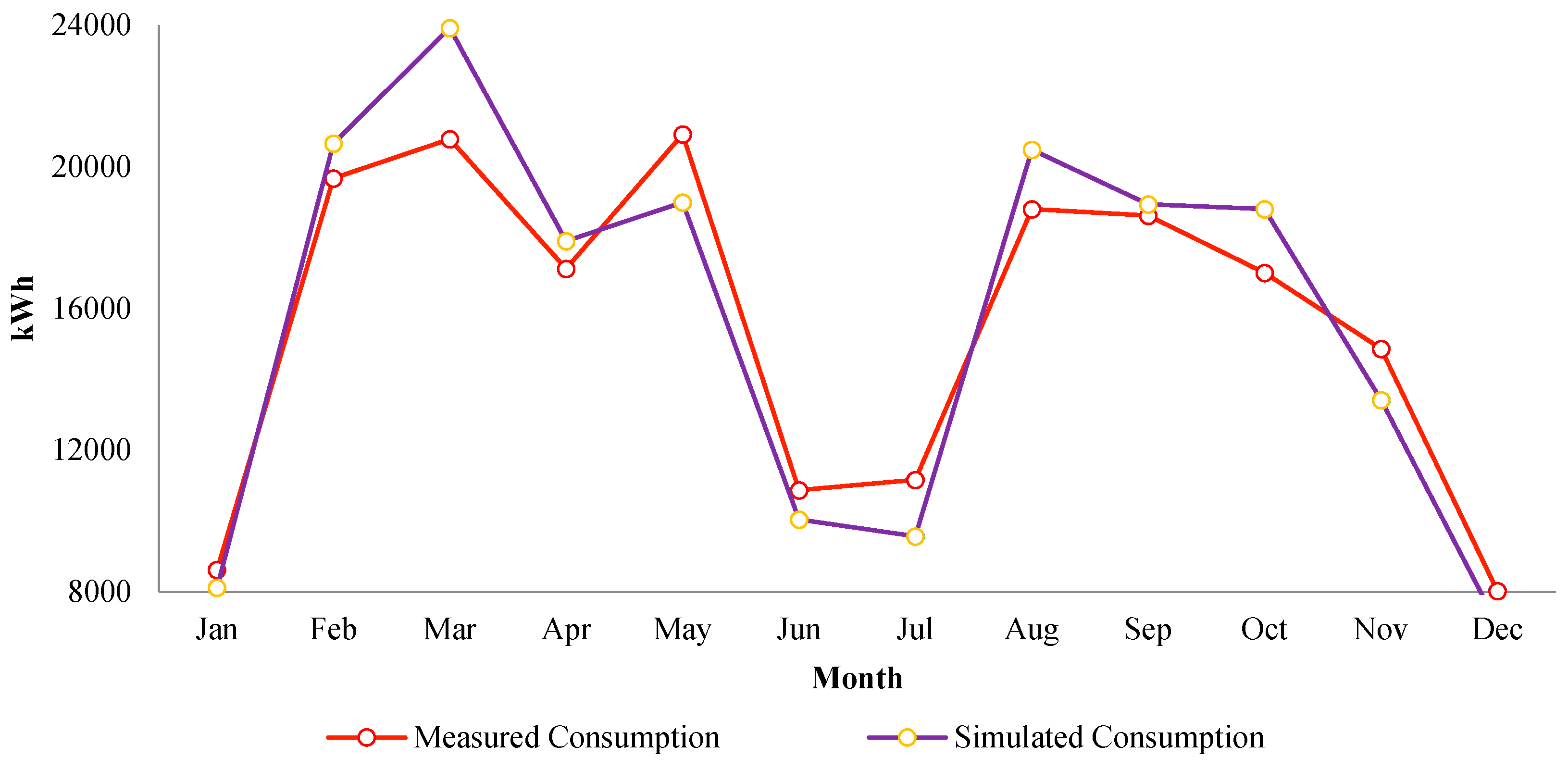
Figure 10 shows the difference between energy consumption (typical year) and measured data by monitoring, where it can be seen that the months with the lowest energy consumption correspond to January, June, and December; these months are vacation days in the university calendar.
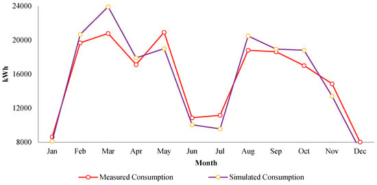
Figure 10.
Simulated vs. monitored energy consumption.
At the same time, the error between the simulated and experimentally measured energy consumption is reduced, adjusting the simulated model to an annual error of less than 1%. There are 4 months that slightly exceed 10%.
The energy demand is satisfied by the final electrical energy; it is partly generated with the renewable PV system available in the building, and another part is supplied by the grid.
Table 8 shows the data obtained by calibrating the EnergyPlus simulated model of the building.

Table 8.
Monitored and simulated power consumption values.
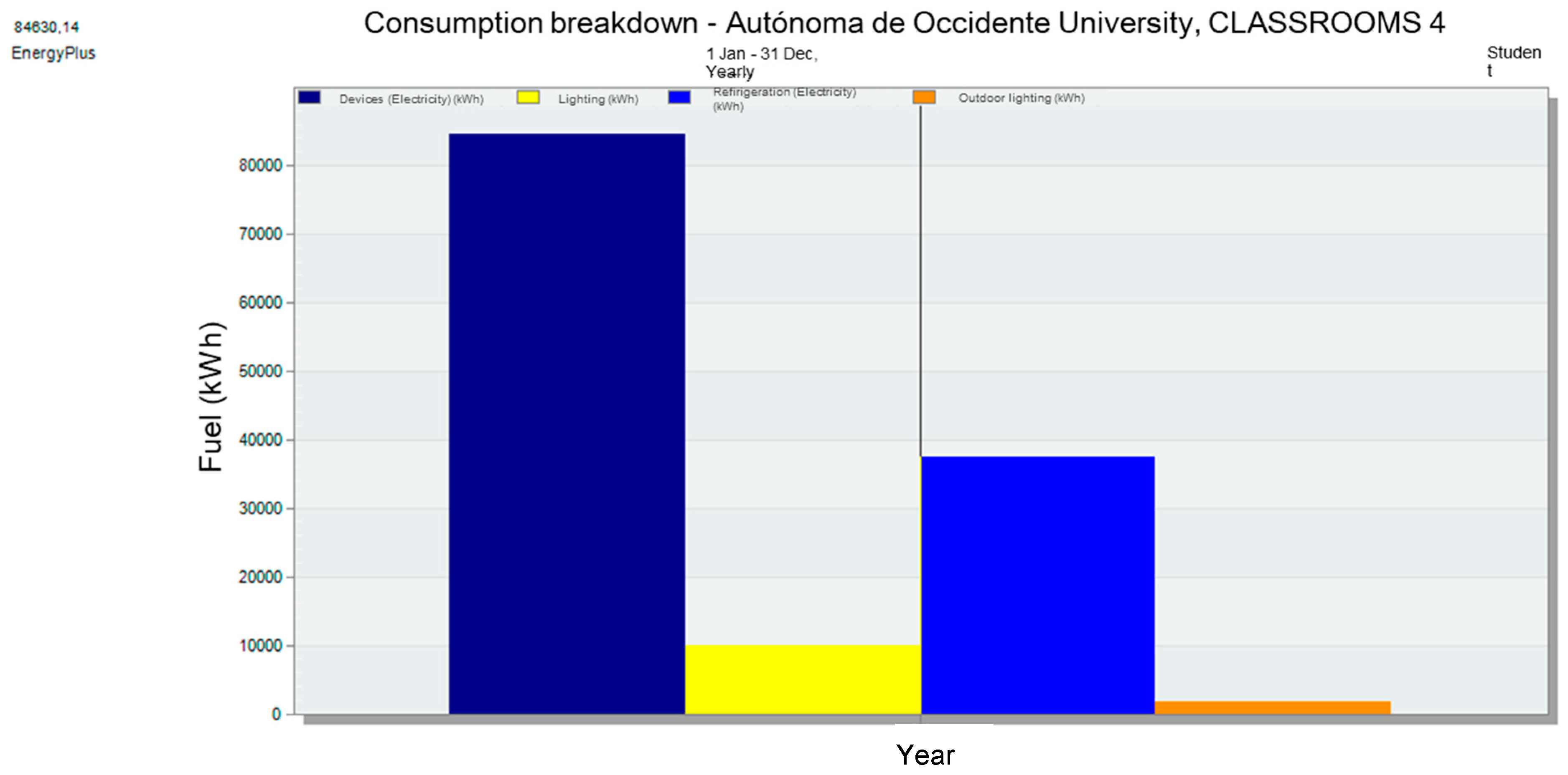
Figure 11 shows the energy consumption broken down by items for the building.
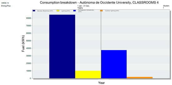
Figure 11.
Electrical consumption breakdown of the building. Devices: 84,630.14 kWh, Lighting 10,014.03 kWh, Refrigeration: 37,466.96 kWh, Outdoor lighting: 1735.83 kWh.
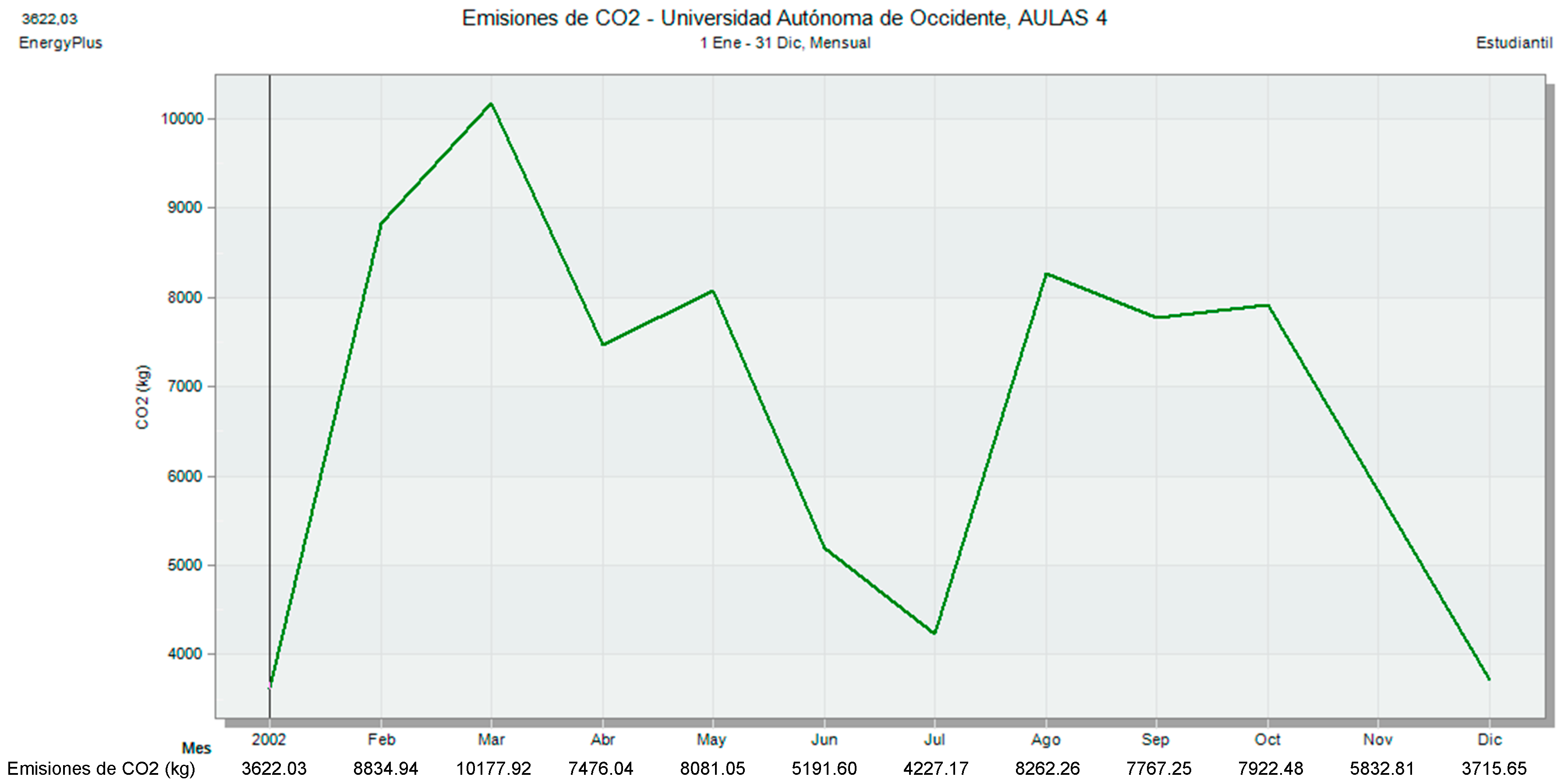
Figure 2 shows the emissions generated in the building on a monthly basis and an annual basis (Figure 12). Thus, in addition to achieving the LBEn, it informs us of the building’s operational carbon footprint and how to improve it.
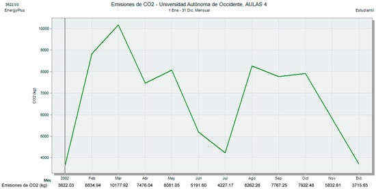
Figure 12.
CO2 emissions for the lecture hall building.
The simulation model not only assists in the validation and selection of energy baselines for buildings but also provides a framework for ensuring the validity of forecast results and the use of appropriate indicators, ultimately filling regulatory gaps in terms of mathematical and statistical models required for norm compliance.
5. Discussion
The quality of data and the varying levels of measurement present one of the most significant limitations in applying the proposed methodology for establishing an energy baseline in buildings. This limitation is closely tied to the degree of monitoring in buildings across different contexts and sectors. However, the methodology provides opportunities to estimate the baseline using available data resources, allowing for more accurate saving projections based on the level of monitoring and the inclusion of variables that may affect energy consumption.
The choice of model depends on the availability of data, particularly the frequency and number of variables associated with consumption. For buildings that only have access to monthly billing data, a time series model is appropriate. In contrast, if real-time consumption data, weather variables, and occupancy-related factors are available, linear and multivariable regression models provide more accurate baseline estimates for forecasting energy consumption. This analysis aims to present a range of possibilities by validating mathematical and statistical tools when selecting a model to establish an energy baseline. The developed models demonstrate that the choice of model influences the overestimation or underestimation of energy consumption forecasts, which in turn impacts saving calculations. Time series models are functional when only energy consumption data is available, serving as a starting point for building management. On the other hand, regression models yield more precise results for building operations by accounting for climate conditions, occupancy levels, equipment usage, and other factors.
Statistical tests are essential to determine which model best describes and reflects the energy consumption trends in the facility. These tests also help assess whether the energy performance improvement percentages make sense in relation to the facility’s operational patterns and the selected baseline reporting periods.
The use of different models can lead to either underestimation or overestimation of energy savings, and statistical validation plays a critical role in selecting the model with the best predictive accuracy and lowest error. In this regard, the ability to use different models tailored to the needs and data resources of the building allows for the identification of initial savings, which can be adjusted as monitoring systems evolve and relevant variables and static factors affecting consumption are identified. The methodology enables the selection of a model according to the level of monitoring, which is crucial for the accuracy of saving estimates and their subsequent realization. The limitations observed in the four models proposed for baseline estimation are primarily associated with data quality, specifically data frequency and measurement gaps. These issues are recurrent in energy monitoring systems, often stemming from communication problems between meters and the management software. Challenges arise in defining the boundaries and ranges used to establish the baseline, which must account for building occupancy, seasonality, and the need to segment analysis periods based on the building’s operational activities.
Another key element is identifying the relevant variables that influence energy consumption. Statistical tests (e.g., p value criteria) can help determine whether these variables significantly impact energy consumption and should therefore be used for normalization. Statistical verification of error percentages and compliance with statistical assumptions is essential to ensure that the baseline is valid for setting energy saving targets and implementing reliable energy efficiency indicators.
6. Conclusions
This study provides a comprehensive analysis of methodologies for estimating the energy baseline (EnBL) in university classroom buildings, aimed at improving energy efficiency and supporting decarbonization efforts. Four methodologies are proposed: time series models, univariate regression models, multivariate regression models, and dynamic simulations using Design Builder software.
To identify the most suitable model, we established criteria for selecting limits, analysis periods, data quality, and relevant variables that were validated through statistical analysis of daily monitoring data using RStudio software. Dynamic simulations demonstrate significant advantages by allowing the exploration of various operational scenarios, including interactions among lighting, HVAC systems, and office equipment. This enhances the accuracy of energy consumption predictions and establishes reliable baselines for both new and existing buildings.
Each model underwent rigorous statistical validation and error analysis, addressing regulatory gaps related to the application of mathematical models and ensuring compliance with standards lacking clear foundations for baseline validation. The choice of the EnBL estimation model significantly impacts projected energy savings: time series models effectively analyze energy consumption data alone, while regression models enhance accuracy by including climate and occupancy factors. Dynamic simulation emerges as the most precise method when calibrated correctly with the EnergyPlus engine.
By simulating diverse building usage scenarios, we gained a comprehensive understanding of energy consumption patterns, aiding in the development of effective optimization strategies. The robust validation of the energy baseline through statistical analysis increases confidence in energy saving predictions, which is essential for informed decision-making.
The monthly models illustrate the proposed energy management methodology, with associated errors of 8.2%, 1.2%, 2.2%, and 0.5% for the daily, weekly, monthly, and proposed baselines, respectively. While the daily baseline model performs well during normal operational months, it struggles in July when occupancy drops significantly. In contrast, the weekly and monthly models provide improved forecasting results through better variable integration.
This study offers a structured framework for selecting the appropriate EnBL estimation methodologies, emphasizing the importance of statistical validation for accurate results. The use of simulation models enhances transparency and reliability in energy performance assessments, positioning them as essential tools for improving energy efficiency and meeting regulatory standards in building design and operation. The insights gained are crucial for optimizing energy consumption in building sustainability.
Author Contributions
Conceptualization, R.C.-M. and F.J.R.-M.; methodology, R.C.-M. and J.M.R.-H.; software, R.C.-M. and L.C.-M.; validation, L.C.-M. and F.J.R.-M.; formal analysis, J.M.R.-H., L.C.-M. and F.J.R.-M.; investigation, R.C.-M., J.M.R.-H., L.C.-M. and F.J.R.-M.; data curation, R.C.-M., L.C.-M. and J.M.R.-H.; writing—original draft preparation, R.C.-M., F.J.R.-M. and J.M.R.-H.; writing—review and editing, R.C.-M. and J.M.R.-H.; visualization, F.J.R.-M.; supervision, F.J.R.-M. All authors have read and agreed to the published version of the manuscript.
Funding
This research received no external funding.
Data Availability Statement
The original contributions presented in the study are included in the article, further inquiries can be directed to the first author.
Acknowledgments
This paper has been made possible due to the support received from “LIFE23-CET-Re-Energize” Project by University of Málaga, Spain, “Lime4Health” Project by Technical University of Madrid (UPM), RED-TRAPECIO Project by CYTED, Vice Rector’s Office for Research, Innovation and Entrepreneurship at UAO University, and ITAP Research Institute at University of Valladolid.
Conflicts of Interest
The authors declare no conflicts of interest.
References
- ISO. ISO 50001:2018 Energy Management Systems—Requirements with Guidance for Use; ISO: Geneva, Switzerland, 2018. [Google Scholar]
- Fuchs, H.; Therkelsen, P.; Miller, W.C.; Siciliano, G.; Sheaffer, P. ISO 50001-Based Energy Management Systems as a Practical Path for Decarbonization: Initial Findings from a Survey of Technical Assistance Cohort Participants. Energies 2023, 16, 5441. [Google Scholar] [CrossRef]
- Fuchs, H.; Aghajanzadeh, A.; Therkelsen, P. Identification of Drivers, Benefits, and Challenges of ISO 50001 through Case Study Content Analysis. Energy Policy 2020, 142, 111443. [Google Scholar] [CrossRef]
- McKane, A.; Therkelsen, P.; Scodel, A.; Rao, P.; Aghajanzadeh, A.; Hirzel, S.; Zhang, R.; Prem, R.; Fossa, A.; Lazarevska, A.M.; et al. Predicting the Quantifiable Impacts of ISO 50001 on Climate Change Mitigation. Energy Policy 2017, 107, 278–288. [Google Scholar] [CrossRef]
- Fitzgerald, P.; Therkelsen, P.; Sheaffer, P.; Rao, P. Deeper and Persistent Energy Savings and Carbon Dioxide Reductions Achieved through ISO 50001 in the Manufacturing Sector. Sustain. Energy Technol. Assess. 2023, 57, 103280. [Google Scholar] [CrossRef]
- Andersson, E.; Dernegård, H.; Wallén, M.; Thollander, P. Decarbonization of Industry: Implementation of Energy Performance Indicators for Successful Energy Management Practices in Kraft Pulp Mills. Energy Rep. 2021, 7, 1808–1817. [Google Scholar] [CrossRef]
- U.S. Department of Energy. 50001 Ready Cohorts: Technical Assistance to Implement Energy Management Systems; U.S. Department of Energy: Washington, DC, USA, 2023. [Google Scholar]
- Chan, D.Y.L.; Huang, C.F.; Lin, W.C.; Hong, G.B. Energy Efficiency Benchmarking of Energy-Intensive Industries in Taiwan. Energy Convers. Manag. 2014, 77, 216–220. [Google Scholar] [CrossRef]
- El Majaty, S.; Touzani, A.; Kasseh, Y. Results and Perspectives of the Application of an Energy Management System Based on ISO 50001 in Administrative Buildings—Case of Morocco. Mater. Today Proc. 2023, 72, 3233–3237. [Google Scholar] [CrossRef]
- Jovanović, B.; Filipović, J.; Bakić, V. Energy Management System Implementation in Serbian Manufacturing—Plan-Do-Check-Act Cycle Approach. J. Clean. Prod. 2017, 162, 1144–1156. [Google Scholar] [CrossRef]
- Thollander, P.; Karlsson, M.; Söderström, M.; Creutz, D. Reducing Industrial Energy Costs through Energy-Efficiency Measures in a Liberalized European Electricity Market: Case Study of a Swedish Iron Foundry. Appl. Energy 2005, 81, 115–126. [Google Scholar] [CrossRef]
- Fichera, A.; Volpe, R.; Cutore, E. Energy Performance Measurement, Monitoring and Control for Buildings of Public Organizations: Standardized Practises Compliant with the ISO 50001 and ISO 50006. Dev. Built Environ. 2020, 4, 100024. [Google Scholar] [CrossRef]
- Prashar, A. Energy Efficiency Maturity (EEM) Assessment Framework for Energy-Intensive SMEs: Proposal and Evaluation. J. Clean. Prod. 2017, 166, 1187–1201. [Google Scholar] [CrossRef]
- de Sousa Jabbour, A.B.L.; Verdério Júnior, S.A.; Jabbour, C.J.C.; Leal Filho, W.; Campos, L.S.; De Castro, R. Toward Greener Supply Chains: Is There a Role for the New ISO 50001 Approach to Energy and Carbon Management? Energy Effic. 2017, 10, 777–785. [Google Scholar] [CrossRef]
- Ocampo Batlle, E.A.; Escobar Palacio, J.C.; Silva Lora, E.E.; Martínez Reyes, A.M.; Melian Moreno, M.; Morejón, M.B. A Methodology to Estimate Baseline Energy Use and Quantify Savings in Electrical Energy Consumption in Higher Education Institution Buildings: Case Study, Federal University of Itajubá (UNIFEI). J. Clean. Prod. 2020, 244, 118551. [Google Scholar] [CrossRef]
- Awan, M.B.; Sun, Y.; Lin, W.; Ma, Z. A Framework to Formulate and Aggregate Performance Indicators to Quantify Building Energy Flexibility. Appl. Energy 2023, 349, 121590. [Google Scholar] [CrossRef]
- Usman, A.M.; Abdullah, M.K. An Assessment of Building Energy Consumption Characteristics Using Analytical Energy and Carbon Footprint Assessment Model. Green Low-Carbon Econ. 2023, 1, 28–40. [Google Scholar] [CrossRef]
- Yin, S.; Liu, L.; Mahmood, T. New Trends in Sustainable Development for Industry 5.0: Digital Green Innovation Economy. Green Low-Carbon Econ. 2023, 4, 1–13. [Google Scholar] [CrossRef]
- Palomar-Torres, A.; Rey-Hernández, J.M.; Rey-Hernández, A.; Rey-Martínez, F.J. A Novel Life Cycle Assessment Methodology for Transitioning from NZEB to ZEB. Case-Study. J. Build. Eng. 2024, 97, 110868. [Google Scholar] [CrossRef]
- Rey-Hernández, J.M.; Rey-Martínez, F.J.; Sala-Lizarraga, J.M.; Picallo-Perez, A. Innovative Exergy Indicators for Analyzing an NZEB Building to Promote New Areas of Improvement. Sustain. Energy Technol. Assess. 2024, 69, 103917. [Google Scholar] [CrossRef]
- Dmaidi, S.; Dwaikat, L.N.; Hussein, M.H. Energy Consumption Baseline for Public Schools in the West Bank-Palestine. Environ. Chall. 2024, 15, 100914. [Google Scholar] [CrossRef]
- Nnene, O.A.; Senshaw, D.; Zuidgeest, M.H.P.; Hamza, T.; Grafakos, S.; Oberholzer, B. Baseline Scenario Modelling for Low Emissions Development in Ethiopia’s Energy Sector. Energy Strateg. Rev. 2023, 49, 101166. [Google Scholar] [CrossRef]
- Afroz, Z.; Gunay, H.B.; O’Brien, W.; Newsham, G.; Wilton, I. An inquiry into the capabilities of baseline building energy modelling approaches to estimate energy savings. Energy Build 2021, 244, 111054. [Google Scholar] [CrossRef]
- Morvay, Z.K.; Gvozdenac, D.D. Applied Industrial Energy and Environmental Management; Wiley: Hoboken, NJ, USA, 2008; ISBN 9780470697429. [Google Scholar]
- Qaisar, I.; Zhao, Q. Energy baseline Prediction for Buildings: A Review. Results Control Optim. 2022, 7, 100129. [Google Scholar] [CrossRef]
- ISO. ISO 50006 Energy Management Systems—Measuring Energy Performance Using Energy baselines (EnB) and Energy Performance Indicators (EnPI)—General Principles and Guidance; ISO: Geneva, Switzerland, 2016. [Google Scholar]
- Anderson, D.R.; Sweeney, D.J.; Williams, T.A. Statistics for Business and Economics; South-Western: Nashville, TN, USA, 2011; ISBN 978-0538481649. [Google Scholar]
- Mouakher, A.; Inoubli, W.; Ounoughi, C.; Ko, A. EXPECT: EXplainable Prediction Model for Energy ConsumpTion. Mathematics 2022, 10, 248. [Google Scholar] [CrossRef]
- Mendoza-pittí, L.; Calderón-gómez, H.; Gómez-pulido, J.M.; Vargas-lombardo, M.; Castillo-sequera, J.L.; de Blas, C.S. Developing a Long Short-term Memory-based Model for Forecasting the Daily Energy Consumption of Heating, Ventilation, and Air Conditioning Systems in Buildings. Appl. Sci. 2021, 11, 6722. [Google Scholar] [CrossRef]
- Betancourt, D.F. Measuring Error in Demand Forecasts. Available online: https://ingenioempresa.com/medicion-error-pronostico/ (accessed on 10 November 2022).
- Permai, S.D.; Tanty, H. Linear Regression Model Using Bayesian Approach for Energy Performance of Residential Building. Procedia Comput. Sci. 2018, 135, 671–677. [Google Scholar] [CrossRef]
- Roth, J.; Rajagopal, R. Benchmarking Building Energy Efficiency Using Quantile Regression. Energy 2018, 152, 866–876. [Google Scholar] [CrossRef]
- Fumo, N.; Rafe Biswas, M.A. Regression Analysis for Prediction of Residential Energy Consumption. Renew. Sustain. Energy Rev. 2015, 47, 332–343. [Google Scholar] [CrossRef]
- Arregi, B.; Garay, R. Regression Analysis of the Energy Consumption of Tertiary Buildings. Energy Procedia 2017, 122, 9–14. [Google Scholar] [CrossRef]
- Aranda, A.; Ferreira, G.; Mainar-Toledo, M.D.; Scarpellini, S.; Llera Sastresa, E. Multiple Regression Models to Predict the Annual Energy Consumption in the Spanish Banking Sector. Energy Build. 2012, 49, 380–387. [Google Scholar] [CrossRef]
- Soebarto, V.I.; Williamson, T.J. Multi-Criteria Assessment of Building Performance: Theory and Implementation. Build. Environ. 2001, 36, 681–690. [Google Scholar] [CrossRef]
- Federspiel, C.; Zhang, Q.; Arens, E. Model-Based Benchmarking with Application to Laboratory Buildings. Energy Build. 2002, 34, 203–214. [Google Scholar] [CrossRef]
- Chung, W. Review of Building Energy-Use Performance Benchmarking Methodologies. Appl. Energy 2011, 88, 1470–1479. [Google Scholar] [CrossRef]
- Chung, W.; Hui, Y.V.; Lam, Y.M. Benchmarking the Energy Efficiency of Commercial Buildings. Appl. Energy 2006, 83, 1–14. [Google Scholar] [CrossRef]
- Filippín, C. Benchmarking the Energy Efficiency and Greenhouse Gases Emissions of School Buildings in Central Argentina. Build. Environ. 2000, 35, 407–414. [Google Scholar] [CrossRef]
- Bilous, I.; Deshko, V.; Sukhodub, I. Parametric Analysis of External and Internal Factors Influence on Building Energy Performance Using Non-Linear Multivariate Regression Models. J. Build. Eng. 2018, 20, 327–336. [Google Scholar] [CrossRef]
- Strachan, N. Business-as-Unusual: Existing Policies in Energy Model Baselines. Energy Econ. 2011, 33, 153–160. [Google Scholar] [CrossRef]
- Sakamoto, T.; Takase, K.; Matsuhashi, R.; Managi, S. Baseline of the Projection under a Structural Change in Energy Demand. Energy Policy 2016, 98, 274–289. [Google Scholar] [CrossRef]
- Alves, T.; Machado, L.; de Souza, R.G.; de Wilde, P. A Methodology for Estimating Office Building Energy Use Baselines by Means of Land Use Legislation and Reference Buildings. Energy Build. 2017, 143, 100–113. [Google Scholar] [CrossRef]
- Ko, J.H.; Kong, D.S.; Huh, J.H. Baseline Building Energy Modeling of Cluster Inverse Model by Using Daily Energy Consumption in Office Buildings. Energy Build. 2017, 140, 317–323. [Google Scholar] [CrossRef]
- Elbeltagi, E.; Wefki, H.; Abdrabou, S.; Dawood, M.; Ramzy, A. Visualized Strategy for Predicting Buildings Energy Consumption during Early Design Stage Using Parametric Analysis. J. Build. Eng. 2017, 13, 127–136. [Google Scholar] [CrossRef]
- Liang, X.; Hong, T.; Shen, G.Q. Improving the Accuracy of Energy baseline Models for Commercial Buildings with Occupancy Data. Appl. Energy 2016, 179, 247–260. [Google Scholar] [CrossRef]
- Ciulla, G.; D’Amico, A. Building Energy Performance Forecasting: A Multiple Linear Regression Approach. Appl. Energy 2019, 253, 113500. [Google Scholar] [CrossRef]
- Tiao, G.C.; Draper, N.R.; Smith, H. Applied Regression Analysis. Rev. l’Institut Int. Stat. Rev. Int. Stat. Inst. 1968, 36, 104. [Google Scholar] [CrossRef]
- Braun, M.R.; Altan, H.; Beck, S.B.M. Using Regression Analysis to Predict the Future Energy Consumption of a Supermarket in the UK. Appl. Energy 2014, 130, 305–313. [Google Scholar] [CrossRef]
- Djuric, N.; Novakovic, V. Identifying Important Variables of Energy Use in Low Energy Office Building by Using Multivariate Analysis. Energy Build. 2012, 45, 91–98. [Google Scholar] [CrossRef]
- Granderson, J.; Price, P.N. Development and Application of a Statistical Methodology to Evaluate the Predictive Accuracy of Building Energy baseline Models. Energy 2014, 66, 981–990. [Google Scholar] [CrossRef]
- Quesada, D. Study of Energy Efficiency in Local Buildings Comparing Simulation Tools with Experimental Measures; University of Valladolid: Valladolid, Spain, 2016. [Google Scholar]
- Ekström, T.; Burke, S.; Wiktorsson, M.; Hassanie, S.; Harderup, L.E.; Arfvidsson, J. Evaluating the Impact of Data Quality on the Accuracy of the Predicted Energy Performance for a Fixed Building Design Using Probabilistic Energy Performance Simulations and Uncertainty Analysis. Energy Build. 2021, 249, 111205. [Google Scholar] [CrossRef]
- Gavilán, A. Comparative Analysis of Energy Efficiency in Existing Buildings with Different Energy Simulation Tools; University of Valladolid: Valladolid, Spain, 2017. [Google Scholar]
- Chen, Y.; Therkelsen, P. The Effect of Linear Regression Modeling Approaches on Determining Facility Wide Energy Savings; Lawrence Berkeley National Laboratory: Berkeley, CA, USA, 2019. [Google Scholar] [CrossRef]
- Castrillón Mendoza, R.d.P. Energy Management Tools for Sustainable Development in Buildings Applied to a University Campus in Colombia; University of Valladolid: Valladolid, Spain, 2021. [Google Scholar]
- Diaz, M.C.; Mira, M.V.; Quispe, E.C.; Castrillón, R.; Lasso, A.; Vidal, J.R. A Methodology to Analyze Significant Energy Uses and Energy Consumption for Improving Energy Performance in Higher Education Buildings. Int. J. Energy Econ. Policy 2023, 13, 636–649. [Google Scholar] [CrossRef]
Disclaimer/Publisher’s Note: The statements, opinions and data contained in all publications are solely those of the individual author(s) and contributor(s) and not of MDPI and/or the editor(s). MDPI and/or the editor(s) disclaim responsibility for any injury to people or property resulting from any ideas, methods, instructions or products referred to in the content. |
© 2024 by the authors. Licensee MDPI, Basel, Switzerland. This article is an open access article distributed under the terms and conditions of the Creative Commons Attribution (CC BY) license (https://creativecommons.org/licenses/by/4.0/).

