Article

SISGAN: A Generative Adversarial Network Pedestrian Trajectory Prediction Model Combining Interaction Information and Scene Information

Faculty of Maritime and Transportation Ningbo, Ningbo University, Ningbo 315211, China
*
Author to whom correspondence should be addressed.
Appl. Sci. 2024, 14(20), 9537; https://doi.org/10.3390/app14209537
Submission received: 8 September 2024 / Revised: 14 October 2024 / Accepted: 16 October 2024 / Published: 18 October 2024
(This article belongs to the Special Issue Advanced, Smart, and Sustainable Transportation)

Abstract

:
Accurate pedestrian trajectory prediction is crucial in many fields. This requires the full use and learning of pedestrians’ social interactions, movements, and environmental information. In view of the current research on pedestrian trajectory prediction, wherein most of the pedestrian interaction information is explored from the level of overall interaction, this paper proposes the SISGAN model, which designs a social interaction module from the perspective of the target pedestrian, and takes four kinds of interaction information as the influencing factors of pedestrian interaction, so as to describe the influence mechanism of pedestrian–pedestrian interaction. In addition, in terms of environmental information, the index density of pedestrian historical trajectory in space is taken into account in the extraction of environmental information, which increases the potential correlation between environmental information and pedestrians. Finally, we integrate social interaction information and environmental information and make the final trajectory prediction based on GAN. Experiments on ETH and UCY datasets demonstrate the effectiveness of the SISGAN model proposed in this paper.

1. Introduction

In the realms of intelligent transportation, surveillance, robot navigation, and autonomous driving, pedestrian trajectory prediction is a critical research area. With advancements in autonomous driving technology, new demands have emerged for accurate pedestrian trajectory forecasting. This process fundamentally involves predicting future trajectories based on historical movement data, thus providing essential decision-making insights for these domains. However, the inherent uncertainty in pedestrian behavior and environmental dynamics presents significant challenges. Pedestrians are heavily influenced by the movements of those around them; they continuously adapt their trajectories in response to others, such as avoiding individuals approaching directly or choosing to follow those moving in the same direction. Additionally, external factors, such as static and dynamic obstacles and the layout of buildings, further shape a pedestrian’s preferred route. Researchers have extensively explored pedestrian trajectory prediction through social interactions and environmental influences, employing models like social force frameworks and statistical approaches. Yet, these methods often rely on manually defined rules for collision avoidance, limiting their applicability in complex interaction scenarios. This gap has led subsequent researchers to focus on data-driven methods, which leverage large trajectory datasets to uncover patterns in pedestrian movement. However, simply inputting historical trajectory data often fails to meet application needs; models must also account for interactions and changes from nearby pedestrians and obstacles to accurately forecast a target pedestrian’s path.
In this paper, we introduce a novel approach termed the SISGAN trajectory prediction method. This technique learns and integrates pedestrian social interactions via a social attention module while incorporating environmental attention through a separate module. Within the social attention framework, we extract four types of interaction data and employ a multi-head attention mechanism to characterize the influence of nearby pedestrians. The environmental attention module begins by calculating trajectory density distributions using a Gaussian kernel function and then merges the trajectory density map with the scene map from our dataset. This allows us to learn the impact of various scene regions through an environmental attention mechanism, ultimately predicting pedestrian trajectories within a GAN framework. We validate the effectiveness of our approach through experiments on two public datasets, ETH and UCY, and conduct an ablation study to further assess our method’s robustness.

2. Related Work

2.1. Social Interactions for Pedestrian Trajectories

Early trajectory prediction is mainly made by manual formulas according to the attraction and repulsive force of pedestrians, such as the Social Force Model [1], which simulates the pedestrian’s attractive and repulsive forces to nearby pedestrians, moving cars, other obstacles, and the pedestrian’s intended destination. Ref. [2] designs a linear trajectory avoidance (LTA) model to move pedestrians in the best direction by predicting their expected closest points and using those points as the guiding factor for decision-making. They take into account that pedestrians are motivated by planned destinations and collision avoidance. Ref. [3] proposes Social LSTM, this method considers the interactions between pedestrians and increases the sensory field of the model by designing a new pooling layer to share information among multiple LSTMs. Ref. [4] designs a repulsive force on the basis of Social LSTM by investigating how pedestrians adjust their trajectories pooling layer to superimpose the repulsive force around pedestrians within a certain range and share it as a hidden state among all LSTMs. Social LSTM only considers the effects within a fixed-size local neighborhood and does not take into account the global effects. Thus, Ref. [5] proposes a spatio-temporal graph that explicitly captures the global interactions of all pedestrians in the scene as well as the local interactions with static objects, and designed a spatio-temporal attention mechanism to capture the effects of each pedestrian both spatially and temporally. In order to reason about the interaction relationship between pedestrians in a more detailed way, ref. [6] reasons about the higher-order social relationships of individuals from different social scale levels by designing a graph-based higher-order relationship inference module based on a novel collision-aware kernel function, specifically by designing a collision point for each pair of interacting pedestrians and then assigning the impact weights according to the specific different from the collision point to each pedestrian. The higher-order impacts of the pedestrians are then modeled by a graph convolutional network. Ref. [7] reflects the distance and direction relationship between any location in the environment and the target pedestrian by proposing a polar coordinate-based approach. Afterwards, the basic local features of each time-step feature map are captured through a local multimodal window and the social and environmental interaction feature maps are spliced together and trajectory prediction is performed based on a CNN. Ref. [8] designs a GATraj model to encode past trajectories and interactions using an encoder–decoder structure, extract the spatio-temporal features through the attentional mechanism, and design a GCN to simulate the interactions between pedestrians while achieving a good balance of prediction speed and prediction accuracy.
Transformer-based methods have also been applied to trajectory prediction such as refs. [9,10]. A transformer is a fully attention-based network that reduces model complexity and is computationally efficient. Ref. [11] improves the performance of the model by considering both pedestrian trajectory data and self-motion data, and by designing a connectivity layer or by using an attentional mechanism to reweight and combine them into a single representation to fully utilize multimodal data and improve the model performance. However, the decoder in the transformer is autoregressive, which can lead to problems such as cumulative errors and delayed inference. To address this problem, ref. [12] proposes an approach based on historical trajectories and self-motion of pedestrians, the VOSTN model, which obtains the intrinsic correlation of pedestrians themselves at different time steps through a cross-modal attention module, and designs a one-time generator module responsible for generating the data and merging it with the latent distributions in order to perform parallel prediction. The cumulative error is reduced and the speed of the model is optimized by this approach.
Current research in pedestrian interaction has been refined from studying the overall impact of the crowd to studying the mutual interaction of each pedestrian, whether it is the overall design of pooling layers, the design of attention mechanisms, or higher-order inference maps, the results of these studies are getting better. However, we note that few studies have looked at the pedestrians themselves to depict the impacts of surrounding pedestrians on themselves. These effects include not only the two factors of distance or speed, but also the pedestrians’ positions at the time, and the repulsive forces between pedestrians to avoid collisions. Therefore, in our paper, we choose to model complex social interactions from the perspective of the target pedestrians by calculating four types of pedestrian interactions and integrating the interaction information with the input of multiple heads of attention, in order to obtain the degree of influence of different pedestrians.

2.2. Scene Interaction Modeling Between Pedestrians and Environment

In the pedestrian trajectory task, since the influence of other pedestrians and objects can change or limit the pedestrian’s activities, it is also necessary to pay attention to these scene factors, and thus researchers have introduced the attention mechanism into it, such as the CGNS model and the MRGL model. Among them, the CGNS model uses a soft attention mechanism to extract the scene context image information and then uses gating units to capture the historical trajectory and predict the future trajectory. Ref. [10] uses the attention mechanism and LSTM network to establish the influence of the neighboring pedestrians in a certain area of the scene and then uses the LSTM network to predict the trajectory. Ref. [13], using S-GAN, combines social and physical attention mechanisms to design the Sophie model, which focuses on both the physical environment and the trajectories of other pedestrians in the vicinity. Ref. [14] loops visual attention forcing and social forcing to focus on human–scene interactions and social interactions between pedestrians, respectively, and introduces a variant of the info variant of the GAN structure to predict trajectories with multimodal behavior.
There are also articles such as [15,16], which extract scene environment information by using LSTM or through convolutional neural networks. Ref. [17] designed three recurrent neural networks based on the Social-LSTM model to capture the human, social, and scene scale information, and improved the prediction of pedestrian trajectories by using the Social-LSTM model that improved the prediction accuracy of pedestrian trajectories. Ref. [18] proposes a wavelet transform graph convolution network model by constructing spatial and temporal graphs and then obtaining the attention score matrix through the self-attention mechanism in the temporal domain and combining it with scene features. Finally, the graph is combined with the adjacency matrix by employing graph convolution in order to obtain spatial and temporal interaction features. Similarly, ref. [19] introduces GAT to model the social interactions between pedestrians, uses VGG networks to directly extract scene information, and predicts future trajectories by combining the pedestrian social interaction information, scene information, and pedestrian motion information.
In pedestrian dynamics research, pedestrians continuously adjust their trajectories under the influence of external social forces and respond differently to various environmental conditions. This results in their movement being constrained by certain rules [1]. As illustrated in Figure 1, pedestrian trajectories are influenced by both physical environmental information and the movements of other pedestrians. Existing research on pedestrian interactions primarily focuses on two factors: the distance and speed between pedestrians, with less attention given to other interaction-related information. Furthermore, nearly all studies that consider scene information rely on convolutional neural networks to compute scene features, often neglecting the analysis of historical pedestrian trajectories. In fact, historical trajectory information allows for a clearer observation of pedestrians’ preferences in different areas of the scene. This understanding also helps to reveal the potential correlations between pedestrians and their environment, which is more meaningful than the standard scene information extracted by convolutional neural networks.
To address the limitations of existing research, this paper makes the following innovative contributions:
(1)
The interaction attention module is designed from the perspective of target pedestrians. It illustrates the influence mechanism of pedestrian interactions through four types of interaction information: repulsive force, pedestrian direction, motion direction, and speed difference. By utilizing a multi-head attention mechanism, this module calculates the interaction weights of different pedestrians, providing a more comprehensive summary of the social interaction information that influences the target pedestrian’s next decision.
(2)
This study establishes a potential connection between pedestrians and their environment using historical trajectory data. By applying a Gaussian function to calculate the spatial probability density of the trajectory data, this density value reflects the pedestrian’s walking preferences and the degree of aggregation in specific areas. The scene density map is then integrated with the scene convolution map in the spatial domain, allowing for the extraction of significant spatial information.

3. Methods

In this paper, we propose a generative adversarial network model, SISGAN, which combines interaction information and environmental information based on pedestrian interaction dynamics and physical environment data. The aim of this study is to portray the mechanisms influencing pedestrian interactions through the information exchanged between pedestrians. We utilize a multi-head attention mechanism to obtain the social interaction information of target pedestrians. Subsequently, we calculate the probability density of different areas within each scene using a Gaussian kernel function. We then extract environmental information by integrating the probability density with a scene information extraction map. Finally, we input the historical trajectory data, social interaction information, and environmental information into the GAN framework to predict pedestrian trajectories.

3.1. Pedestrian Trajectory Prediction Problem Definition

The problem of pedestrian trajectory prediction is inherently a time-series issue. To address this, we extract video data that capture pedestrian trajectories, segmenting it as necessary to obtain the two-dimensional coordinates of pedestrians at various time points. Thus, the pedestrian trajectory prediction problem can be defined as follows.
The pedestrian’s previous trajectory state is represented by the following equation:
X i = x i t , y i t , t = 1 , 2 , , t o b s ,   i 1 , 2 , , N ,
where x i t , y i t is the coordinate of the pedestrian i at time t , t o b s is past trajectory observation time, N is the number of pedestrians in this scenario. Consequently, the formula is written as follows:
Y i = x i t , y i t , t = t o b s + 1 , t o b s + 2 , , t p r e d ,   i 1 , 2 , , N .

3.2. Overall Network Architecture

The network architecture of this thesis consists of three parts.
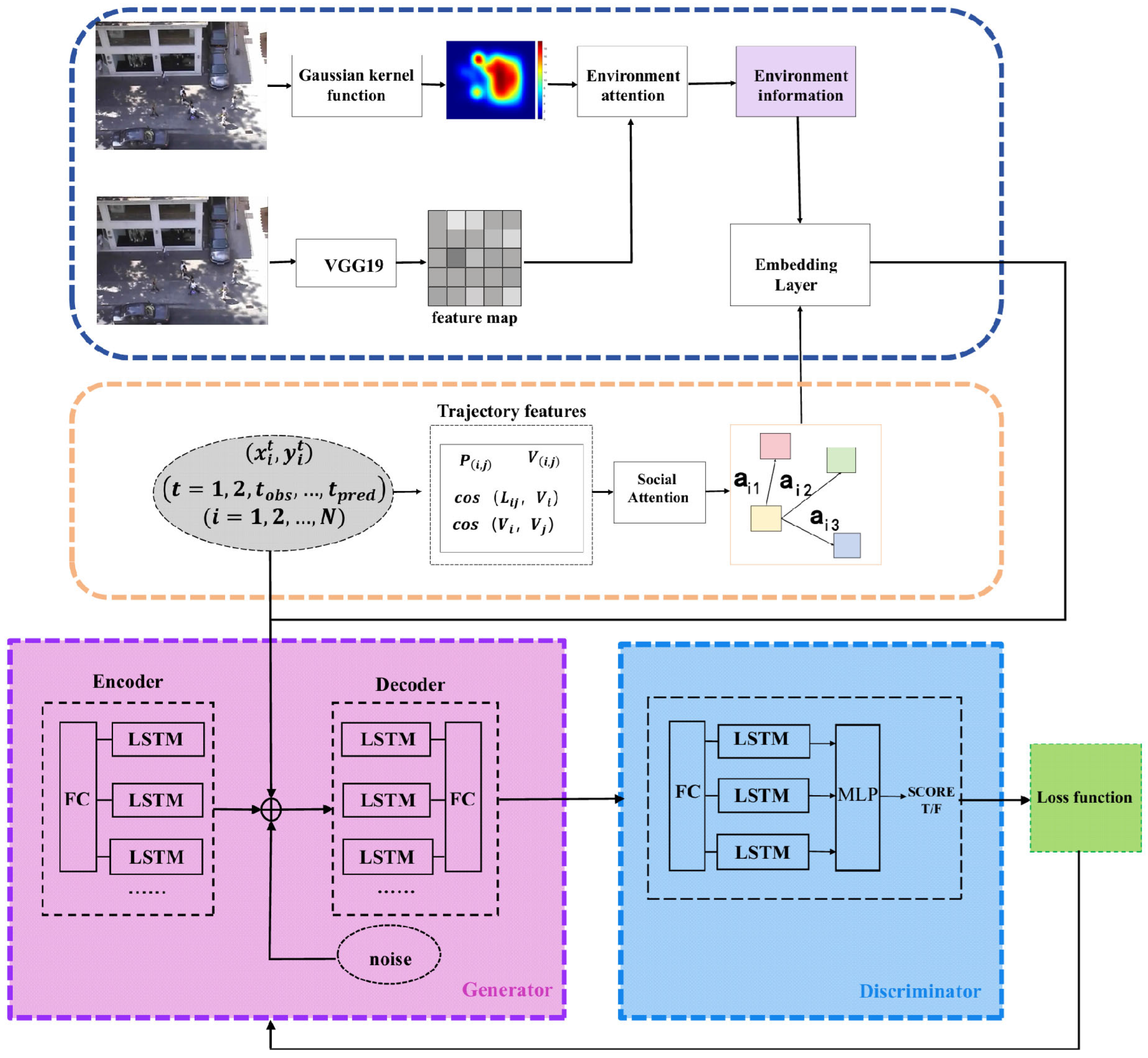
Social Attention Module: This module focuses on pedestrian interaction information and calculates the influence weights of different pedestrians using an attention mechanism. As illustrated in the orange dashed box in Figure 2, this section is used to extract social interaction information of pedestrians. First, four types of interaction information are extracted from the pedestrian trajectories. Then, this interaction information is input into a multi-head attention mechanism to compute the influence weights of different pedestrians and output the comprehensive social interaction information of pedestrians.
Environmental Attention Module: As depicted in the blue dashed box in Figure 2, this module first computes the historical trajectory data of pedestrians using a Gaussian kernel function to obtain the probability density values of different regions. Next, the dataset is transformed into image format, from which feature maps are extracted using a convolutional neural network. The environmental information is then computed from these two types of data within the scene attention module.
Pedestrian Trajectory Prediction Module: As shown in the pink and blue sections of Figure 2, this module predicts pedestrian trajectories using a GAN framework. The GAN consists of two components: the generator and the discriminator. The generator produces future pedestrian trajectory data, while the discriminator evaluates whether the generated trajectories are authentic. The overall model structure is depicted in Figure 2.

3.3. Social Attention Module

From a pedestrian perspective, the target pedestrian’s future trajectory is affected not only by its location x i t , y i t and the last states H i t 1 , but also is significantly affected by the surrounding pedestrians. The target pedestrian is influenced in varying ways by the locations and motion states of nearby pedestrians. If the interactions between each pedestrian and others are not clarified, the trajectory predictions often lack interpretability. Therefore, it is essential to fully extract and utilize the interaction information among pedestrians. We first extract four types of interaction information to characterize the interaction mechanisms among pedestrians. Subsequently, we apply an attention mechanism to calculate the influence weights of nearby pedestrians, allowing the model to focus on information that is more critical for the target pedestrian while minimizing attention to redundant data.

3.3.1. Information Extraction for Pedestrian Interaction Features

The mutual influence of pedestrian interactions is first reconstructed. As illustrated in Figure 3, the future trajectory of the target pedestrian is influenced by the repulsive force, azimuth angle, motion direction angle, and velocity differences of surrounding pedestrians. This research extracts these four interaction features from the ETH and UCY datasets to effectively model pedestrian interactions, thereby fully utilizing the available information.
(1) The repulsive force: According to the pedestrian repulsive force experiment in [20], it represents the maximum measurement value of the skin conductance reaction experiment during pedestrian interaction, which is used to measure the human body pressure. The smaller the reaction time, the greater the pedestrian’s repulsive force.
P i , j = S C R m a x 1 + e k 0 ( r i j L i j s 0 ) , L i j = x i t x j t 2 + y i t y j t 2 1 / 2
where i represents the target pedestrian, j represents the target pedestrian. Their two-dimensional coordinates are x i t , y i t and x j t , y j t . S C R max = 0.283   μ s , k 0 = 95.069   m 1 , and s 0 = 0.007   m . r i j represents the shoulder width of the pedestrian (unit: m), usually 0.35 to 0.45, and the value in this article is 0.4.
(2) Angle of azimuth: Specifically, the angle created by the velocity vector of the target pedestrian i and the displacement vector between pedestrians i and j .
cos L i j , V i = L i j V i L i j × V i = x j t x i t , y i t y i t × x i t x i t 1 , y i t y i t 1 i x j t x i t 2 + y i t y i t 2 1 / 2 × x i t x i t 1 2 + y i t y i t 1 2 1 / 2
(3) Angle of pedestrian movement direction. Specifically, the angle between the target pedestrian i and the pedestrian j ’s motion directions.
cos V i , V j = V i V j V i × V j = x i t x i t - 1 , y i t y i t - 1 × x j t x j t 1 , y j t y j t 1 x i t x i t 1 2 + y i t y i t 1 2 1 / 2 × x j t x j t 1 2 + y j t y j t 1 2 1 / 2
(4) Velocity difference: According to the speed difference, we can judge whether the target pedestrian and the surrounding pedestrians walk together, follow, or surpass.
V i j = V j V i
(5) The four interactions are spliced together to obtain the interaction vector of pedestrian i and pedestrian j at this time t . The interaction information of all the surrounding pedestrians with pedestrian i is aggregated to obtain the social vector θ i t . The expression of the social vector is shown in Equation (5).
θ i t = θ i 1 t , θ i 2 t , θ i 3 t , , θ i N t
where i represents the target pedestrian, j represents the target pedestrian. Their two-dimensional coordinates are x i t , y i t and x j t , y j t . L i j represents the Euclidean distance between pedestrian i and pedestrian j , which is used to calculate the influence of repulsive force on the current motion state of target pedestrian, cos L i j , V i represents the azimuth relationship between two pedestrians, cos V i , V j represents the motion direction relationship between two pedestrians, and V i j represents the difference between the pedestrian i and the pedestrian j on velocity. θ i t represents the social vector of pedestrian i .

3.3.2. Pedestrian Weight Calculation Based on Multiple Attention Mechanism

The attention mechanism, which was developed from research on human vision, significantly enhances performance on tasks requiring the prediction of sequences by identifying relationships between specific sequence components [21]. The attention mechanism can focus on the pedestrian features that are most relevant to the current task, ignoring irrelevant information, and assigning weights to the surrounding pedestrians. This enhances the model’s feature extraction capability and interpretability. This work uses a multi-head attention mechanism [22] to determine the weight of other pedestrians in the context, which is the influence on the target pedestrian i , in order to obtain the influence of surrounding pedestrians on the target pedestrian i . The structure of the attention calculation structure is illustrated in Figure 4 (Figure 4 shows only one of the ‘heads’ of the multi-attention mechanism, and the multi-attention mechanism in this paper has 8 ‘heads’).
As compared to a single-head attention mechanism, a multi-head attention mechanism may learn the dependency of different interaction information more thoroughly through various “heads”, and can subsequently calculate more thoroughly about the influence weight.
Figure 4 depicts the multi-head attention mechanism’s computation procedure. The central idea of the multi-head attention mechanism is to compute the similarity of Q and K T . At time t , our objective is to determine the correlation between the target pedestrian’s state vector H i t and social vector θ i t . After using the attention mechanism to score every single neighbor vector, the influence weight of various neighbor vectors on the trajectory of the target pedestrian is calculated. The calculation formulas of the multi-head attention mechanism are as follows:
θ i t = θ i 1 t , θ i 2 t , , θ i N t , h = 1 , 2 , 3 , 4
f a i ( θ i h t , H i t ) = θ i h t T W a H i t
a i 0 = 𝜕 f a i ( θ i h t , H i t )
C i 0 t = a i 0 H i t
C i t = W O C o n C i 0 t , C i 1 t , C i 2 t , , C i 8 t
This paper designs eight “attention heads” ( h = 8 ), H i t represents the target pedestrian’s state feature vector at the current time, f a represents the scoring function. We then insert the target pedestrian’s state vector H i t and the transformed neighbor vector θ i h t into the attention module, and 𝜕 represents the softmax function, which is used to normalize the scoring results.

3.4. Environment Attention Module

The traditional approach to utilizing environmental information involves extracting scene data through convolutional neural networks. However, this method struggles to effectively demonstrate the potential impact of the environment on individual pedestrians. The presence of obstacles cannot be overlooked; indeed, a large number of pedestrian trajectories reveal certain path preferences. For instance, pedestrians tend to avoid street lamps or uneven road surfaces. Thus, analyzing the distribution of historical trajectory points can provide insights into how the environment influences pedestrian behavior.
In this section, we first employ a Gaussian kernel function to calculate the spatial probability density of different scenes. Next, we utilize the VGG19 model to obtain feature maps of these scenes. Finally, we integrate these two sources of information through an attention mechanism to summarize the environmental factors that warrant greater focus.

3.4.1. Trajectory Density Map

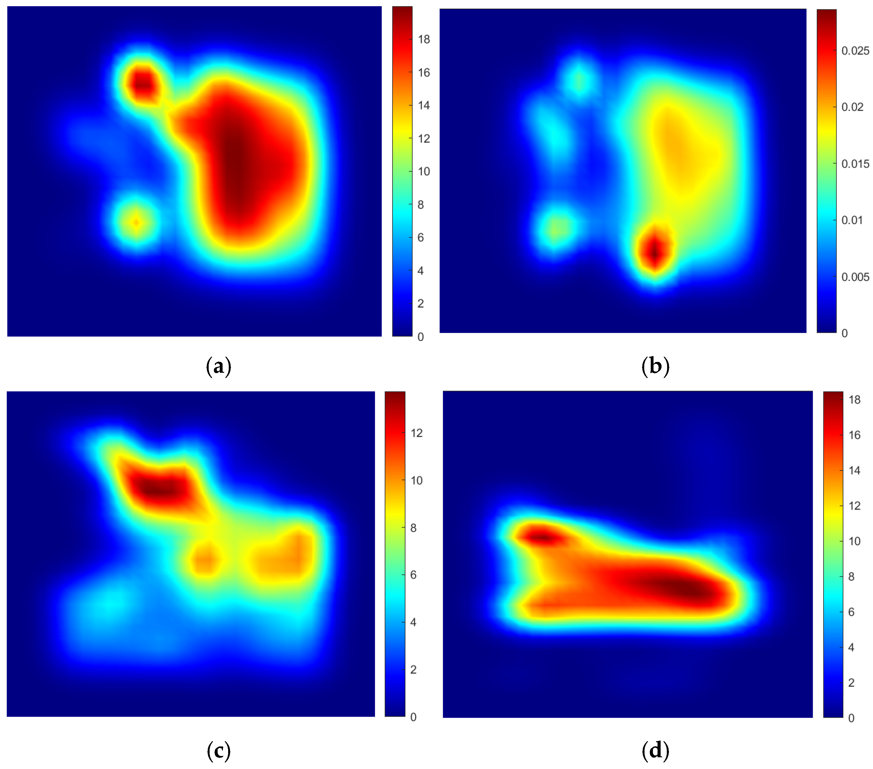
A large amount of pedestrian trajectory data explains the degree of “preference” that pedestrians have for different areas, indicating that the model needs to pay more attention to these areas. This way, we can address the issue that previous work, which only extracts environmental information, cannot establish a connection with pedestrians. In order to obtain the trajectory density values for each spatial location, this paper divides the trajectory data using a Gaussian kernel function based on historical trajectory data, resulting in a trajectory density map for spatial locations in each scene. This trajectory density map illustrates the areas of the congregation for pedestrians within the scene and their certain walking preferences. The Formula (11) for the Gaussian kernel density. Figure 5 shows the spatial probability density feature map of the dataset in this paper.
K ( x i t , y i t ) = e γ x i t y i t 2
where γ is the hyperparameter of the Gaussian kernel function. Coordinates data x i t , y i t is the coordinates of the target pedestrian i .

3.4.2. Scene Semantic Module

As shown in Figure 6, to obtain environmental information, we first extract the scene information using VGG19. Then, we determine the attention levels of pedestrians towards different areas of the scene through spatial probability density values. Finally, we summarize the environmental information that the target pedestrian is focused on using an attention module. We employ pre-trained VGG19 (a network of convolutional neural networks) to extract the features of the scene image so that we may fully utilize the scene information. The pre-trained VGG19 serves as our backbone network, while C i t represents the retrieved characteristics. The scene feature map C i t is shown by Formula (12).
C i t = V G G 19 ( I s c n e , W v g g 19 )
where I s c n e is the processed image data in the dataset, and W v g g 19 is the network parameters of VGG19.
In order to make full use of the scene information, we calculate the scene attention S C i t at each moment t ∈ {1, 2, 3, …, Tobs} according to the scene feature map C i t and the pedestrian trajectory density map K i t . The environment information vector S C i t calculated by scene attention is shown by Formula (13).
S C i t = S c n e A t t ( C i t , K i t , W A t t )
where K i t is the spatial probability density feature map, and W A t t is the network parameters of scene attention.
Figure 6 shows the scene attention module structure.

3.5. Pedestrian Trajectory Prediction

In this paper, pedestrian trajectory prediction is based on a Generative Adversarial Network (GAN) model, which consists of two components: a generator and a discriminator. The generator is responsible for producing the trajectory, while the discriminator’s role is to determine whether the generated trajectory is real or not. The discriminator then provides feedback to the generator through a loss function. The generator encodes and decodes pedestrian trajectories using LSTM. The discriminator classifies the trajectories using LSTM.

3.5.1. The Generator

The generator includes an encoder and a decoder. The encoder takes pedestrian trajectories x i t , y i t as input to obtain the hidden status layer for each pedestrian H i t . The decoder takes H i t , the interaction vector C i t , and the Gaussian noise as input to generate the future trajectory of the target pedestrian.
The generator uses the LSTM as the structure of the encoder and the decoder to learn the neighbor vector of the historical trajectory, encode the historical trajectory, decode the neighbor vector, and, finally, obtain the predicted future trajectory.
The calculation formula of the encoder can be expressed as
S i t = F e ( C i t , S C i t , W F e )
τ i = f 1 x i t , y i t ; w f 1
H i t = L S T M H i t 1 , τ i ; ω g 1
where S i t represents the unification of pedestrian interaction information and environmental information in the embedding layer. x i t , y i t is the position for pedestrians i at the moment t , f 1 is a fully connected network, w f 1 is the parameter of the fully connected network, τ i is the pedestrian track feature vector at the current time, H i t is the pedestrian track feature vector at the current time, and ω g 1 is the weight parameter in the LSTM neural network layer.
The neighbor vector of the pedestrian at this moment and the state vector of the last moment of the trajectory data are spliced and input into the decoder to predict the trajectory of the pedestrian at the next moment.
The calculation formula of the decoder can be expressed as
C o n i t + 1 = [ f 2 ( S i t , H i t ; W f 2 ) , z ]
H i t + 1 = L S T M C o n i t , H i t ; W g 2
x i t + 1 , y i t + 1 = f 3 H i t + 1 ; W f 3
where z is Gaussian noise, f 2 and f 3 are the fully connected networks, W f 2 and W f 3 are, respectively, the weight parameters of the fully connected networks, W g 2 is the weight parameter of the LSTM network, M is a fully connected network, W M is the parameter of the fully connected network, H i t is the hidden state of the target pedestrian, H i t and the C o n i t are input into the LSTM to obtain the next state H i t + 1 of the target pedestrian. Then, the H i t + 1 is input into the fully connected network to obtain the predicted trajectory coordinates x i t + 1 , y i t + 1 .

3.5.2. The Discriminator

The purpose of the discriminator is to determine whether the input data is real data from the database or generated data from the generator, and both types of data are represented by T r a j i . The discriminator first transforms the two types of trajectories from coordinate space to feature space to obtain U i t , then uses LSTM to keep updating the final state H f i n t , and, finally, scores the final moment state by multiple perceptron and softmax classifier to tell if the trajectory is true or false, and passes it to the generator by back propagation to promote the generator to generate more accurate trajectories.
U i t = f 4 ( T r a j i ; W f 4 )
H f i n t + 1 = L S T M ( H f i n t , U i t ; W f i n )
S f i n i = f D ( h f i n t + 1 ; W f D )
where f 4 is the fully connected network, H f i n t is the movement state of the target pedestrian at the last moment, and W f i n is the network parameter of LSTM, f D is the multiple perceptron, W f D is the parameter of the multiple perceptron, and S f i n i is the final score of the trajectory.

3.5.3. The Loss Function

The loss function in this paper consists of two parts, including L GAN and L 2 , the specific formulas are as follows:
L = L G A N G , D + J L L 2 G
L G A N G , D = min G   max D E T i   ~   p d a t e x i , y i [ log D U i ] + E z ~ p z log 1 D G x i , z
L L 2 G = min k Y i G x i , z k 2
where L is the loss function of the model, L G A N ( G , D ) is the loss function of the Generative Adversarial Network, L L 2 G is used to calculate the difference between the generated trajectory and the true trajectory, and encourage the generator to generate more realistic and socially conforming trajectory samples as much as possible, m a x D represents updating the arguments of the discriminator by maximizing the L L 2 with the generator fixed, m i n G represents that the generator minimizes L L 2 when the discriminator maximizes L L 2 , which is essentially a cross entropy, and ϑ is the hyperparameter. E is the expected value calculated for the model. The ultimate purpose of the discriminator is to keep D U i approaching 1 and D G x i , z approaching 0.

4. Experiment and Analysis

4.1. Datasets

Experiments were conducted on two public pedestrian trajectory prediction datasets—ETH [1] and UCY [23]—which include five social scenarios. The ETH dataset comprises two scenarios, ETH and hotel, while the UCY dataset includes three scenarios, Univ, zara1, and zara2. Both datasets provide a wealth of pedestrian trajectory information and diverse scenarios, encompassing approximately 1536 pedestrians in total. The ETH dataset primarily captures the walking patterns of pedestrians in relatively busy public spaces, such as squares and sidewalks. In contrast, the UCY dataset covers a broader range of environments, including shopping malls and city streets, and features various types of pedestrian interactions, such as avoidance, following, and group walking.
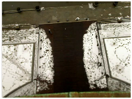
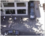
Together, these datasets offer extensive data on pedestrian interactions and encompass rich scenarios, including densely populated shopping areas and transit stations with high pedestrian flow. This makes them particularly suitable for studying both pedestrian interactions and pedestrian–environment interactions, as explored in this paper. The scenes contained in the ETH and UCY datasets are summarized in Table 1. In the ETH dataset, Site 1 refers to the ETH dataset scene, where pedestrian density is low, but there are frequent interactions between pedestrians and static obstacles. Site 2 refers to the hotel dataset scene, where pedestrians primarily walk in a straight line. In the UCY dataset, Site 1 corresponds to the Zara dataset scene, characterized by a high pedestrian density, the presence of stationary crowds, and numerous pedestrian interactions. Site 2 refers to the Univ dataset scene, which features a high pedestrian density, slow-moving crowds, and obstacles such as streetlights and flower beds.

4.2. Experimental Details

The experiment was conducted using the Windows 10 operating system, with the deep learning framework Pytorch 1.8.1, CUDA 10.2, and cuDNN 7.6.5 installed, as well as an Intel Core i7-10700K CPU and an NVIDIA Quadro RTX5000 GPU. The learning rate of the trajectory generator is 0.0005, and the learning rate of the trajectory discriminator is 0.001, using the Adam algorithm optimizer, t o b s = 8 , t p r e d = 12 . This model uses the cross-validation method for its training and testing processes. We select four of these datasets as the training set and the remaining dataset as the test dataset.
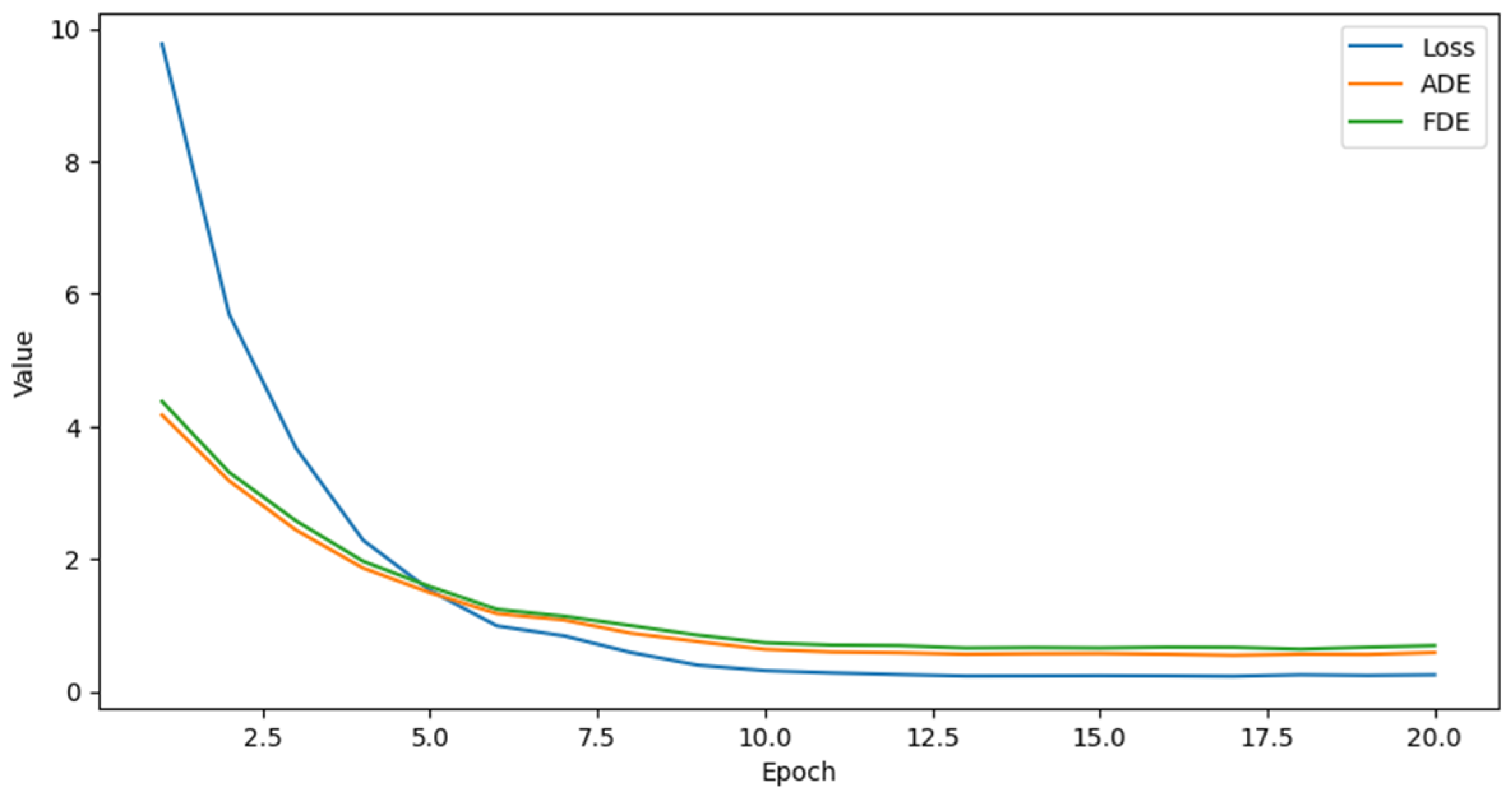
Figure 7 illustrates the training process of the model using the training dataset. It is evident that the model’s loss function decreases as the number of epochs increases, eventually leveling off. Throughout this process, both the Average Displacement Error (ADE) and Final Displacement Error (FDE) metrics also stabilize alongside the loss value. This indicates that the model is learning and adjusting its parameters to make its predictions closer to the true values to gradually reduce the prediction error of the trajectory.

4.3. Metrics

We use the Average Displacement Error (ADE) and the Final Displacement Error (FDE) as evaluation metrics.
(1) Average Displacement Error (ADE) refers to the mean square error of all predicted trajectory points and real trajectory points. ADE was defined as
A D E i = 1 T t = 1 T x i t x ~ i t 2 + y i t y ~ i t 2 1 / 2 , A D E = 1 N t = 1 T A D E i
(2) Final Displacement Error (FDE) refers to the distance between the predicted trajectory of the endpoint and the actual trajectory of the endpoint. FDE was defined as
F D E i = x i T x ~ i T 2 + y i T y ~ i T 2 1 / 2 , F D E = 1 N i = 1 N F D E i

4.4. Analysis of Results

4.4.1. Quantitative Results

In this study, classical trajectory prediction models including SGC-LSTM [24], S-LSTM [3], Sophie [13], and S-GAN are selected and compared with the SISGAN model. Table 2 presents the comparative findings of the Average Displacement Error (ADE) and Final Displacement Error (FDE) for each method, with measurements expressed in meters. Each row details the prediction error of each model across various dataset scenarios. Notably, the accuracy of the model’s predictions is inversely correlated with the magnitude of the prediction error reflected in the table.
To provide a clearer representation of the variability among the different results, we have converted the prediction errors from Table 2 into a bar chart, as shown in Figure 8, and will analyze them in detail.
As illustrated in Figure 8, pedestrian trajectory prediction models based on Generative Adversarial Networks (GANs) generally outperform those based on Long Short-term Memory (LSTM) networks. This superior performance is primarily due to the adversarial training between the discriminator and generator in GAN-based approaches, which continuously enhances prediction capabilities.
A comparison of the prediction performance among the SGAN, Sophie, and SISGAN models reveals that those who effectively learn both pedestrian interactions and environmental data yield more accurate predictions. In the case of the hotel dataset, which predominantly features linear pedestrian trajectories, the SGC-LSTM model surpasses the SISGAN model proposed in this thesis. The SISGAN model, with its social attention and environmental information modules, possesses a more complex network structure, which can lead to decreased accuracy in simpler scenarios.
Conversely, for datasets such as ETH, Univ, and Zara, which include intricate pedestrian interactions and numerous static obstacles, the SISGAN model demonstrates superior predictive performance. This highlights the effectiveness of the SISGAN model in emphasizing pedestrian interactions and assimilating scene information.

4.4.2. Qualitative Results

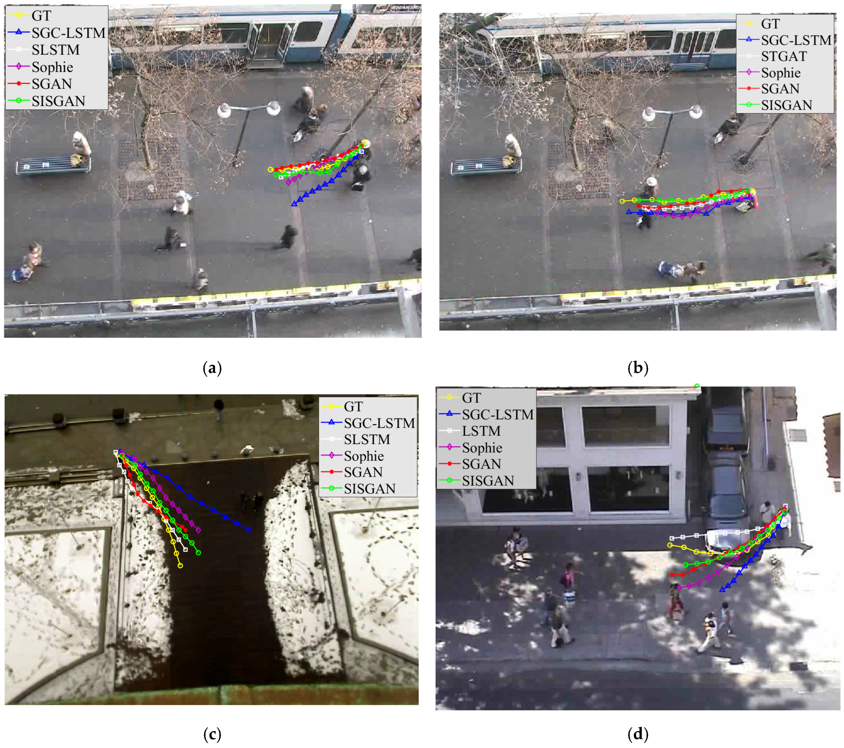
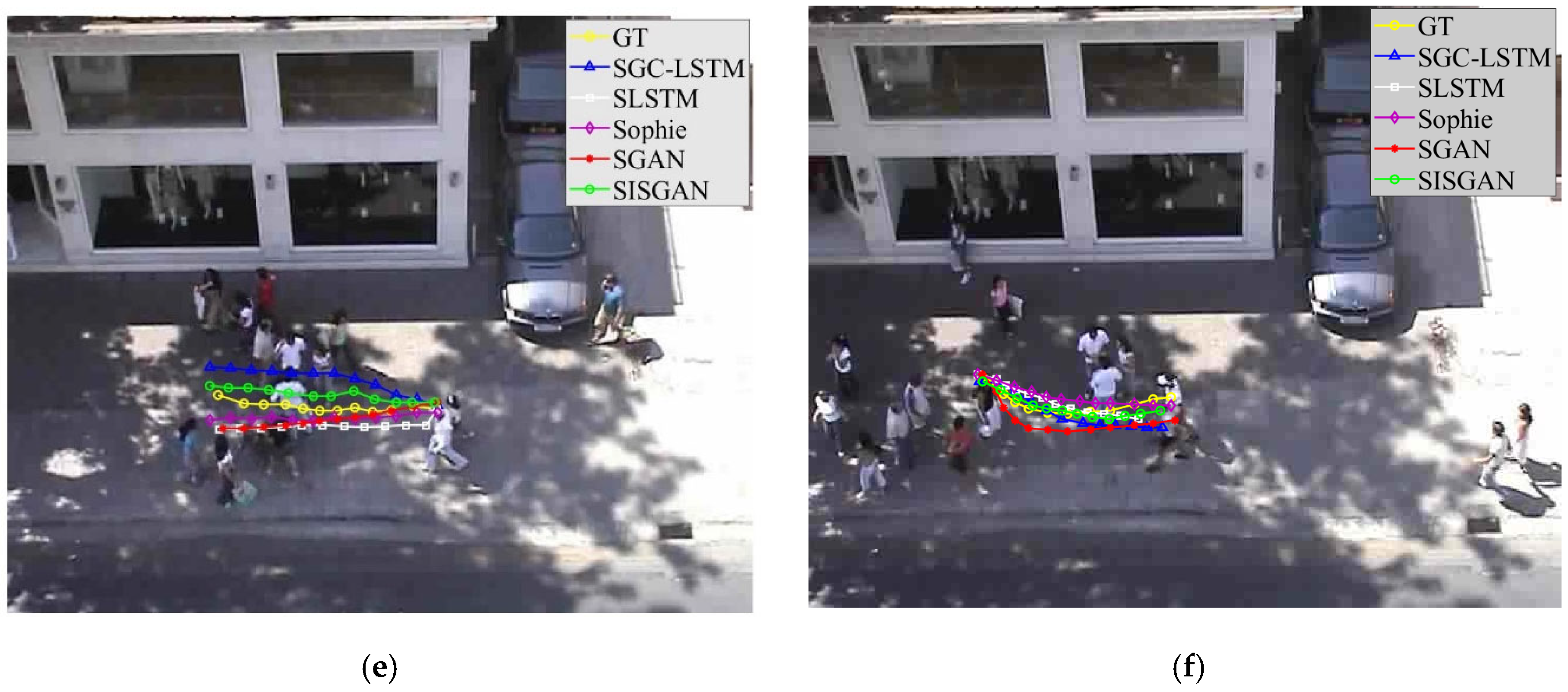
We selected and visualized the prediction data for six scenarios, as illustrated in Figure 9. To provide a more intuitive representation of the model’s predictive performance, we simultaneously visualized the prediction data for real trajectories alongside those generated by SGC-LSTM, S-LSTM, Sophie, and S-GAN. In our experiments, the historical trajectory data step was set to 8, while the prediction step encompassed 12 time steps, with each time step representing 0.4 s. In scenarios featuring sparse individual flows, panels (a) and (b) demonstrate the model’s predictive capabilities. In this context, the predictions generated by the SISGAN model prove to be quite accurate. Notably, in panel (a), the SISGAN’s attention module effectively captures interactive data concerning the target pedestrian’s left side and the tree on their right, resulting in prediction outputs that closely align with the real trajectory. Panel (c) depicts the target pedestrians walking along the edge of the snow, where only the SISGAN model predicts a trajectory that successfully avoids the snow. This outcome is attributed to the SISGAN scenario module, which employs CNN to map spatial probability density to the semantic information within the region. In panel (d), the pedestrian navigates around a car before continuing along the path. Although some errors occur, the SISGAN model effectively captures the pedestrian’s walking intentions. Panels (e) and (f) illustrate scenarios involving dense crowds. In panel (e), while predictions from all models exhibit deviations, the SISGAN model’s predictions successfully navigate around pedestrians on both sides, making them the closest to the ground truth.

4.4.3. Results of Ablation Experiments

To validate the effectiveness of the social attention module and the scene information module, we conducted experiments by removing both modules from the original model. Table 3 presents the comparative results of Average Displacement Error (ADE) and Final Displacement Error (FDE) for models with different configurations, while Figure 10 visualizes the results of the ablation experiment.
In this paper, we selected the following three models for comparison: the SGAN model, which does not utilize pedestrian interaction information for predictions; the SIGAN model, which employs only the interaction attention module; and the SISGAN model, which simultaneously uses both the interaction attention module and the environmental information module. This comparison is intended to validate the effectiveness of the proposed interaction attention module and environmental information module. The results of the ablation experiments are presented in Table 3.
From Table 3, it is evident that the overall prediction performance of the SIGAN model is better than that of the SGAN model. However, the prediction results of the SIGAN model on the ETH dataset are inferior to those of the SGAN model. This discrepancy can be attributed to the complexity introduced by the extensive calculations of pedestrian interactions within the SIGAN model. The ETH dataset contains a significant number of static obstacles but a relatively low pedestrian density, which leads to the complex network model actually degrading trajectory prediction performance. Additionally, we observe that the SISGAN model demonstrates improved prediction results compared to the SIGAN model, particularly in the Univ and zara2 datasets, which feature a greater presence of static and dynamic obstacles. These results confirm the effectiveness of the interaction attention module and environmental information module designed in this paper.
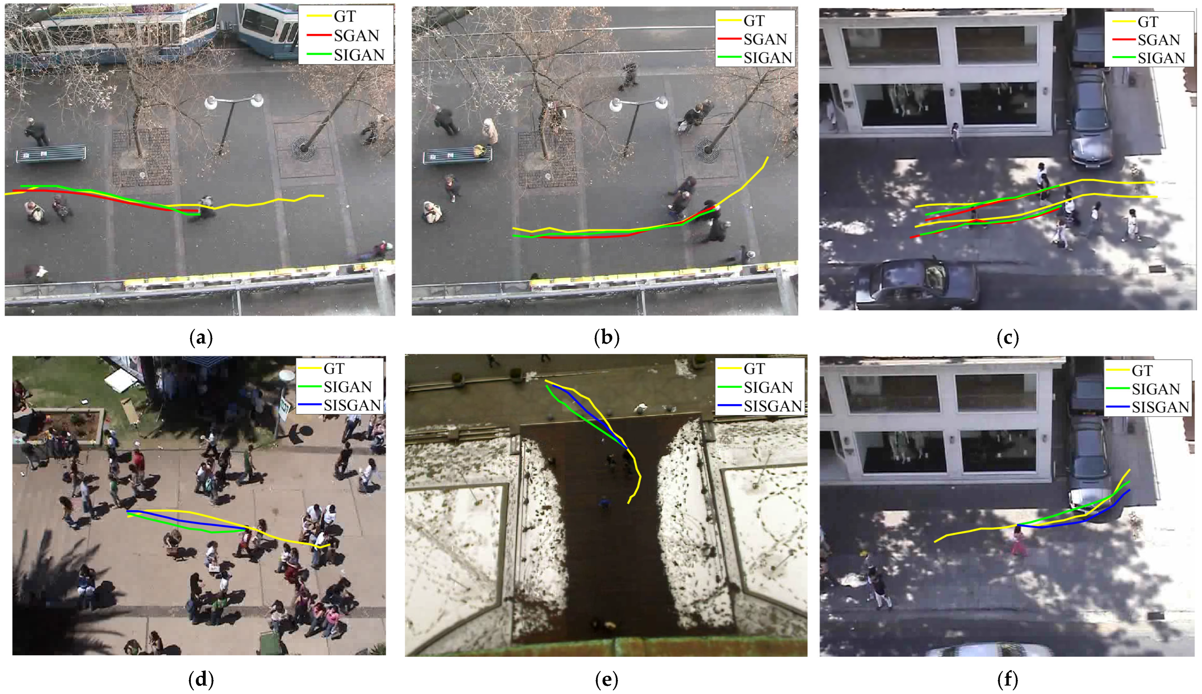
As illustrated in Figure 10, panel (a) shows the movement of pedestrians avoiding those in front of them. It is evident that the SIGAN model presented in this paper demonstrates a more pronounced ability to avoid pedestrians compared to the SGAN model. Panel (b) indicates that the trajectory predictions from both the SGAN and SIGAN models are largely similar in sparse scenarios. In panel (c), we observe that the SIGAN model yields relatively smaller errors in companion situations. Panel (d) highlights that, while there are no significantly large errors in the final predicted positions, the prediction process itself does not achieve the desired accuracy. Panels (e) and (f) illustrate that the SISGAN model, which incorporates the environmental information module, provides superior trajectory data for obstacle avoidance compared to the SIGAN model does not emphasize environmental context, particularly in situations where obstacles need to be navigated or when pedestrians are walking alongside them.
We believe that the ablation experiments validate the effectiveness of both the social interaction module and the environmental information module in this study. However, due to the independence of individual pedestrians, even though the model can predict the final locations of pedestrians more accurately, there is still a need for the model to better understand pedestrians’ walking intentions. This understanding would enhance the accuracy of trajectory predictions.

5. Conclusions

In this work, we propose a pedestrian trajectory prediction method that effectively integrates social interactions and environmental information. Our approach extracts four types of interaction data and calculates influence weights for different pedestrians from their perspectives. This addresses the limitations of previous studies that primarily focused on pedestrian interactions based on distance or velocity. Furthermore, we establish potential correlations between desired pedestrian scenes by utilizing historical trajectory density distributions, enabling a more targeted extraction of scene information. We conduct experiments on the ETH and UCY datasets to demonstrate the effectiveness of each component of our approach. However, the pedestrian trajectory prediction method proposed in this paper uses an attention mechanism to calculate the impact weights of interaction features and environmental information features. The computation process of the attention mechanism generates a large number of matrix operations and fully connected layer calculations, which increases the computation time and cost. In the future, we aim to design a sliding window to extract regional information surrounding the pedestrian, including a controllable scene information range and a manageable number of surrounding pedestrians. For example, in densely populated areas, a smaller window can be chosen to capture details, while in open areas, a larger window can be used to obtain more contextual information. This dynamic control approach reduces redundant calculations of other information and improves the computational efficiency of the model.

Author Contributions

Conceptualization, L.L. and W.D.; methodology, W.D.; software, W.D.; validation, L.L. and W.D.; formal analysis, W.D.; resources, L.L.; data curation, W.D.; writing—original draft preparation, W.D.; writing—review and editing, L.L.; visualization, W.D.; supervision, L.L. All authors have read and agreed to the published version of the manuscript.

Funding

This research received no external funding.

Institutional Review Board Statement

Not applicable.

Informed Consent Statement

Not applicable.

Data Availability Statement

The datasets presented in this article are not readily available because the data are part of an ongoing study. Requests to access the datasets should be directed to [email protected].

Conflicts of Interest

The authors declare no conflict of interest.

References

  1. Helbing, D.; Molnar, P. Social force model for pedestrian dynamics. Phys. Rev. E Stat. Phys. Plasmas Fluids Relat. Interdiscip. Top. 1995, 51, 4282–4286. [Google Scholar] [CrossRef] [PubMed]
  2. Pellegrini, S.; Ess, A.; Schindler, K.; van Gool, L. You’ll never walk alone: Modeling social behavior for multi-target tracking. In Proceedings of the 2009 IEEE 12th International Conference on Computer Vision (ICCV), Kyoto, Japan, 29 September–2 October 2009; pp. 261–268. [Google Scholar]
  3. Alahi, A.; Goel, K.; Ramanathan, V.; Robicquet, A.; Fei-Fei, L.; Savarese, S. Social LSTM: Human Trajectory Prediction in Crowded Spaces. In Proceedings of the 29th IEEE Conference on Computer Vision and Pattern Recognition, Las Vegas, NV, USA, 26 June–1 July 2016; pp. 961–971. [Google Scholar] [CrossRef]
  4. Xu, K.; Qin, Z.; Wang, G.; Huang, K.; Ye, S.; Zhang, H. Collision-Free LSTM for Human Trajectory Prediction. In Proceedings of the MultiMedia Modeling: 24th International Conference, MMM 2018, Bangkok, Thailand, 5–7 February 2018; Springer: Berlin/Heidelberg, Germany, 2018; pp. 106–116. [Google Scholar] [CrossRef]
  5. Haddad, S.; Wu, M.; Wei, H.; Lam, S.K. Situation-Aware Pedestrian Trajectory Prediction with Spatio-Temporal Attention Model. In Proceedings of the 24th Computer Vision Winter Workshop Friedrich Fraundorfer, Stift Vorau, Austria, 6–8 February 2019; Volume 25, pp. 4–13. [Google Scholar] [CrossRef]
  6. Kim, S.; Chi, H.-G.; Lim, H.; Ramani, K.; Kim, J.; Kim, S. Higher-order Relational Reasoning for Pedestrian Trajectory Prediction. In Proceedings of the 2024 IEEE/CVF Conference on Computer Vision and Pattern Recognition (CVPR), Seattle, WA, USA, 16–22 June 2024; pp. 15251–15260. [Google Scholar]
  7. Su, Y.; Li, Y.; Wang, W.; Zhou, J.; Li, X. A Unified Environmental Network for Pedestrian Trajectory Prediction. Proc. AAAI Conf. Artif. Intell. 2024, 38, 4970–4978. [Google Scholar] [CrossRef]
  8. Cheng, H.; Liu, M.; Chen, L.; Broszio, H.; Sester, M.; Yang, M.Y. GATraj: A graph- and attention-based multi-agent trajectory prediction model. ISPRS J. Photogramm. Remote Sens. 2023, 205, 163–175. [Google Scholar] [CrossRef]
  9. Giuliari, F.; Hasan, I.; Cristani, M.; Galasso, F. Transformer Networks for Trajectory Forecasting. In Proceedings of the 2020 25th International Conference on Pattern Recognition (ICPR), Milan, Italy, 10–15 January 2021; pp. 10335–10342. [Google Scholar]
  10. Chen, X.; Zhang, H.; Hu, Y.; Liang, J.; Wang, H. VNAGT: Variational Non-Autoregressive Graph Transformer Network for Multi-Agent Trajectory Prediction. IEEE Trans. Veh. Technol. 2023, 72, 12540–12552. [Google Scholar] [CrossRef]
  11. Czech, P.; Braun, M.; Kreßel, U.; Yang, B. On-Board Pedestrian Trajectory Prediction Using Behavioral Features. In Proceedings of the 2022 21st IEEE International Conference on Machine Learning and Applications (ICMLA), Nassau, Bahamas, 12–14 December 2022; Volume 48, pp. 437–443. [Google Scholar]
  12. Wang, J.; Sang, H.; Chen, W.; Zhao, Z. VOSTN: Variational One-Shot Transformer Network for Pedestrian Trajectory Prediction. Phys. Scr. 2024, 99, 026002. [Google Scholar] [CrossRef]
  13. Sadeghian, A.; Kosaraju, V.; Hirose, N.; Rezatofighi, H.; Savarese, S. SoPhie: An Attentive GAN for Predicting Paths Compliant to Social and Physical Constraints. In Proceedings of the 2019 IEEE/CVF Conference on Computer Vision and Pattern Recognition (CVPR), Long Beach, CA, USA, 15–20 June 2019; pp. 1349–1358. [Google Scholar]
  14. Lai, W.-C.; Xia, Z.-X.; Lin, H.-S.; Hsu, L.-F.; Shuai, H.-H.; Jhuo, I.-H.; Cheng, W.-H. Trajectory Prediction in Heterogeneous Environment via Attended Ecology Embedding. In Proceedings of the MM ‘20: The 28th ACM International Conference on Multimedia, Seattle, WA, USA, 12–16 October 2020. [Google Scholar]
  15. Xue, H.; Huynh, D.Q.; Reynolds, M. SS-LSTM: A Hierarchical LSTM Model for Pedestrian Trajectory Prediction. In Proceedings of the 2018 IEEE Winter Conference on Applications of Computer Vision (WACV), Lake Tahoe, NV, USA, 12–15 March 2018; pp. 1186–1194. [Google Scholar]
  16. Manh, H.; Alaghband, G. Scene-LSTM: A Model for Human Trajectory Prediction. arXiv 2019. [Google Scholar] [CrossRef]
  17. Syed, A.; Morris, B.T. SSeg-LSTM: Semantic Scene Segmentation for Trajectory Prediction. In Proceedings of the 2019 IEEE Intelligent Vehicles Symposium (IV), Paris, France, 9–12 June 2019; pp. 2504–2509. [Google Scholar]
  18. Chen, W.; Sang, H.; Wang, J.; Zhao, Z. WTGCN: Wavelet transform graph convolution network for pedestrian trajectory prediction. Int. J. Mach. Learn. Cybern. 2024, 1–18. [Google Scholar] [CrossRef]
  19. Kosaraju, V.; Sadeghian, A.; Martín-Martín, R.; Reid, I.; Rezatofighi, H.; Savarese, S. Social-BiGAT: Multimodal Trajectory Forecasting using Bicycle-GAN and Graph Attention Networks. Adv. Neural Inf. Process. Syst. 2019, 137–146. [Google Scholar] [CrossRef]
  20. Zhao, Y.; Lu, T.; Su, W.; Wu, P.; Fu, L.; Li, M. Quantitative measurement of social repulsive force in pedestrian movements based on physiological responses. Transp. Res. Part B Methodol. 2019, 130, 1–20. [Google Scholar] [CrossRef]
  21. Vaswani, A. Attention is all you need. Advances in Neural Information Processing Systems. arXiv 2017. [Google Scholar] [CrossRef]
  22. Bolya, D.; Fu, C.Y.; Dai, X.; Zhang, P.; Hoffman, J. Hydra attention: Efficient attention with many heads. In Proceedings of the Computer Vision–ECCV 2022 Work Shops, Tel Aviv, Israel, 23–27 October 2022; Springer Nature: Cham, Switzerland, 2023; pp. 35–49. [Google Scholar] [CrossRef]
  23. Lerner, A.; Chrysanthou, Y.; Lischinski, D. Crowds by Example. Comput. Graph. Forum 2007, 26, 655–664. [Google Scholar] [CrossRef]
  24. Zhou, Y.; Wu, H.; Cheng, H.; Qi, K.; Hu, K.; Kang, C.; Zheng, J. Social graph convolutional LSTM for pedestrian trajectory prediction. IET Intell. Transp. Syst. 2021, 15, 396–405. [Google Scholar] [CrossRef]
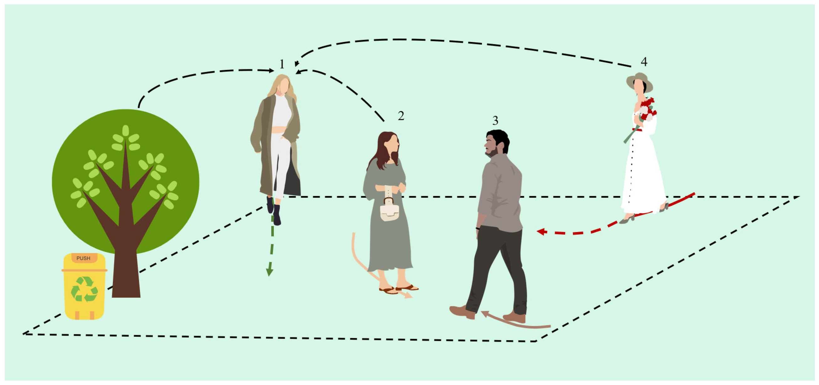
Figure 1. Pedestrian interaction scenario portrayal. Pedestrian 1 observes the surrounding pedestrians and other physical environments while walking. Whether it is a static crowd, like pedestrians 2 and 3, or pedestrian 4 walking in the opposite direction, these factors will influence pedestrian 1 to continuously adjust their trajectory.
Applsci 14 09537 g001
Figure 2. Network structure of SIS-GAN model. The upper blue dashed section represents the environmental information module, and the middle orange dashed section represents the interaction attention module. The bottom is a GAN-based trajectory prediction framework, where the historical trajectory information of pedestrians and the auxiliary information from the previous two sections are input into the decoder to predict pedestrian trajectories. The discriminator scores the generated trajectories, and the loss derived from these scores is returned to the generator, incentivizing it to continuously generate more realistic trajectories.
Applsci 14 09537 g002
Figure 3. Description of pedestrian interaction. To characterize the interactive effects between pedestrians, this paper first extracts information related to pedestrian movement based on pedestrian kinematics: the position, speed, direction of movement, and repulsive forces of pedestrians. The position information of pedestrians is taken with the bottom left corner of each scene as the origin of the coordinate system. Then, based on the pedestrian’s position information and their position in the next second, the speed, direction of movement, and repulsive force of the pedestrian are calculated.
Applsci 14 09537 g003
Figure 4. Schematic diagram of attention mechanism. To calculate the influence weights between pedestrians, this paper first computes the similarity between the target pedestrian’s historical states H i t and the social vectors θ i t with other pedestrians, deriving the influence weights for different pedestrians. All interaction information is then consolidated into the target pedestrian’s social information C i 0 t . In the figure, the blue squares and pink squares represent the information after H i t and θ i t are processed linearly, respectively.
Applsci 14 09537 g004
Figure 5. Spatial probability density map, where (a) is the scenario from the ETH dataset, (b) the scenario from the hotel dataset, (c) the scenario from the zara1 dataset, and (d) the scenario from the zara2 dataset. The thermal bar scale on the right side of the figure represents the density of trajectories in different regions of the scenario. The coordinate origin of these four images is at the bottom left corner. The different density values reflect the density of pedestrian historical trajectories in various areas of the scene and indicate the level of “preference” pedestrians have for different regions. When the density value of a particular area is high, the model needs to focus on the pedestrian density and trajectory distribution within that area to avoid predicting trajectories that result in “collisions”.
Applsci 14 09537 g005
Figure 6. Scene attention module structure. First, the spatial probability density map and the scene feature map are aligned through the FC layer, then input into the attention mechanism to compute the influence weights of different regions, and output the scene information for that particular scene.
Applsci 14 09537 g006
Figure 7. The results of the SISGAN model on the training datasets in terms of loss, ADE, and FDE metrics during the training process. The x-axis represents the number of epochs of training, and the y-axis represents the loss value during model training increases.
Applsci 14 09537 g007
Figure 8. Experimental results of different methods. We present the results of different models on all datasets from ETH and UCY in the form of a bar chart. The X-axis represents different trajectory prediction methods, while the Y-axis shows the prediction error of each method across all datasets, with the unit in meters. (a) The Average Displacement Error (ADE) of different methods on ETH and UCY. (b) The Final Displacement Error (FDE) of different methods on ETH and UCY.
Applsci 14 09537 g008
Figure 9. Comparison of trajectory prediction of different models, where (a,b) are from the hotel dataset, (c) is from the ETH dataset, (d) is from the zara1 dataset, and (e,f) are from the zara2 dataset. (a) shows pedestrians avoiding obstacles on both sides; (b) shows pedestrians’ trajectories in a sparse scene; (c) shows pedestrians avoiding snow; (d) shows pedestrians walking along the edges of a car; (e) shows pedestrians adjusting their paths in the face of a stationary, dense crowd to avoid a collision; and (f) shows pedestrians avoiding oncoming pedestrians.
Applsci 14 09537 g009aApplsci 14 09537 g009b
Figure 10. Comparison of trajectory prediction of ablation study, where (a,b) are from the hotel dataset, (c) from the zara1 dataset, (d) from the Univ dataset, (e) from the ETH dataset, and (f) from the zara2 dataset. (a) shows pedestrians avoiding stationary pedestrians; (b) shows pedestrians avoiding pedestrians on both sides; (c) shows pedestrians walking in pairs; (d) shows pedestrians walking around stationary obstacles; (e) shows pedestrians adjusting their paths in the face of a dense crowd to avoid a collision; and (f) shows pedestrians walking along the edges of a car.
Applsci 14 09537 g010
Table 1. ETH and UCY scenes.
DatasetsSite 1Site 2
ETHApplsci 14 09537 i001Applsci 14 09537 i002
UCYApplsci 14 09537 i003Applsci 14 09537 i004
Table 2. The Average Displacement Error (ADE) and Final Displacement Error (FDE) of different methods on ETH and UCY.
DatasetADE/FDE (Meter)
SGC-LSTMSLSTMSophieSGANSISGAN
ETH0.82/1.721.09/2.350.70/1.430.67/1.130.63/0.95
hotel0.45/0.650.79/1.760.76/1.670.72/1.610.58/1.62
Univ0.53/1.100.67/1.400.54/1.240.61/1.280.50/1.10
zara10.40/0.920.47/1.000.30/0.630.34/0.710.31/0.68
zara20.36/0.780.56/1.170.38/0.780.42/0.840.30/0.73
Average0.51/1.030.72/1.540.54/1.150.58/1.190.46/1.01
Note: the bold data in the table are the best results predicted by the model.
Table 3. The Average Displacement Error (ADE) and Final Displacement Error (FDE) of models with different modules on ETH and UCY.
DatasetADE/FDE (Meter)
SGANSIGANSISGAN
ETH0.67/1.130.79/1.430.63/0.95
hotel0.72/1.610.58/1.210.58/1.62
Univ0.61/1.280.65/1.410.50/1.10
zara10.34/0.710.32/0.800.31/0.68
zara20.42/0.840.42/0.780.30/0.73
Average0.58/1.190.51/1.100.46/1.01
Note: the bold data in the table are the best results predicted by the model.
Disclaimer/Publisher’s Note: The statements, opinions and data contained in all publications are solely those of the individual author(s) and contributor(s) and not of MDPI and/or the editor(s). MDPI and/or the editor(s) disclaim responsibility for any injury to people or property resulting from any ideas, methods, instructions or products referred to in the content.