Article

Reduced-Order Modeling for Dynamic System Identification with Lumped and Distributed Parameters via Receptance Coupling Using Frequency-Based Substructuring (FBS)

by
Behzad Hamedi
1,* and
Saied Taheri
2
1
Engineering Mechanics Program, Mechanical Engineering Department, Virginia Polytechnic Institute and State University, Blacksburg, VA 24061, USA
2
Center for Tire Research (CenTiRe), Mechanical Engineering Department, Virginia Polytechnic Institute and State University, Blacksburg, VA 24061, USA
*
Author to whom correspondence should be addressed.
Appl. Sci. 2024, 14(20), 9550; https://doi.org/10.3390/app14209550
Submission received: 4 September 2024 / Revised: 13 October 2024 / Accepted: 18 October 2024 / Published: 19 October 2024
(This article belongs to the Special Issue Nonlinear Dynamics and Vibration)

Abstract

:
Paper presents an effective technique for developing reduced-order models to predict the dynamic responses of systems using the receptance coupling and frequency-based substructuring (RCFBS) method. The proposed approach is particularly suited for reconfigurable dynamic systems across various applications, like cars, robots, mechanical machineries, and aerospace structures. The methodology focuses on determining the overall system receptance matrix by coupling the receptance matrices (FRFs) of individual subsystems in a disassembled configuration. Two case studies, one with distributed parameters and the other with lumped parameters, are used to illustrate the application of this approach. The first case involves coupling three substructures with flexible components under fixed–fixed boundary conditions, while the second case examines the coupling of subsystems characterized by multiple masses, springs, and dampers, with various internal and connection degrees of freedom. The accuracy of the proposed method is validated against a numerical finite element analysis (FEA), direct methods, and a modal analysis. The results demonstrate the reliability of RCFBS in predicting dynamic responses for reconfigurable systems, offering an efficient framework for reduced-order modeling by focusing on critical points of interest without the need to account for detailed modeling with numerous degrees of freedom.

1. Introduction

Modeling dynamic systems with both continuous or lumped characteristics presents significant challenges, particularly as the number of degrees of freedom (DoFs) increases when both rotational and translational DoFs are involved. These challenges are further compounded by the presence of constraints and boundary conditions, which affect the system’s dynamic behavior. To address these complexities, a reduced-order modeling approach is essential, offering a practical alternative for predicting system responses without requiring detailed, resource-intensive modeling as a backup and effective solution. This approach provides a balance between accuracy and computational efficiency, making it feasible to handle even highly complex systems. To develop an effective reduced-order model with hybrid and modular capabilities, receptance coupling frequency-based substructuring (RCFBS) offers a robust framework for predicting system responses. RCFBS combines subsystem receptance matrices, enabling reliable predictions of the system’s dynamic behavior across a specific frequency range, particularly in regions where the system behaves linearly. This methodology is highly beneficial for engineers, especially during early product development phases, when constructing a full vehicle finite element model (FEM) or multi-body dynamic model (MBD) may be impractical. In the context of dynamic modeling, certain components, elements, or subsystems may lack sufficient data for numerical FEA, necessitating experimental measurements instead. In such cases, a hybrid and modular approach becomes essential for integrating various sources of subsystem receptance blocks, enabling reliable predictions of the overall system’s receptance and dynamic response. The RCFBS method offers a promising solution to these challenges. This methodology simplifies the modeling of components with either translational or rotational degrees of freedom (DoFs), although additional complexities arise when both types of DoFs are involved.
The concept of frequency response function (FRF) coupling was first introduced by Bishop and Johnson [1], laying the groundwork for later developments in the field. Jetmundsen et al. [2] further advanced this by formulating the receptance coupling method, which involved coupling the FRF blocks of subsystems and introduced a generalized coupling formulation. This method has since become the foundation for more generalized formulae involving multiple subsystems with both translational and rotational DoFs. Ewins [3] contributed to the field by discussing the use of experimental modal analysis techniques to predict point mobility plots using limited measured mobility parameters. However, accurately measuring rotational degrees of freedom (DoFs), including rotational moments and accelerations, has historically posed significant challenges, often leading to the neglect of rotational DoF mobilities. Numerous techniques have since been developed to capture these rotational mobilities [4]. The versatility of FRF-based substructuring (FBS) methods has been demonstrated in numerous studies, including joint identification in modular tools and mechanical systems [5,6,7]. Albertelli et al. [8], for instance, introduced the receptance coupling substructure analysis (RCSA) methodology, enhancing the prediction of chatter-free cutting conditions in high-speed machining by addressing the limitations in estimating receptance, particularly those involving rotational and moment contributions. Additionally, the Euler–Bernoulli and Timoshenko beam theories have been discussed to provide linear elastic models [9,10,11,12]. D’Ambrogio and Fregolent [13] focused on addressing the decoupling problem in structural dynamics using FBS, underscoring the challenges of insufficient data on coupling DoFs and issues with ill-conditioning at specific frequencies. Schmitz et al. [14] introduced the finite-difference technique into RCSA, which has been extensively applied in tool point dynamics prediction. It is worth noting that modeling the interface and connection joints between substructures significantly influences the dynamic response of the assembled system. The accuracy of these models depends on the chosen connection models, which range from rigid joints to multi-joint damper/spring models [6,15,16,17]. Liu and Ewins [18] reviewed the advancements in substructure synthesis methods using frequency response functions and introduced the general joint description method (GJDM). In addition to the foundational work in dynamic system modeling, recent advances have focused on predicting dynamic behaviors in complex mechanical systems, particularly in machining operations. Schmitz et al. [19] developed a method for predicting frequency response by modeling the stiffness and damping characteristics of shrink-fit tool holder connections, offering a significant improvement in milling accuracy and vibration control. Movahhedy and Gerami [20] applied substructure coupling techniques to predict spindle dynamics in milling, highlighting the effectiveness of dynamic substructuring for improving spindle stability. The generalized receptance coupling method has been used in the domain of the dynamic response prediction of tool tips due to its simplicity, its low computational cost, and the possibility of developing analytical formulations to determine the system receptance matrix and response in terms of substructures’ FRFs [21,22]. Recent developments by Hamedi and Taheri [23] provide a fundamental review based on various substructuring schemes using RCFBS, highlighting the effectiveness of these techniques for predicting road noise and vibrations in vehicle dynamics. The main aim of the work presented here is to demonstrate the effectiveness of RCFBS in predicting dynamic responses for systems with both continuous and lumped-mass properties involving translational and rotational degrees of freedom (DoFs). By applying RCFBS to two case studies—one with distributed parameters and the other with lumped parameters—we validate the method against the numerical FEA, the modal method, and direct solutions. The results show that, while both RCFBS and the modal method are based on linear theory, RCFBS provides superior reliability for systems with distributed parameters in the high frequency range by avoiding mode truncation limitations. This paper contributes to the growing body of research on modular modeling approaches by showing that RCFBS is particularly well-suited for applications in which higher-frequency dynamics, substructures with distributed parameters, and the coupling of translational and rotational DoFs are critical. The method’s superior performance in predicting system behavior across various frequency ranges highlights its potential for applications in fields such as automotive engineering, robotics, and vibration analysis.

2. Methodology

This section outlines the systematic approach for analyzing dynamic systems using receptance coupling with frequency-based substructuring (RCFBS). It includes theoretical background and validation strategies applied through case studies.

2.1. Theoretical Background

To determine the receptance matrix of an assembly system, interactions between all connection and internal degrees of freedom (DoFs) must be carefully considered. The process involves solving motion equations while ensuring equilibrium and compatibility at connection points. This approach is illustrated in Figure 1, which outlines the RCFBS method for substructuring coupled systems, applying boundary conditions at connection points. The assembly system’s receptance matrix is derived by mapping displacements at generalized coordinates to excitation forces using receptance matrices. This paper simplifies the discussion through two case studies with a validation approach.

2.2. Determining Receptance Coupling Using RCFBS

Significant advancements have been made in developing algorithms for generalized receptance coupling, which account for interactions between all connection and internal degrees of freedom (DoFs) of subsystems [24,25,26,27]. These algorithms calculate the assembly’s receptance based on the decoupled receptances of individual substructures, resulting in more complex formulae due to the involvement of multiple subsystems with internal and connection DoFs. Despite substantial innovation in frequency-based substructuring (FBS), Jetmundsen’s formulation [2] remains one of the most effective mathematical frameworks for coupling frequency response functions (FRFs) and serves as the foundation for the generalized receptance coupling using frequency-based substructuring (GRCFBS) approach. This formulation involves the inverse summation of receptance matrices at interfaces, partitioning receptance matrices for substructures before coupling, and using a mapping Boolean matrix to describe interconnections among substructures. This systematic approach, often based on graph theory [28], allows for determining the overall system responses by integrating coupling receptance among complex interconnections. For the coupling of two substructures, Jetmundsen’s general algorithm simplifies to the following:
H A ¯ A ¯ H A ¯ B H B A ¯ H B B = H A ¯ A ¯ 0 0 H B B H A ¯ c H B c H c c A + H c c B 1 H A ¯ c H B c T
where A ¯ = A c indicates that the DoFs of substructure A are retained, including both internal and interface DoFs. Therefore, substructure B includes only internal DoFs. The only computationally challenging term is the inverse of the matrix, H c c A + H c c B 1 , where the order of H c c A + H c c B is much smaller than that of the subsystem’s receptance matrices.

2.3. Direct Method for Determining Receptance Coupling Matrix

In this method, the receptance matrix H ω is derived from the motion equations in the frequency domain:
H ω F ω = { U ω } where   [ H ω ] = ( K + j ω C ω 2 M ) 1
where [M], [K], and [C] are the mass, stiffness, and damping matrices, respectively, and ω is the angular frequency. U(ω) and F(ω) represent the displacement response and external excitation force in the frequency domain, respectively. This formula provides the exact relationship between force and displacement, accounting for mass, damping, and stiffness.
The receptance matrix H ( ω ) contains the frequency response functions (FRFs) of the structure, which describe the displacement response to a unit input force. The elements of the receptance matrix at any frequency of interest are calculated by substituting the corresponding elements of stiffness K, damping C, and mass M as follows:
H i j ω = U i ω F j ω = ( K i j + j ω C i j ω 2 M i j ) 1
This formula provides the exact relationship between force and displacement for each frequency ω, accounting for the effects of mass, damping, and stiffness in the system. The term Z ( ω ) = H ( ω ) 1 = [ H ω ] = ( K + j ω C ω 2 M ) 1 represents the dynamic stiffness matrix of the system, which is frequency-dependent.

2.4. Modal Analysis Method

The receptance matrix can also be expressed using modal superposition [29]:
H i j ω = X i F j = r = 1 n ϕ i r ϕ j r ω r 2 ω 2 + 2 j ξ r ω r ω
where ϕ i r represents the mode shape, and ξ r is the damping ratio. Mass-normalized eigenvectors ϕ r corresponding to other parameters are computed as follows:
ϕ r = 1 m r ψ r , ξ r = c r 2 k r m r
where m r , k r and c r are determined as follows:
m r = ψ r T M ψ r , k r = ψ r T K ψ r , c r = ψ r T C ψ r

2.5. Numerical FEA

Numerical FEA is used as an additional validation method to ensure the accuracy of the RCFBS approach for use in the first case study where continuous substructures are involved. FEA models the system by discretizing it into discrete elements, with each element having its own mass, stiffness, and damping characteristics, and then, the equations of motion are formulated in matrix form, incorporating the mass, stiffness, and damping matrices of each element solving the resulting system of equations to predict dynamic behavior. The resulting system of equations is solved to obtain frequency response functions (FRFs) and receptance matrices. This involves calculating the eigenvalues and eigenvectors to determine natural frequencies and mode shapes, as well as solving for dynamic responses under specified loads.

3. Case Studies: Application to Continuous and Lumped-Parameters Systems

This section presents two case studies to demonstrate the receptance coupling and frequency-based substructuring (RCFBS) approach. The first case study involves coupling three continuous substructures with fixed–fixed boundary conditions. The second case study focuses on subsystems comprising lumped masses, springs, and dampers with varying internal degrees of freedom (DoFs). The accuracy of the RCFBS method is validated through a numerical finite element analysis (FEA), a modal analysis, and a direct method.

3.1. Case Study 1: Coupling of Continuous Substructures

This case study examines a dynamic structure constrained at both ends with fixed–fixed boundary conditions and composed of three flexible substructures. The overall system receptance matrix is determined using the RCFBS approach, with results compared against the numerical FEA and the modal method. Each subsystem is modeled as a beam element, facilitating a straightforward analytical derivation of global stiffness and mass matrices. This approach ensures consistency in the generalized coordinates and DoFs across different methods.

3.1.1. RCFBS Method

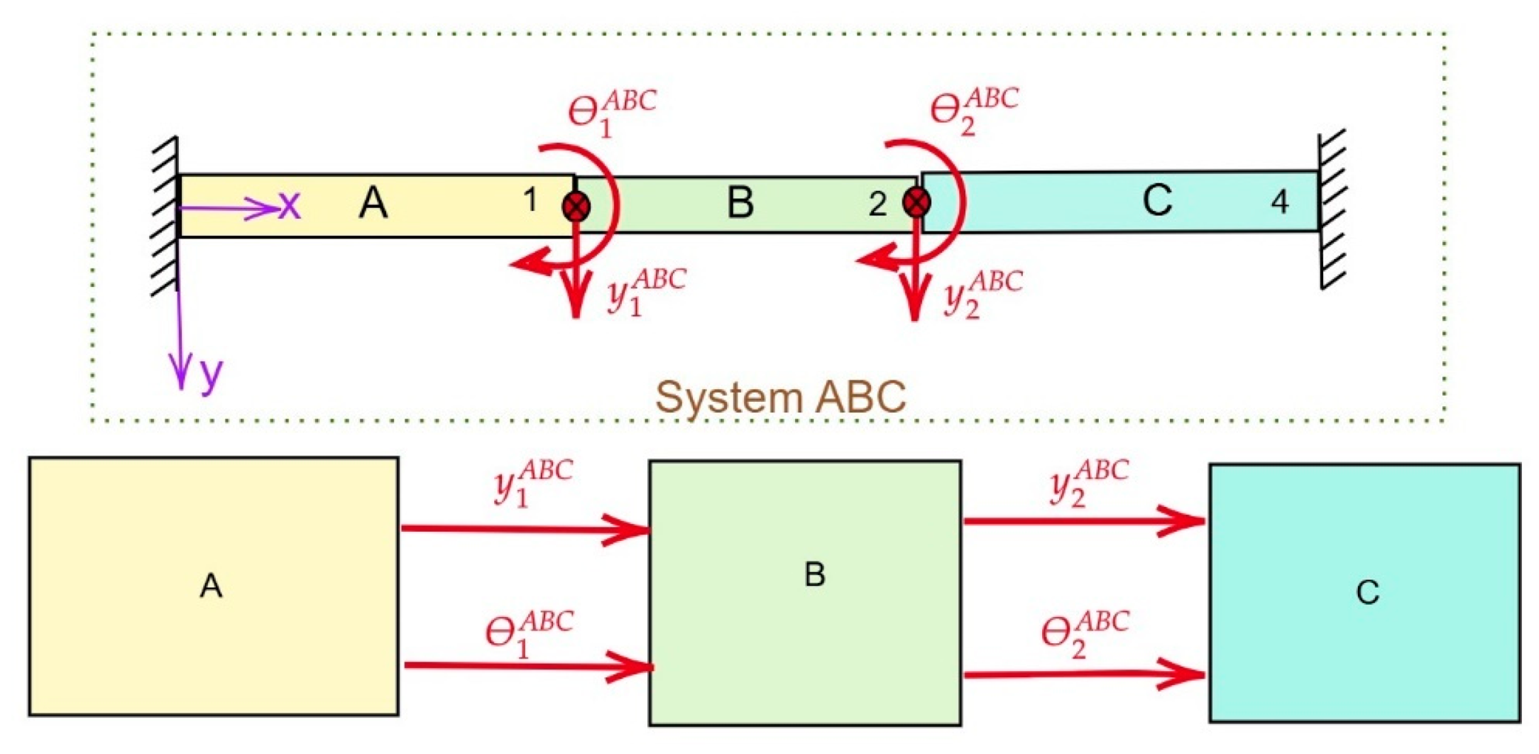
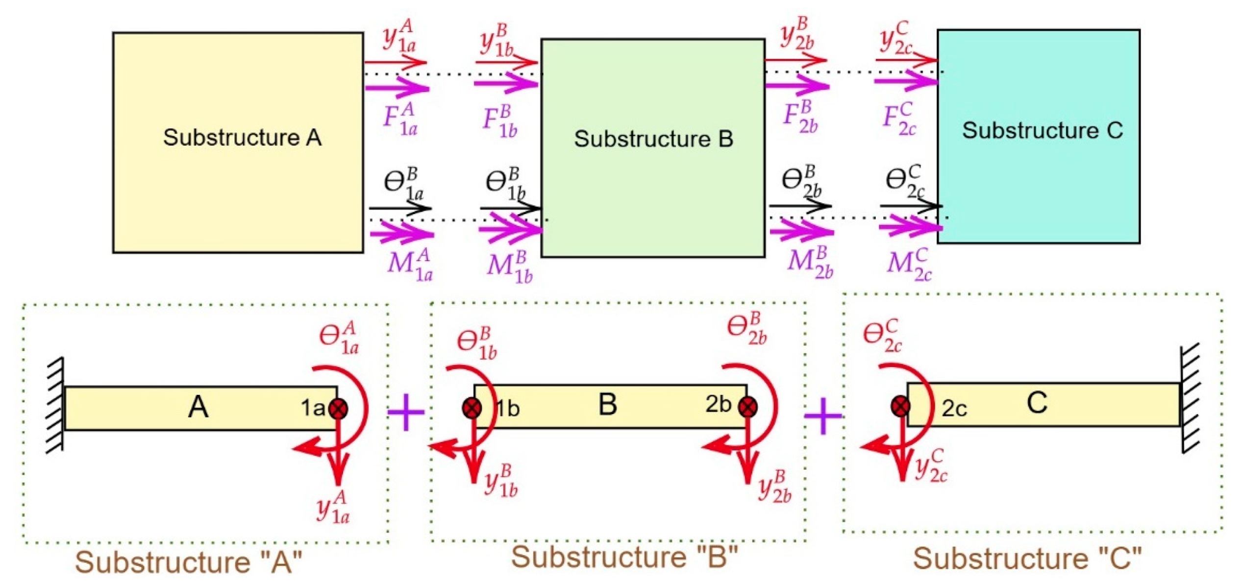
Figure 2 illustrates the assembly system (ABC), consisting of substructures A, B, and C, including their coordinates and DoFs at the connection points. The analysis focuses on the connection coordinates and corresponding DoFs, excluding internal coordinates.
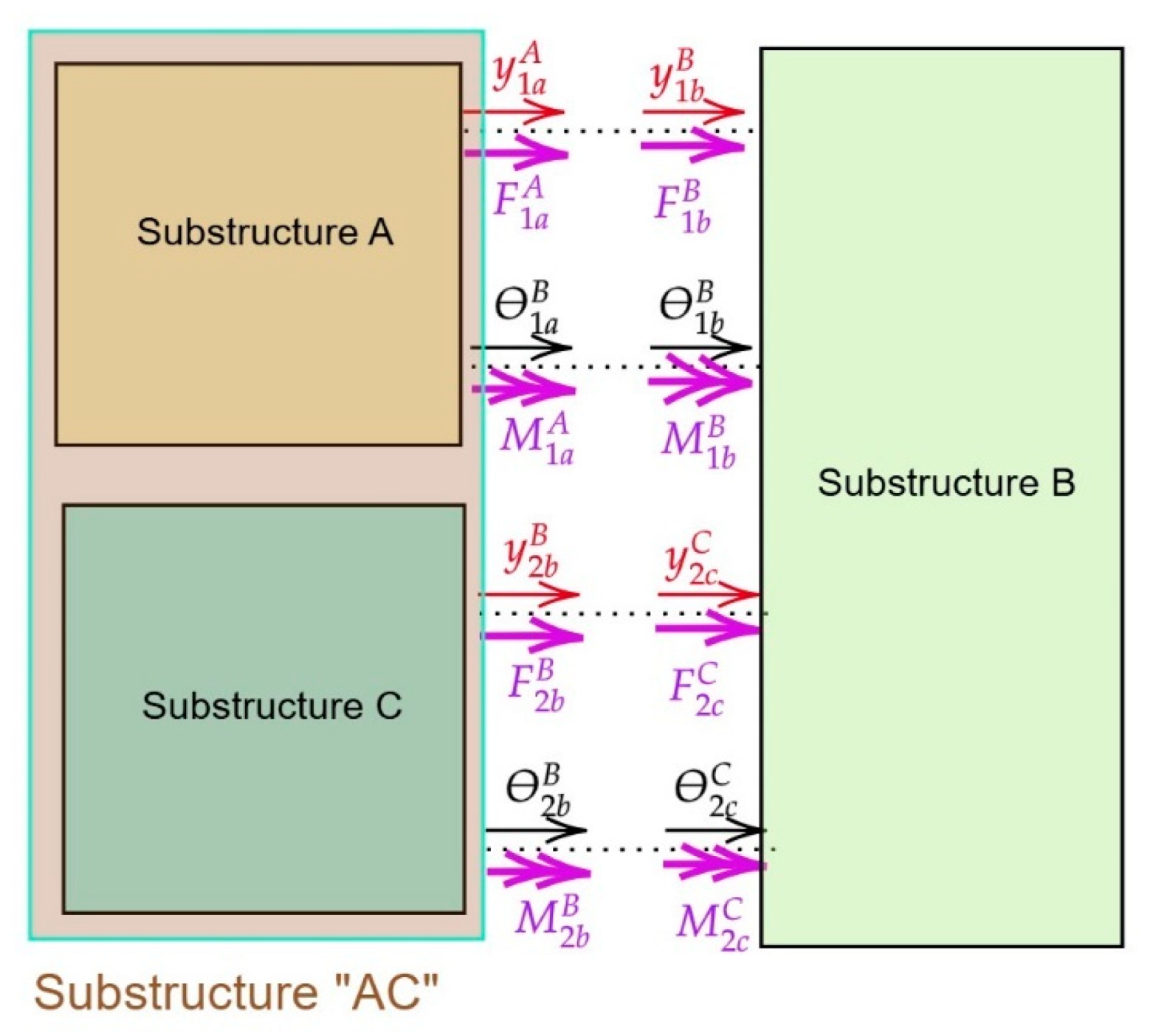
Due to system symmetry, substructures A and C are combined into a single substructure, AC. The receptance matrix for the combined substructure AC is diagonal, based on the receptance matrices of A and C. No cross-receptance components exist for AC, as there is no direct connection between A and C. Consequently, the problem is reduced to coupling two substructures, as depicted in Figure 3.
The receptance matrix for the combined subsystem AC is expressed as follows:
H A C 4 × 4 = H A 2 × 2 0 2 × 2 0 2 × 2 H C 2 × 2
The receptance coupling for the assembly of two substructures, as presented in Equation (1), simplifies in this case by omitting the internal body coordinates, resulting in Equation (8). In this configuration, substructure AC is coupled with substructure B at four connection points, in contrast to the two connection points used in the three-substructure case, to provide the receptance matrices for the assembly system ABC:
H c c A B C = H c c A C H c c A C H c c A C + H c c B 1 H c c A C

3.1.2. Validation of RCFBS Using Numerical FEA

The receptance matrix determined using the FBS method is validated through numerical FEA. The validation process involves comparing the dynamic response predictions based on the receptance matrix of subsystems A, B, and C using the RCFBS approach with the results obtained from the FEA [29]. In this section, the stiffness and mass matrices for each subsystem are derived. For subsystem A with 2 DoFs, the stiffness matrix [ K B ]   and mass matrix [ M B ]   are calculated as follows:
[ K A ] = E I A L A 3 12 6 L A 6 L A 4 L A 2 , [ M A ] = m A 420 156 22 L A 22 L A 4 L A 2 .
Similarly, for subsystem B with 4 DoFs, the stiffness [ K B ]   and mass matrix [ M B ]   are derived from the following:
[ K B ] = E I B L B 3 12 6 L B 12 6 L B 6 L B 4 L B 2 6 L B 2 L B 2 12 6 L B 12 6 L B 6 L B 2 L B 2 6 L B 4 L B 2 , [ M B ] = m B 420 156 22 L B 54 13 L B 22 L B 4 L B 2 13 L B 3 L B 2 54 13 L B 156 22 L B 13 L B 3 L B 2 22 L B 4 L B 2
For subsystem C, which also has 2 DoFs, the stiffness matrix [ K c ]   and mass matrix [ M c ]   a r e   c o m p u t e d   a s   f o l l o w s :
[ K c ] = E I c L c 3 12 6 L c 6 L c 4 L c 2 , [ M c ] = m c 420 156 22 L c 22 L c 4 L c 2
Eventually, the receptance matrix of each subsystem is determined by the following:
[ H i ] = [ ω 2 [ M i ] + [ K i ] ] 1 .
where index i represents subsystems A, B, and C. The global receptance matrix for the entire system ABC is obtained by assembling the global mass and stiffness matrices:
[ K A B C ] = 12 ( E I B L B 3 + E I A L A 3 ) 6 ( E I B L B 2 + E I A L A 2 ) 12 E I B L B 3 6 E I B L B 2 6 ( E I B L B 2 + E I A L A 2 ) 4 ( E I B L B + E I A L A ) 6 E I B L B 2 2 E I B L B 12 E I B L B 3 6 E I B L B 2 12 ( E I B L B 3 + E I c L c 3 ) 6 E I B L B 2 + E I c L B 2 6 E I B L B 2 2 E I B L B 6 ( E I B L B 2 + E I c L c 2 ) 4 ( E I B L B + E I c L c ) , [ M A B C ] = 1 420 156 m B + m A 22 ( L B m B L A m A ) 54 13 L B 22 ( L B m B L A m A ) 4 m A L A 2 + m B L B 2 13 L B 3 L B 2 54 13 L B 156 + 156 22 L B + L c 13 L B 3 L B 2 22 L B + L c 4 L B 2 + L c 2
Accordingly, the linear equations of motion for the assembly system AB are expressed as follows:
y 1 A B C θ 1 A B C y 2 A B C θ 2 A B C = [ H A B C ] F y 1 A B C F θ 1 A B C F y 2 A B C F θ 2 A B C .
Finally, the receptance matrix [ H A B C ] for the entire system ABC, using the direct method, is given by the following:
[ H A B C ] = H y 1 y 1 A B C H y 1 θ 1 A B C H y 1 y 2 A B C H y 1 θ 2 A B C H θ 1 y 1 A B C H θ 1 θ 1 A B C H θ 1 y 2 A B C H θ 1 θ 2 A B C H y 2 y 1 A B C H y 2 θ 1 A B C H y 2 y 2 A B C H y 2 θ 2 A B C H θ 2 y 1 A B C H θ 2 θ 1 A B C H θ 2 y 2 A B C H θ 2 θ 2 A B C = [ ω 2 [ M A B C ] + [ K A B C ] ] 1
This matrix encompasses both direct and cross-receptance components, which relate translational and rotational displacements to the applied forces and moments at various nodes. For instance, in the first column of the matrix, H y 1 y 1 A B C represents the translational displacement at node 1 due to a force applied at the same node, while H θ 1 y 1 A B C indicates the rotational displacement at node 1 caused by the force applied in the same node. Similarly, H y 2 y 1 A B C and H θ 2 y 1 A B C correspond to the translational and rotational displacements at node 2 resulting from a force applied at node 1. Although the frequency-based substructuring (FBS) method employs consistent generalized coordinates and degrees of freedom across substructures, further discretization through finite element analysis (FEA) can enhance the accuracy of the results.

3.1.3. Validation of RCFBS Using Modal Method

To determine the receptance matrix components for system ABC, modeled as a flexural beam with fixed-free boundary conditions, the mode shapes Y n x are derived from the Euler–Bernoulli beam theory. The mode shapes are given by the following [1]:
Y n x = cos h ( λ n x ) cos ( λ n x ) + cos h ( λ n L ) cos ( λ n L ) sin h ( λ n L ) sin ( λ n L ) ( sinh ( λ n x ) sin ( λ n x ) ) . θ n x = d Y n d x = λ n { sin h ( λ n x ) + sin ( λ n x ) + cos h ( λ n L ) cos ( λ n L ) sin h ( λ n L ) sin ( λ n L ) ( cosh ( λ n x ) c o s ( λ n x ) ) .
where θ n x   is the rotational mode shape (slope) evaluated at position x, derived from Y n x   and λ n 4 = ω n 2 ρ A E I , representing the n-th eigenvalue associated with the natural frequencies ω n   and mode shapes of the beam. The natural frequencies are obtained by solving the transcendental characteristic equation:
cos h ( λ n L ) cos ( λ n L ) = 1
Solving this equation yields multiple solutions, with the first four modes given by the following:
λ 1 L = 4.73 , λ 2 L = 7.85 , λ 3 L = 10.99 , λ 4 L = 14.13
This equation yields multiple solutions, with the first four modes corresponding to the natural frequencies of 20.03 Hz, 55.18 Hz, 108.15 Hz, and 178.96 Hz. The receptance is calculated by summing the contributions from each mode, using the mode shapes and natural frequencies to determine the response at a given excitation frequency. Given the assumption of no internal points, the receptance matrix H i j ω , which relates the translational or rotational displacement at connection points 1 and 2 (as shown in Figure 2) to the applied force or moment, is computed by summing the contributions from each mode:
H i j ω = r = 1 ψ i r ( x i ) ψ j r ( x i ) m ω r 2 ω 2
where m is the mass per unit length, ω r is the natural frequency of the r-th mode, and ψ i r ( x i ) represents the mode shape at position x i for the frequency ω r . This receptance function, H i j ω , characterizes the translational or rotational receptance at point x i due to a force or moment applied at point x j . It encapsulates the cumulative effect of each mode, with mode shapes evaluated at x i , and is pivotal in understanding the system’s dynamic response to excitations. For example, by considering contributions from the first four modes, the receptance functions H 11 ω , H 14 ω , a n d   H 22 ω , which describe the translational displacement at node 1 due to an excitation force applied at the same node, the translational displacement at node 1 due to an excitation moment applied at node 2, and the rotational displacement at node 1 due to a couple excitation applied at the same node, respectively, can be expressed as in Equation (20):
H 11 ω = X 1 F 1 = 1 m Y 11 2 ( x 1 ) ω 1 2 ω 2 + Y 12 2 ( x 1 ) ω 2 2 ω 2 + Y 13 2 ( x 1 ) ω 3 2 ω 2 + Y 14 2 ( x 1 ) ω 4 2 ω 2 H 14 ω = X 1 M 2 = 1 m Y 11 ( x 1 )   θ 21 ( x 2 ) ω 1 2 ω 2 + Y 12 ( x 1 )   θ 22 ( x 2 ) ω 2 2 ω 2 + Y 13 ( x 1 )   θ 23 ( x 2 ) ω 3 2 ω 2 + Y 14 ( x 1 )   θ 24 ( x 2 ) ω 4 2 ω 2 H 22 ω =   θ 1 M 1 = 1 m   θ 11 2 ( x 1 ) ω 1 2 ω 2 +   θ 12 2 ( x 1 ) ω 2 2 ω 2 +   θ 13 2 ( x 1 ) ω 3 2 ω 2 +   θ 14 2 ( x 1 ) ω 4 2 ω 2
These components are integral to understanding the system’s dynamic response to various types of excitations.

3.1.4. Results: Comparison Between Receptance Coupling from Different Methods

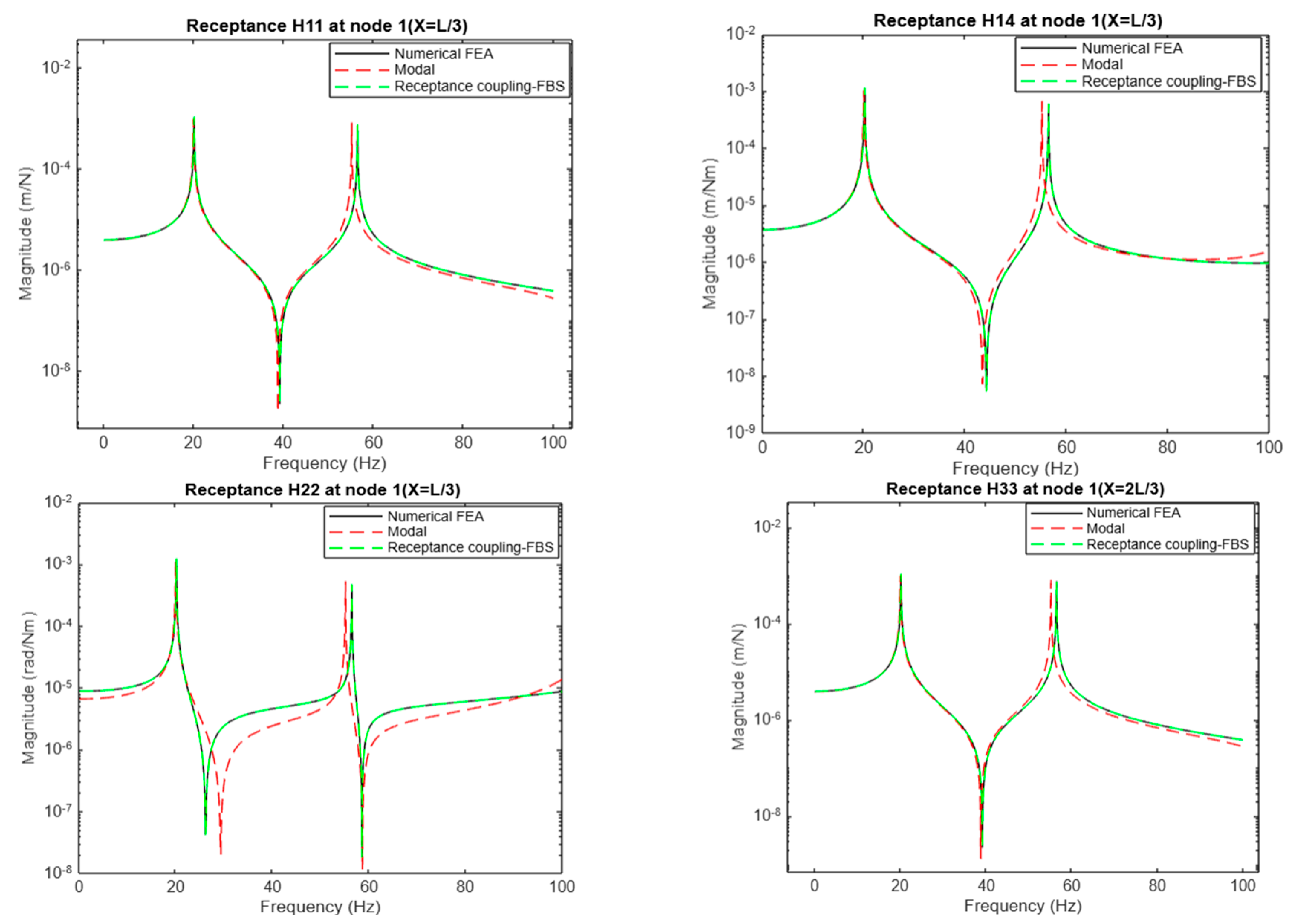
Figure 4 and Figure 5 illustrate the comparison of receptance coupling using frequency-based substructuring (RCFBS), the modal method, and numerical finite element analysis (FEA). In the frequency range of up to 100 Hz, which encompasses the first two dominant modes, all methods show a strong agreement in the resonance and anti-resonance peaks. However, at higher frequencies, particularly around 400 Hz, discrepancies arise. While FEA and RCFBS maintain consistency, the modal method deviates, with noticeable differences in the fourth mode compared to the third.
The material properties and structural parameters used for modeling are presented in Table 1.

3.1.5. Discrepancy Analysis

The discrepancies observed in the modal method can be attributed to several factors. The modal method relies on analytical solutions to derive the mode shapes and compute the receptance by summing the contributions from selected modes. This approach, however, involves mode truncation, which limits the representation of higher-frequency contributions and, particularly, impacts the rotational receptance due to the complexity of the interactions between the rotational displacement and force excitation. In contrast, both the FEA and frequency-based substructuring (FBS) methods discretize the structure into elements or substructures, using the stiffness and mass matrices to calculate receptance. This discrete representation maintains consistent degrees of freedom and captures the dynamics more accurately, especially at higher modes.
While all methods exhibit similar resonance trends up to 400 Hz, the modal method begins to show discrepancies at higher frequencies. Specifically, the modal method’s peak resonance and anti-resonance shift for the higher modes indicate a tendency to present softer behavior in high frequencies due to the incomplete stiffness contributions. This limitation is more pronounced for the rotational receptance compared to the translational receptance. The FBS method, by dividing complex structures into smaller substructures, captures the interactions of local dynamics and higher modes more precisely. Therefore, it provides more accurate predictions across a broad frequency range compared to the modal method, which may oversimplify high-frequency dynamics and localized effects.

3.1.6. Validation and Reliability

The frequency-based substructuring (FBS) method aligns more closely with the finite element method (FEM) results for higher modes, indicating its superior accuracy in representing a structure’s dynamic behavior, particularly where local effects and substructure interactions are significant. While the modal method effectively captures the primary modes, it often oversimplifies the response in higher modes, where detailed local effects and interface interactions become critical. FBS addresses these interactions by incorporating the dynamic stiffness and receptance matrices at interfaces, leading to results that more accurately reflect the FEM, a concept referred to as interface dynamics. This makes FBS particularly reliable for applications requiring precise predictions of higher modes, such as in noise, vibration, and harshness (NVH) or high-frequency vibration control studies in vehicle applications.
In the comparison of receptance components—H11, H14, H22, and H33—up to 100 Hz, all three methods show strong agreement. Notably, H22, which represents the rotational receptance at node 1 due to a couple excitation at the same node, exhibits the most significant error. Figure 4 and Figure 5 illustrate that the translational receptance components H11 and H33, due to symmetry, match exactly across methods. The modal method performs slightly better for these translational components, but it shows larger discrepancies for rotational receptance components H14 and H22, which involve complex interactions of the rotational displacement and moments.

3.2. Case Study 2: Coupling of Subsystems with Lumped Parameters

In the previous case, the receptance coupling method using frequency-based substructuring (RCFBS) is validated for a dynamic structure with continuous characteristics. In this case study, the same approach is applied to a system with lumped specifications.

3.2.1. RCFBS Method and Governing Equations

This example provides fundamental details for determining the receptance components of a system denoted as AB, which consists of four generalized coordinates, each with one translational degree of freedom (DoF), resulting in a total of four DoFs. The system is decomposed into two subsystems, A and B, each having three generalized coordinates with one translational DoF. Figure 6 illustrates the original assembly system AB and its decomposition into independent subsystems A and B.
During the partitioning, mass m25 is divided into masses m2 and m5, while mass m36 is split into masses m3 and m6. Each partitioned mass is assigned to a different subsystem, with one part belonging to subsystem A and the other to subsystem B. The connection between the subsystems is established through two rigid connection points along the partition line. Both subsystems consist of multiple lumped masses, springs, and dampers. Unlike the previous case, the inclusion of internal DoFs within these subsystems adds complexity, which is effectively managed using the RCFBS method. Figure 6a shows the assembly system AB, Figure 6b presents the generalized coordinates at internal and connection points, and Figure 6c illustrates the substructuring scheme for decomposing system AB into subsystems A and B.
The receptance components are first calculated using the RCFBS method. These findings are subsequently validated by comparing them with the direct method and the modal method. The derivation of the receptance elements begins by assigning generalized coordinates and relevant DoFs based on boundary conditions, using the receptance coupling method based on FBS. The RCFBS method involves solving the equations of motion by maintaining force equilibrium and ensuring compatibility at the points of connection. Once these equations are solved, the receptance matrix HAB is obtained. Additionally, the receptance matrix components for the assembly system AB are presented in terms of the substructures’ receptance using the generalized receptance coupling frequency-based substructuring (GRCFBS) formula, which is more effective than classical RCFBS formulations for complex systems. The validation of this case study is further supported by a comparison with the direct and modal methods.
The equations of motions for substructure A and B, based on the generalized coordinates shown in Figure 6b, are expressed as follows:
H u 1 u 1 A H u 1 u c 1 A H u 1 u c 2 A H u c 1 u 1 A H u c 1 u c 1 A H u c 1 u c 2 A H u c 2 u 1 A H u c 2 u c 1 A H u c 2 u c 2 A F u 1 A F u c 1 A F u c 2 A = u 1 A u u c 1 A u u c 2 A ,   H u 4 u 4 B H u 4 u c 1 B H u 4 u c 2 B H u c 1 u 4 B H u c 1 u c 1 B H u c 1 u c 2 B H u c 2 u 4 B H u c 2 u c 1 B H u c 2 u c 2 B F u 4 B F u c 1 B F u c 2 B = u 4 B u u c 1 B u u c 2 B .
The boundary conditions, including equilibrium and compatibility, are given by the following:
F u c 1 e x t = F u c 1 A + F u c 1 B F u c 1 A = K 1 ( u u c 1 A u u c 1 B ) ;   F u c 2 e x t = F u c 2 A + F u c 2 B F u c 2 A = K 2 ( u u c 2 A u u c 2 B ) ,
where K 1 and K 2 represent the dynamic stiffness at the connection points.
To determine the direct receptance H u 1 u 1 A B , which is the displacement of system AB at coordinate u 1 A B due to an excitation applied at the same point ( H u 1 u 1 A B = u 1 A B F u 1 A B ), we start by determining u 1 A B based on the excitation force F u 1 A B . The equations of motion for assembly AB are given by the following:
H u 1 u 1 A B H u 1 u 2 A B H u 1 u 3 A B H u 1 u 4 A B H u 2 u 1 A B H u 2 u 2 A B H u 2 u 3 A B H u 2 u 4 A B H u 3 u 1 A B H u 3 u 2 A B H u 3 u 3 A B H u 3 u 4 A B H u 4 u 1 A B H u 4 u 2 A B H u 4 u 3 A B H u 4 u 4 A B F u 1 A B F u 2 A B F u 3 A B F u 4 A B = u 1 A B u 2 A B u 3 A B u 4 A B ;
Assuming that external excitation is applied only at the coordinate of measurement u1 and the connections are rigid, the boundary conditions in Equation (22) are simplified to the following:
F u c 1 A + F u c 1 B = 0 u u c 1 A u u c 1 B = 0 ;       F u c 2 A + F u c 2 B = 0 u u c 2 A u u c 2 B = 0
By substituting Equation (21) into the simplified boundary conditions in Equation (24), we obtain the following:
u u c 1 A = u u c 1 B y i e l d s H u c 1 u 1 A F u 1 A + H u c 1 u c 1 A F u c 1 A + H u c 1 u c 2 A F u c 2 A = H u c 1 u 4 B F u 4 B + H u c 1 u c 1 B F u c 1 B + H u c 1 u c 2 B F u c 2 B u u c 2 A = u u c 2 B = 0 y i e l d s H u c 2 u 1 A F u 1 A + H u c 2 u c 1 A F u c 1 A + H u c 2 u c 2 A F u c 2 A = H u c 2 u 4 B F u 4 B + H u c 2 u c 1 B F u c 1 B + H u c 2 u c 2 B F u c 2 B
Assuming that the only excitation applied is F u 1 A B , the displacements at the coordinates of interest (u1, u2, u3, and u4) due to this excitation determine the first row of the assembly AB receptance matrix: H u 1 u 1 A B ,   H u 2 u 1 A B , H u 3 u 1 A B , and H u 4 u 1 A B . No excitation is applied at the rest of the points, so F u 2 A B = F u 3 A B = F u 4 A B = 0 . From Equations (24) and (25), we can write the following:
H u c 1 u 1 A F u 1 A = ( H u c 1 u c 1 A + H u c 1 u c 1 B ) F u c 1 A + H u c 1 u c 2 A + H u c 1 u c 2 B F u c 2 A H u c 2 u 1 A F u 1 A = ( H u c 2 u c 1 A + H u c 2 u c 1 B ) F u c 1 A + ( H u c 2 u c 2 A + H u c 2 u c 2 B ) F u c 2 A
Solving these equations to express F u c 1 A and F u c 2 A as functions of the receptance elements and F u 1 A leads to:
F u c 1 A = S 2 S 0 F u 1 A ,       F u c 2 A = S 1 S 0 F u 1 A where : S 0 = H u c 1 u c 2 A + H u c 1 u c 2 B 2 ( H u c 1 u c 1 A + H u c 1 u c 1 B ) ( H u c 2 u c 2 A + H u c 2 u c 2 B ) S 1 = H u c 1 u 1 A H u c 2 u c 1 A + H u c 2 u c 1 B H u c 2 u 1 A ( H u c 1 u c 1 A + H u c 1 u c 1 B ) S 2 = S 0 H u c 1 u 1 A + S 1 H u c 1 u c 2 A + H u c 1 u c 2 B H u c 1 u c 1 A + H u c 1 u c 1 B
Now, considering the continuity principles u 1 A B = u 1 A and F u 1 A B = F u 1 A , by substituting F u c 1 A and F u c 2 A from Equation (27) into Equation (21), the receptance element H u 1 u 1 A B can be obtained as follows:
H u 1 u 1 A B = u 1 A B F u 1 A B = H u 1 u 1 A F u 1 A + H u 1 u c 1 A F u c 1 A + H u 1 u c 2 A F u c 2 A F u 1 A = H u 1 u 1 A H u 1 u c 1 A S 2 + H u 1 u c 2 A S 1 S 0
Similarly, H u 2 u 1 A B is determined using the continuity condition u 2 A B = u u c 1 B   = u u c 1 A . The receptance elements H u 2 u 1 A B , H u 3 u 1 A B , and H u 4 u 1 A B represent the responses of the assembly AB, corresponding to the displacements at coordinates u2, u3, and u4 belonging to lumped mass m25, m36, and m4, respectively, due to generating an excitation force at coordinate u1 (lumped mass m1), as presented in Equation (29):
H u 2 u 1 A B = u 2 A B F u 1 A B = u u c 1 B F u 1 A = H u c 1 u c 1 B F u c 1 B + H u c 1 u c 2 B F u c 2 B F u 1 A = H u c 1 u c 1 B F u c 1 A + H u c 1 u c 2 B F u c 2 A F u 1 A = H u c 1 u c 1 B S 2 + H u c 1 u c 2 B S 1 S 0 H u 3 u 1 A B = u 3 A B F u 1 A B = u u c 2 B F u 1 A = H u c 2 u c 1 B F u c 1 B + H u c 2 u c 2 B F u c 2 B F u 1 A = H u c 2 u c 1 B F u c 1 A + H u c 2 u c 2 B F u c 2 A F u 1 A = H u c 2 u c 1 B S 2 + H u c 2 u c 2 B S 1 S 0 H u 4 u 1 A B = u 4 A B F u 1 A B = u u 4 B F u 1 A = H u 4 u c 1 B F u c 1 B + H u 4 u c 2 B F u c 2 B F u 1 A = H u 4 u c 1 B F u c 1 A + H u 4 u c 2 B F u c 2 A F u 1 A = H u 4 u c 1 B S 2 + H u 4 u c 2 B S 1 S 0
It should be noted that, due to the reciprocity principle, H u 1 u 2 A B = H u 2 u 1 A B , H u 1 u 3 A B = H u 3 u 1 A B , H u 1 u 4 A B = H u 4 u 1 A B . To determine H u 2 u 4 A B ,   H u 3 u 4 A B ,   a n d   H u 4 u 4 A B , the assumption is modified so that the only excitation force applied to the system AB is F u 4 A B , with F u 2 A B = F u 3 A B = F u 1 A B = 0 . The goal is to determine the displacement at the coordinates of interest (u2, u3, and u4), which corresponds to the elements in the fourth column of the assembly AB receptance matrix. From Equation (21) and considering the above assumptions, the following can be expressed:
H u c 1 u 4 B F u 4 B = ( H u c 1 u c 1 A + H u c 1 u c 1 B ) F u c 1 A + H u c 1 u c 2 A + H u c 1 u c 2 B F u c 2 A H u c 2 u 4 A F u 4 B = ( H u c 2 u c 1 A + H u c 2 u c 1 B ) F u c 1 A + ( H u c 2 u c 2 A + H u c 2 u c 2 B ) F u c 2 A
Then, by solving Equation (30), F u c 1 A and F u c 2 A can be determined as functions of the receptance elements and F u 1 A as follows:
F u c 2 A = S 3 S 0 F u 4 B ,       F u c 1 A = S 4 S 0 F u 4 B where : S 3 = H u c 2 u 4 B ( H u c 1 u c 1 A + H u c 1 u c 1 B ) H u c 1 u 4 B H u c 2 u c 1 A + H u c 2 u c 1 B S 4 = S 0 H u c 1 u 4 B S 3 H u c 1 u c 2 A + H u c 1 u c 2 B H u c 1 u c 1 A + H u c 1 u c 1 B
Based on the continuity conditions u 4 A B = u 4 B and F u 4 A B = F u 4 B , u 2 A B = u u c 1 B , u 3 A B = u u c 2 B , and substituting F u c 1 A and F u c 2 A from Equation (31) into Equation (21), H u 4 u 4 A B can be obtained based on the definition of the receptance function:
H u 2 u 4 A B = u 2 A B F u 4 A B = H u c 1 u 4 B F u 4 B + H u c 1 u c 1 B F u c 1 B + H u c 1 u c 2 B F u c 2 B F u 4 B = H u c 1 u 4 B H u c 1 u c 1 B S 4 + H u c 1 u c 2 B S 3 S 0 H u 3 u 4 A B = u 3 A B F u 4 A B = u u c 2 B F u 4 B = H u c 2 u 4 B F u 4 B + H u c 2 u c 1 B F u c 1 B + H u c 2 u c 2 B F u c 2 B F u 4 B = H u c 2 u 4 B H u c 2 u c 1 B S 4 + H u c 2 u c 2 B S 3 S 0 H u 4 u 4 A B = u 4 A B F u 4 A B = u u 4 B F u 4 B = H u 4 u 4 B F u 4 B + H u 4 u c 1 B F u c 1 B + H u 4 u c 2 B F u c 2 B F u 4 B = H u 4 u 4 B H u 4 u c 1 B S 4 + H u 4 u c 2 B S 3 S 0
where H u 2 u 4 A B ,   H u 3 u 4 A B ,     a n d   H u 4 u 4 A B provide the receptance functions of assembly AB based on the displacements at coordinates u2, u3, and u4 corresponding with lumped mass m25, m36, and m4 due to applying an excitation force at coordinate u4 (lumped mass m4), respectively. This technique is particularly useful as it allows the indirect determination of the receptance at the connection points, which are often challenging to measure or simulate numerically. The chain rule and symmetry properties of the receptance elements help in deriving the coupling receptance components as follows:
H u 2 u 2 A B = H u 2 u 1 A B ( H u 1 u 1 A B ) 1 H u 1 u 2 A B = H u 2 u 1 A B ( H u 1 u 1 A B ) 1 H u 2 u 1 A B H u 3 u 3 A B = H u 3 u 1 A B ( H u 1 u 1 A B ) 1 H u 1 u 3 A B = H u 3 u 1 A B ( H u 1 u 1 A B ) 1 H u 3 u 1 A B H u 3 u 4 A B = H u 3 u 1 A B ( H u 4 u 1 A B ) 1 H u 4 u 4 A B
The advantage of this coupling method is its ability to significantly reduce the number of measurements and calculations required to develop effective vibrational models. Due to the reciprocity principle and the application of the chain rule, the full system receptance matrix, which consists of 16 elements, can be determined by determining the elements of one column or row from the substructures when they are disassembled. It is important to note that, when any receptance element like H u 1 u 1 A B approaches infinity, it indicates resonance in the assembled system and provides the natural frequency of the entire system. Consequently, the natural frequencies ω 1 2 , ω 2 2 , ω 3 2 , a n d   ω 4 2 can be directly determined from the frequency equation by setting S 0 = 0 . Additionally, the fundamental development using the RCFBS method can be expressed in the generalized form of Equation (1), which presents the coupling of two substructures under the discussed assumptions.
H u 1 u 1 A B H u 1 u 2 A B H u 1 u 3 A B H u 1 u 4 A B H u 2 u 1 A B H u 2 u 2 A B H u 2 u 3 A B H u 2 u 4 A B H u 3 u 1 A B H u 3 u 2 A B H u 3 u 3 A B H u 3 u 4 A B H u 4 u 1 A B H u 4 u 2 A B H u 4 u 3 A B H u 4 u 4 A B = H u 1 u 1 A H u 1 u c 1 A H u 1 u c 2 A 0 H u c 1 u 1 A H u c 1 u c 1 A H u c 1 u c 2 A 0 H u c 2 u 1 A H u c 2 u c 1 A H u c 2 u c 2 A 0 0 0 0 H u 4 u 4 B H u 1 u c 1 A H u 1 u c 2 A H u c 1 u c 1 A H u c 1 u c 2 A H u c 2 u c 1 A H u c 2 u c 2 A H u 4 u c 1 B H u 4 u c 2 B H u c 1 u c 1 A H u c 1 u c 2 A H u c 2 u c 1 A H u c 2 u c 2 A + H u c 1 u c 1 B H u c 1 u c 2 B H u c 2 u c 1 B H u c 2 u c 2 B 1 H u 1 u c 1 A H u 1 u c 2 A H u c 1 u c 1 A H u c 1 u c 2 A H u c 2 u c 1 A H u c 2 u c 2 A H u 4 u c 1 B H u 4 u c 2 B T
To determine the receptance components of subsystems A and B in their disassembled conditions, it is essential to evaluate them as independent substructures separately. As illustrated in Figure 6b, when system AB is partitioned into subsystems A and B, there are two generalized coordinates, uc1 and uc2, at the interface or connection area. Equation (34) demonstrates that the receptance of system AB depends on the receptance matrices of subsystems A and B, which are determined through either measurement or numerical analysis. Depending on the complexity and availability of the data, the frequency response function (FRF) matrix of the substructures can be obtained via direct measurement, or analytical or numerical methods. In this case, an analytical method can be employed to derive the receptance (FRF) matrix components at the points of interest.
  • Equations of motion for subsystem A:
For subsystem A, the generalized coordinate of interest consists of uc1 and uc2 at the connection points and u1 as an internal coordinate. The equations of motion in the time domain are formulated as follows:
M A u 1 ¨ u ¨ c 1 u ¨ c 2 + C A u ˙ 1 u ˙ c 1 u ˙ c 2 + K A u 1 u c 1 u c 2 = f t , where : M A = m 11 A 0 0 0 m 22 A 0 0 0 m 33 A , C A = c 11 A c 12 A c 13 A c 21 A c 22 A c 23 A c 31 A c 32 A c 33 A ,   K A = k 11 A k 12 A k 13 A k 21 A k 22 A k 23 A k 31 A k 32 A k 33 A
By transferring these equations of motion from the time domain to the frequency domain, the receptance matrix can be determined as follows:
H A ω F u 1 A F u c 1 A F u c 2 A = u 1 A u u c 1 A u u c 2 A where : H A ω = ( K A + j ω C A ω 2 M A ) 1 = H u 1 u 1 A H u 1 u c 1 A H u 1 u c 2 A H u c 1 u 1 A H u c 1 u c 1 A H u c 1 u c 2 A H u c 2 u 1 A H u c 2 u c 1 A H u c 2 u c 2 A
  • Equations of motion for subsystem B:
Similarly, for subsystem B, the generalized coordinates of interest are uc1 and uc2 at the connection points and u4 as an internal coordinate. The equations of motion are as follows:
M B u 4 ¨ u ¨ c 1 u ¨ c 2 + C B u ˙ 4 u ˙ c 1 u ˙ c 2 + K B u 4 u c 1 u c 2 = f t where : M B = m 11 B 0 0 0 m 22 B 0 0 0 m 33 B , C B = c 11 B c 12 B c 13 B c 21 B c 22 B c 23 B c 31 B c 32 B c 33 B ,   K B = k 11 B k 12 B k 13 B k 21 B k 22 B k 23 B k 31 B k 32 B k 33 B
The receptance matrix for subsystem B is then determined as follows:
H B ω F u 4 B F u c 1 B F u c 2 B = u 4 B u u c 1 B u u c 2 B where : H B ω = ( K B + j ω C B ω 2 M B ) 1 = H u 4 u 4 B H u 4 u c 1 B H u 4 u c 2 B H u c 1 u 4 B H u c 1 u c 1 B H u c 1 u c 2 B H u c 2 u 4 B H u c 2 u c 1 B H u c 2 u c 2 B
where the terms for the stiffness, damping, and mass matrices are as follows:
For subsystem A:
m 11 A = m 1 ,   m 22 A = m 2 ,   m 33 A = m 3 ,   C 11 A = ( C 1 + C 2 + C 3 ) ,   C 12 A = C 21 A = C 2 ,   C 13 A = C 31 A = C 3 ,   C 22 A = C 2 ,   C 23 A = C 32 A = 0 ,   C 33 A = C 3 ,   k 11 A = ( k 1 + k 2 + k 3 ) ,   k 12 A = k 21 A = k 2 ,   k 13 A = k 31 A = k 3 ,   k 22 A = k 2 ,   k 23 A = k 32 A = 0 ,   k 33 A = k 3  
For subsystem B:
m 11 B = m 4 ,   m 22 B = m 5 ,   m 33 B = m 6 ,   C 11 B = ( C 4 + C 5 + C 6 ) ,   C 12 B = C 21 B = C 5 ,   C 13 B = C 31 B = C 6 ,   C 22 B = C 5 ,   C 23 B = C 32 B = 0 ,   C 33 B = C 6 ,   k 11 B = ( k 4 + k 5 + k 6 ) ,   k 12 B = k 21 B = k 5 ,   k 13 B = k 31 B = k 6 ,   k 22 B = k 5 ,   k 23 B = k 32 B = 0 ,   k 33 B = k 6  
Using Equation (34), the receptance matrix and its components for the assembly AB can be calculated based on the decoupled receptance components of subsystems A and B, as determined from Equations (36) and (38). As depicted in Figure 6, the employment of the substructuring scheme using RCFBS reduces the original 4-DOF system to a simplified form, consisting of two simpler and more manageable substructures, A and B, each with 3 DOFs, connected through the generalized coordinates uc1 and uc2. The lumped parameters for the 4-DOF system in this case study are provided in Table 2.

3.2.2. Validation Approach Using Direct Method

For the complete system AB, which consists of four generalized coordinates as illustrated in Figure 6a, the equations of motion are expressed as follows:
M A B u 1 ¨ u ¨ 2 u ¨ 3 u ¨ 4 + C A B u ˙ 1 u ˙ 2 u ˙ 3 u ˙ 4 + K A B u 1 u 2 u 3 u 4 = f t
The mass, damping, and stiffness matrices are defined as follows:
M A B = m 11 A B 0 0 0 0 m 22 A B 0 0 0 0 m 33 A B 0 0 0 0 m 44 A B , C A B = c 11 A B c 12 A B c 13 A B c 14 A B c 21 A B c 22 A B c 23 A B c 24 A B c 31 A B c 32 A B c 33 A B c 34 A B c 41 A B c 42 A B c 43 A B c 44 A B , K A B = k 11 A B k 12 A B k 13 A B k 14 A B k 21 A B k 22 A B k 23 A B k 24 A B k 31 A B k 32 A B k 33 A B k 34 A B k 41 A B k 42 A B k 43 A B k 44 A B
By transforming the equations of motion from the time domain to the frequency domain, we obtain the following:
H A B ω F u 1 A B F u 2 A B F u 3 A B F u 4 A B = u 1 A B u 2 A B u 3 A B u 4 A B , where : H A B ω = ( K A B + j ω C A B ω 2 M A B ) 1 = H u 1 u 1 A B H u 1 u 2 A B H u 1 u 3 A B H u 1 u 4 A B H u 2 u 1 A B H u 2 u 2 A B H u 2 u 3 A B H u 2 u 4 A B H u 3 u 1 A B H u 3 u 2 A B H u 3 u 3 A B H u 3 u 4 A B H u 4 u 1 A B H u 4 u 2 A B H u 4 u 3 A B H u 4 u 4 A B
where the terms for the stiffness, damping, and mass matrices for subsystem AB are as follows:
m 11 A B = m 1 ,   m 22 A B = m 25 = m 2 + m 5 ,   m 33 A B = m 36 = m 3 + m 6 , C 11 A B = ( C 1 + C 2 + C 3 ) ,   C 12 A B = C 21 A B = C 2   ,   C 13 A B = C 31 A B = C 3 ,     C 14 A B = C 41 A B = 0 , C 22 A B = C 2 + C 5 ,   C 23 A B = C 32 A B = 0 , ,   C 24 A B = C 42 A B = C 5   , C 33 A B = C 3 + C 6   , C 33 A B = C 3 + C 6   ,   C 34 A B = C 43 A B = C 6 , C 44 A B = ( C 4 + C 5 + C 6 ) , k 11 A B = ( k 1 + k 2 + k 3 ) ,   k 12 A B = k 21 A B = k 2   ,   k 13 A B = k 31 A B = k 3 ,     k 14 A B = k 41 A B = 0 , k 22 A B = k 2 + k 5 ,   k 23 A B = k 32 A B = 0 ,   k 24 A B = k 42 A B = k 5   , k 33 A B = k 5   , k 33 A B = k 3 + k 6   ,   k 34 A B = k 43 A B = k 6 , k 44 A B = ( k 4 + k 5 + k 6 ) .

3.2.3. Validation Approach Using the Modal Method

As previously discussed in the earlier case study, the modal approach offers a systematic way to validate the dynamic behavior of the system by analyzing its natural frequencies and mode shapes. For the second case study, this approach is employed to ensure consistency and accuracy across different validation methods. To apply the modal method to the entire system AB, the natural frequencies and mode shapes can be determined by solving the eigenvalue problem. By obtaining these natural frequencies and mode shapes, it becomes possible to compute the components of the receptance matrices based on Equation (4). This approach provides a comprehensive validation framework, ensuring that the receptance matrix components derived through the modal method align with those obtained from other methods, thereby reinforcing the robustness of the results.

3.2.4. Results: Comparison of Receptance Components Across Different Methods

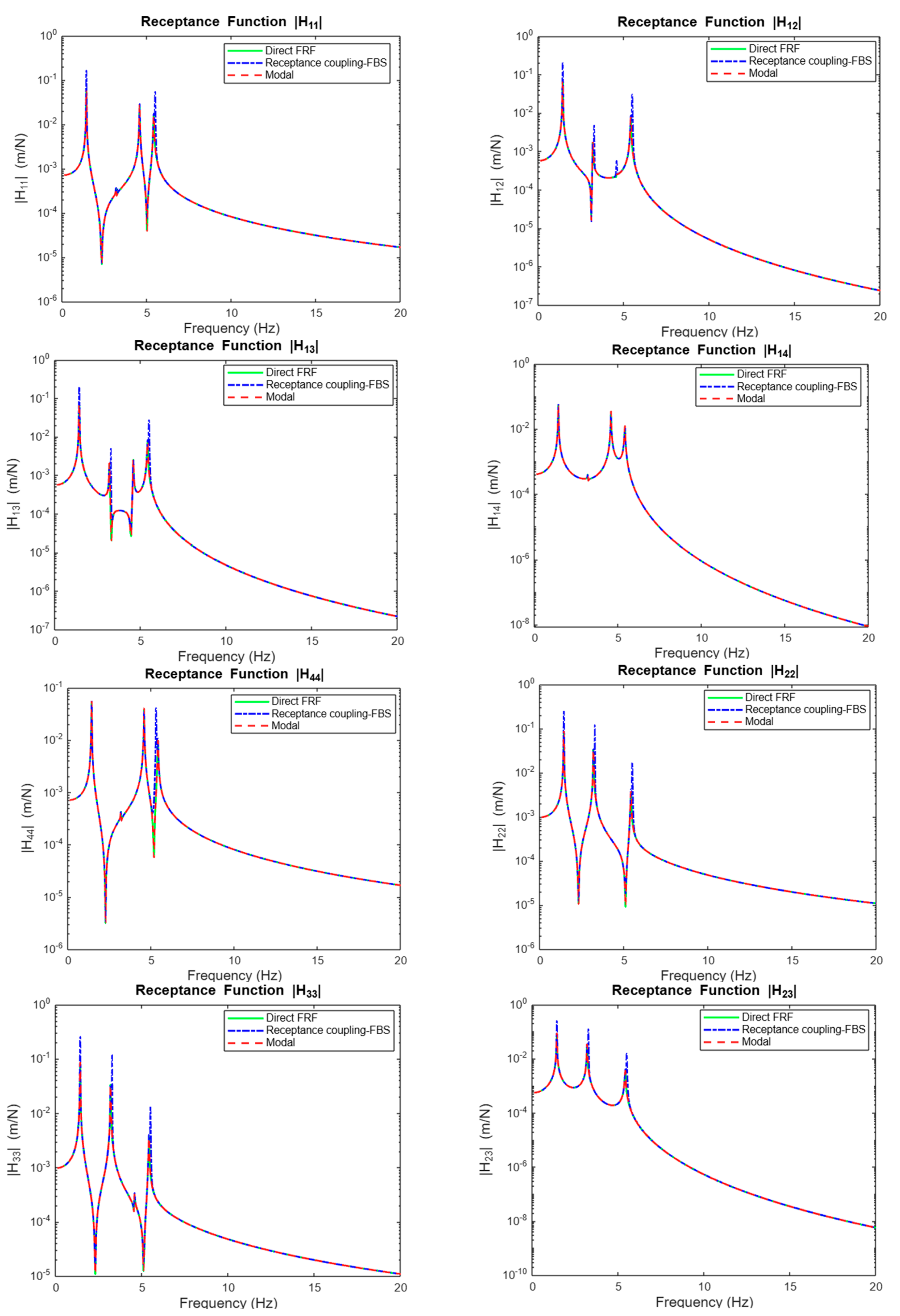
Following the methodology outlined in the previous case study, the most straightforward approach for validating the results obtained from the receptance coupling and frequency-based substructuring (RCFBS) method is through a direct comparison with results from other established methods. In this study, the direct method, representative of an exact solution, and the modal method were employed for this purpose. A comparative simulation was conducted in MATLAB (2023b) using the theoretical approaches and parameters discussed earlier. The results, as shown in Figure 7, demonstrate a strong correlation between the RCFBS method and the other methods, particularly in terms of resonance peaks and natural frequencies. Specifically, the natural frequencies obtained via the RCFBS method for the four modes are 1.416, 3.25, 4.64, and 5.48 Hz. The corresponding frequencies from the direct and modal methods are 1.410, 3.177, 4.565, and 5.396 Hz, respectively. The differences are minimal, with deviations of 0.4%, 2%, 1.7%, and 1.5%, respectively. This slight increase in natural frequencies observed in the RCFBS method suggests a higher system stiffness, which is also reflected in the increased peak magnitudes. Beyond resonance peaks, there is a notable consistency between the methods in the anti-resonance regions as well, indicating that the dynamic response characteristics are reliably captured across the different approaches. In the context of this lumped-parameter system, the modal method does not suffer from mode truncation, unlike in continuous or distributed-parameter systems discussed in the previous case study. As a result, all methods are based on the same degrees of freedom (DoFs), leading to a more precise alignment in the results.
As anticipated, all receptance components exhibit similar resonance peaks, which validates the accuracy of the results, given that natural frequencies are intrinsic properties of the system and are independent of the excitation point. Additionally, there is a strong agreement between both the cross-receptance components (H12, H13, H14, and H23) and the direct receptance components (H11, H22, H33, and H44). Synthesizing the findings from the two different case studies, it is evident that the RCFBS method provides a reliable and effective solution for the reduced-order modeling of dynamic structures, showing comparable results to other methods. Importantly, RCFBS demonstrates superiority over the modal method in distributed-parameter systems due to its avoidance of mode truncation limitations.
It is worth noting that the partitioning scheme employed in this study was based on trimming two masses associated with generalized coordinates u2 and u3 (masses m25 and m36) to create a rigid connection. However, alternative partitioning schemes could be selected depending on specific objectives and points of interest. For instance, a different approach might involve using a flexible connection with springs and dampers instead of a rigid connection, which, while not explored in this paper, could yield similar results and provide further insights.

4. Discussion

The RCFBS approach shows promise in predicting dynamic responses for systems with continuous and lumped-mass properties. However, it has several limitations:
  • Assumption of Linearity: RCFBS relies on frequency-based substructuring, which operates in the frequency domain. This approach assumes linear dynamic behavior, which may lead to inaccuracies in systems with non-linear characteristics, such as large deformations or complex materials.
  • Sensitivity to Measurement Errors: The accuracy of RCFBS heavily depends on the quality of the receptance/FRF data from experiments or simulations. Errors in measuring translational or rotational receptances can propagate through the model, resulting in incorrect dynamic response predictions. Effective filtering is crucial for reliable experimental FRF measurements.
  • Non-Modular Systems: The RCFBS method may be less effective for inherently non-modular systems. Complex geometries or dynamically changing boundary conditions can complicate the application of receptance coupling and substructuring techniques.
  • Complex Interactions: In systems with intricate component interactions, simplifying the system into subsystems may overlook important dynamic complexities. Highly coupled components or significant non-linearities may require a more holistic modeling approach than RCFBS can provide.
Understanding these limitations is vital for interpreting the results and identifying areas for future research. Potential improvements could involve developing methodologies that address non-linear behaviors, enhancing measurement techniques, or integrating holistic modeling approaches.
Despite these challenges, the RCFBS method demonstrates reliable performance in the case studies, particularly within the frequency ranges relevant for industrial applications. Traditional methods like the modal approach face limitations, such as mode truncation at higher frequencies with distributed parameters, whereas RCFBS effectively captures these dynamics. Comparisons with FEA indicate that RCFBS can achieve similar accuracy with a significant reduction in computational load, making it a viable option for dynamic systems needing efficient and flexible solutions.
In the first case study, four primary modes are considered to capture the essential system dynamics in the modal analysis. While these modes provide useful approximations, they may not encompass all complexities, especially at higher frequencies where higher-order modes become influential. This limitation emphasizes the advantage of RCFBS, which integrates all relevant modes without truncation, thus enhancing predictive accuracy for systems with distributed parameters. Furthermore, the RCFBS approach leverages the frequency response function (FRF), which captures all mass, damping, and stiffness properties of the system. This comprehensive representation enables more accurate dynamic response predictions, particularly in systems with distributed parameters. In contrast, the modal method often relies on a limited number of modes, potentially missing complex interactions, especially in the high-frequency range. By leveraging the FRF, RCFBS integrates the full dynamic characteristics of the system, leading to enhanced prediction reliability.

5. Conclusions

This paper presented a reduced-order modeling approach using the receptance coupling method integrated with frequency-based substructuring (RCFBS), demonstrating its effectiveness for dynamic systems with both continuous and lumped-mass properties, particularly those involving both translational and rotational degrees of freedom (DoFs). Two case studies validated RCFBS against the numerical finite element analysis (FEA), the modal method, and the direct (exact) solution. While both RCFBS and the modal method are based on linear theory, RCFBS offers superior reliability for systems with distributed parameters, free from the mode truncation limitations of the modal method. However, for systems with lumped parameters, both methods yielded comparable results. In the first case study, focusing on a flexible structure, errors were observed across the methods: minimal discrepancies in dominant natural frequencies, noticeable deviations between dominant and non-dominant frequencies (particularly in the modal method), and significant deviations at higher natural frequencies in the modal method. The modal method’s mode truncation led to the inadequate representation of higher-frequency dynamics, unlike FEA and FBS, which account for these dynamics through discretization. Up to 400 Hz, all methods exhibited consistent trends, although the modal method showed noticeable shifts in peak resonance and anti-resonance frequencies at higher modes, reflecting its limitations. In the second case study involving lumped parameters, RCFBS was compared with the direct method and the modal method, showing strong correlation across all modes within the selected frequency range covering all vibrational modes.
The results of this study align with previous findings by Schmitz (2005) [14,30], demonstrating that the RC-FBS method can handle complex dynamic interactions involving both rotational and translational DoFs effectively. Like Albertelli’s work (2013) [8], the RC-FBS approach effectively manages systems with coupled translational and rotational dynamics, especially in high-frequency regimes. Both methods demonstrate an improvement over traditional modal analysis, particularly in higher-frequency ranges, where modal methods often oversimplify these complex dynamics. Kim et al. (2021) [29] utilized receptance coupling substructure analysis (RCSA) to estimate the rotational frequency response functions (FRFs) by leveraging translational FRFs. Their research highlights the importance of accurate rotational FRF estimation for dynamic characteristics in machining systems, which aligns with our goal of enhancing model precision in complex systems.
The novelty of the RC-FBS approach lies in its enhanced accuracy in high-frequency ranges for substructures with flexible or distributed parameters. This method demonstrates a better correlation with finite element analysis (FEA) and direct solutions compared to traditional modal analysis, primarily because it avoids the mode truncation inherent in the modal method. Furthermore, during the decomposition process, when subsystems with greater flexibility are involved, the RC-FBS approach yields more accurate results, particularly in higher-frequency ranges. These characteristics and flexibilities position the RC-FBS method as a significant advancement in modeling dynamic systems where both rotational and translational dynamics are present.
Overall, RCFBS emerges as a robust and reliable method for reduced-order modeling, particularly for complex structures and higher-frequency ranges where traditional modal methods may fall short. Its ability to accurately capture dynamic responses in both flexible and lumped-parameter systems makes it an invaluable tool for engineers in various applications, like cars and robots.
As future directions, the RC-FBS method can be expanded in several potential areas of research. Notably, applications could involve more complex systems that include the non-linear connection joints discussed in Section 4, facilitating further integration with real-world scenarios. Additionally, investigating how RC-FBS can be adapted for health monitoring and the control of dynamic systems would enhance its applicability and relevance in practical situations.

Author Contributions

Conceptualization, B.H. and S.T.; methodology, B.H.; software, B.H.; validation, B.H. and S.T.; formal analysis, B.H.; investigation, B.H.; resources, S.T.; data curation, B.H.; writing—original draft preparation, B.H.; writing—review and editing, B.H.; visualization, S.T.; supervision, S.T.; project administration and funding acquisition, S.T. All authors have read and agreed to the published version of the manuscript.

Funding

This research received no external funding.

Institutional Review Board Statement

Not applicable.

Informed Consent Statement

Not applicable.

Data Availability Statement

The data presented in this study including the detailed design of the double damper are available upon request from S.T. The technical data are not publicly available due to confidentiality.

Conflicts of Interest

The authors declare no conflicts of interest.

References

  1. Bishop, R.E.D.; Johnson, D.C. The Mechanics of Vibration; Cambridge University Press: Cambridge, UK, 1960. [Google Scholar]
  2. Jetmundsen, B.; Bielawa, R.L.; Flannelly, W.G. Flannelly, Generalized frequency domain substructures synthesis. J. Am. Helicopter Soc. 1988, 33, 55–64. [Google Scholar] [CrossRef]
  3. Ewins, D.J. On predicting point mobility plots from measurements of other mobility parameters. J. Sound Vib. 1980, 70, 69–75. [Google Scholar] [CrossRef]
  4. Duarte, M.L.M.; Ewins, D.J. Rotational degrees of freedom for structural coupling analysis via finite-difference technique with residual compensation. Mech. Syst. Signal Process. 2000, 14, 205–227. [Google Scholar] [CrossRef]
  5. Özşahin, O.; Ertürk, A.; Özgüven, H.N.; Budak, E. A closed-form approach for identification of dynamical contact parameters in spindle-holder-tool assemblies. Int. J. Mach. Tools Manuf. 2009, 49, 1901–1912. [Google Scholar] [CrossRef]
  6. Park, S.S.; Chae, J. Joint identification of modular tools using a novel receptance coupling method. Int. J. Adv. Manuf. Technol. 2008, 35, 1251–1262. [Google Scholar] [CrossRef]
  7. Mao, K.; Li, B.; Wu, J.; Shao, X. Stiffness influential factors-based dynamic modeling and its parameter identification method of fixed joints in machine tools. Int. J. Mach. Tools Manuf. 2010, 50, 156–164. [Google Scholar] [CrossRef]
  8. Albertelli, P.; Goletti, M.; Monno, M. A new receptance coupling substructure analysis methodology to improve chatter free cutting conditions prediction. Mech. Syst. Signal Process. 2013, 40, 747–759. [Google Scholar] [CrossRef]
  9. Weaver, W., Jr.; Timoshenko, S.; Young, D. Vibration Problems in Engineering, 5th ed.; John Wiley and Sons: Hoboken, NJ, USA, 1990. [Google Scholar]
  10. Ertürk, A.; Özgüven, H.N.; Budak, E. Analytical modeling of spindle-tool dynamics on machine tools using Timoshenko beam model and receptance coupling for the prediction of tool point FRF. Int. J. Mach. Tool Manuf. 2006, 46, 1901–1912. [Google Scholar] [CrossRef]
  11. Özşahin, O.; Altintas, Y. Altintas, Prediction of frequency response function (FRF) of asymmetric tools from the analytical coupling of spindle and beam models of holder and tool. Int. J. Mach. Tool Manuf. 2015, 92, 31–40. [Google Scholar] [CrossRef]
  12. Hutchinson, J.R. Shear coefficients for Timoshenko beam theory. J. Appl. Mech. 2001, 68, 87–92. [Google Scholar] [CrossRef]
  13. D’Ambrogio, W.; Fregolent, A. Sensitivity of decoupling techniques to uncertainties in the properties. In Proceedings of the ISMA2008 Conference, Leuven, Belgium, 15–17 September 2008. [Google Scholar]
  14. Schmitz, T.L.; Davies, M.A.; Kennedy, M.D. Tool Point Frequency Response Prediction for High-Speed Machining by RCSA. J. Manuf. Sci. Eng. 2001, 123, 700–707. [Google Scholar] [CrossRef]
  15. Tsai, S.H.; Ouyang, H.; Chang, J.Y. A receptance-based method for frequency assignment via coupling of subsystems. Arch. Appl. Mech. 2020, 90, 449–465. [Google Scholar] [CrossRef]
  16. Schmitz, T.L.; Smith, K.S. Receptance Coupling. In Mechanical Vibrations; Springer: Boston, MA, USA, 2012. [Google Scholar] [CrossRef]
  17. Schmitz, T.L.; Donalson, R.R. Predicting High-Speed Machining Dynamics by Substructure Analysis. CIRP Ann. 2000, 49, 303–308. [Google Scholar] [CrossRef]
  18. Liu, W.; Ewins, D.J. Substructure Synthesis via Elastic Media. J. Sound Vib. 2001, 246, 59–80. [Google Scholar] [CrossRef]
  19. Schmitz, T.L.; Powell, K.; Won, D.; Duncan, G.S.; Sawyer, W.G.; Ziegert, J.C. Shrink fit tool holder connection stiffness/damping modeling for frequency response prediction in milling. Int. J. Mach. Tool Manuf. 2007, 47, 1368–1380. [Google Scholar] [CrossRef]
  20. Movahhedy, M.R.; Gerami, J.M. Prediction of spindle dynamics in milling by sub-structure coupling. Int. J. Mach. Tool Manuf. 2006, 46, 243–251. [Google Scholar] [CrossRef]
  21. Wang, D.; Penter, L.; Hanel, A.; Yang, Y.; Ihlenfeldt, S. Investigation on dynamic tool deflection and runout-dependent analysis of the micro-milling process. Mech. Syst. Signal Process. 2022, 178, 109282. [Google Scholar] [CrossRef]
  22. Schmitz, T.; Cornelius, A.; Karandikar, J.; Tyler, C.; Smith, S. Receptance coupling substructure analysis and chatter frequency-informed machine learning for milling stability. CIRP Ann. 2022, 71, 321–324. [Google Scholar] [CrossRef]
  23. Hamedi, B.; Taheri, S. Fundamental Review of Hybrid and Modular Modeling Approaches for Road Noise Prediction: Insights from a Fundamental Quarter Car Model. Univers. J. Mech. Eng. 2024, 12, 25–35. [Google Scholar] [CrossRef]
  24. Hou, Y.; Yao, P.; Liu, X.; Xu, J.; Guo, M.; Li, Y.; Liang, S.; Niu, J.; Liu, H.; Huang, C.; et al. Modeling and prediction for frequency response functions of parameter-varying mechanical systems based on generalized receptance coupling substructure analysis. Mech. Syst. Signal Process. 2023, 194, 110278. [Google Scholar] [CrossRef]
  25. Ji, Y.; Bi, Q.; Zhang, S.; Wang, Y. A new receptance coupling substructure analysis methodology to predict tool tip dynamics. Int. J. Mach. Tools Manuf. 2018, 126, 18–26. [Google Scholar] [CrossRef]
  26. De Klerk, D.; Rixen, D.J.; De Jong, J. Advanced algorithms for subsystem coupling in frequency-based substructuring. Mech. Syst. Signal Process. 2021, 151, 107368. [Google Scholar]
  27. De Klerk, D.; Rixen, D.J.; De Jong, J. The frequency-based substructuring method as a basis for component mode synthesis. J. Sound Vib. 2006, 308, 303–329. [Google Scholar] [CrossRef]
  28. Thulasiraman, K.; Swamy, M.N.S. Graphs: Theory and Algorithms, 1st ed.; Wiley: Hoboken, NJ, USA, 1992. [Google Scholar]
  29. Kim, J.-W.; Lee, J.-W.; Kim, K.-W.; Kang, J.-H.; Yang, M.-S.; Kim, D.-Y.; Lee, S.-Y.; Jang, J.-S. Estimation of the Frequency Response Function of the Rotational Degree of Freedom. Appl. Sci. 2021, 11, 8527. [Google Scholar] [CrossRef]
  30. Schmitz, T.L.; Duncan, G.S. Three-component receptance coupling substructure analysis for tool point dynamics prediction. J. Manuf. Sci. Eng. 2005, 127, 781–790. [Google Scholar] [CrossRef]
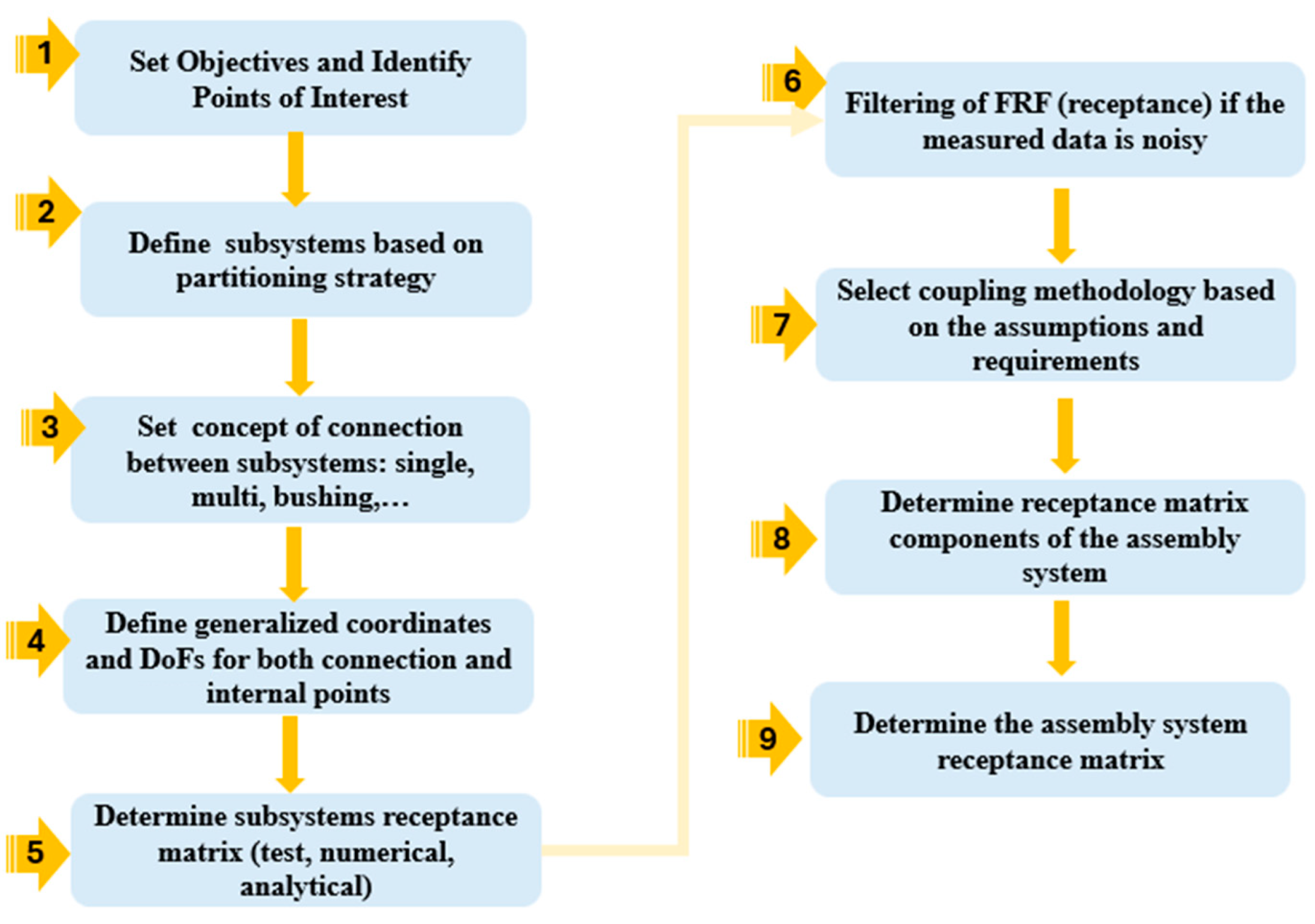
Figure 1. Road map for determining the receptance of the assembly system.
Applsci 14 09550 g001
Figure 2. Assembly of system ABC, comprising substructures A, B, and C, along with their corresponding generalized coordinates and degrees of freedom (DoFs).
Applsci 14 09550 g002aApplsci 14 09550 g002b
Figure 3. Reduction of a three-substructure coupling scheme into a two-substructure system.
Applsci 14 09550 g003
Figure 4. Comparison of receptance components H11, H14, H22, and H33 for frequencies of up to 100 Hz.
Applsci 14 09550 g004
Figure 5. The comparison of receptance components H11, H14, H22, and H33 for frequencies of up to 400 HZ.
Applsci 14 09550 g005
Figure 6. The Substructuring scheme of assembly system AB to two subsystems A and B. (a) Assembly system AB; (b) Generalized coordinates at internal and connection points; (c) Substructuring scheme illustrating the decomposing system AB into subsystems A and B.
Applsci 14 09550 g006
Figure 7. Comparison between three methods for determining receptance components of the system AB.
Applsci 14 09550 g007
Table 1. Material properties and structural parameters used for modeling.
ParametersModulus of Elasticity (E)Moment of
Inertia (I)
Length of Beam
Element (L)
Cross-Sectional Area (A)Section Diameter (d)Density (ρ)
value200 × 109 Pa1.25 × 10−7 m41 m0.0013 m20.04 m7850 kg/m3
Table 2. Lumped parameters for case study 2: model parameters for the 4-DOF system.
Stiffness (N/m) k 1 k 2 k 3 k 4 k 5 k 6
9001300120090011001200
Damping (Ns/m) c 1 c 2 c 3 c 4 c 5 c 6
0.10.20.20.10.20.2
Mass (kg) m 1 m 2 m 3 m 4 m 5 m 6 m 25 m 36
43343366
Disclaimer/Publisher’s Note: The statements, opinions and data contained in all publications are solely those of the individual author(s) and contributor(s) and not of MDPI and/or the editor(s). MDPI and/or the editor(s) disclaim responsibility for any injury to people or property resulting from any ideas, methods, instructions or products referred to in the content.