Abstract
This study presents a generalized and systematic approach to modeling complex dynamic systems using Frequency-Based Substructuring (FBS). The aim is to develop an efficient method for system identification and subsystem decomposition, enabling the creation of reduced-order models for non-linear dynamic systems that are modular and reconfigurable. The methodology combines receptance (Frequency Response Function, FRF) properties from individual subsystems to predict the overall system’s response. This technique extends existing methods by Jetmundsen and D.D. Klerk and adapts them to subsystems with full degrees of freedom (DoFs), making it suitable for flexible and distributed structures. To demonstrate its effectiveness, the method is applied to vehicle noise and vibration analysis, where subsystems are initially treated as rigid bodies, but are later adapted to flexible characteristics. The results show that this hybrid approach accurately predicts system responses, offering significant advantages for NVH target setting when subsystem FRF matrices are sourced either from testing or numerical simulations. This methodology enhances the capability to model complex dynamic systems with improved precision and reduced computational cost. A comparison with traditional modeling techniques confirms the validity of the approach.
1. Introduction
Reconfigurable dynamic systems are increasingly prevalent in industries such as robotics, aerospace, and automotive manufacturing, thanks to their ability to adapt to varying operational conditions and structural configurations. However, accurately predicting the dynamic behavior of these systems, especially during the early stages of development, presents significant challenges due to the complex interactions between subsystems. This complexity is particularly challenging in noise, vibration, and harshness (NVH) analysis, where the dynamic interactions between subsystems often lead to non-linear vibrational responses. In applications such as electric vehicles (EVs), the prediction of these responses early is crucial for appropriate target setting and optimizing vehicle performance and mitigating NVH issues.
Model reduction techniques based on Frequency-Based Substructuring (FBS) and Proper Orthogonal Decomposition (POD) are increasingly used to improve the efficiency of simulation and control for such complex dynamic systems. While system decomposition through receptance coupling methods focuses on dividing a system into smaller subsystems using FBS, which incorporates the full frequency range of dynamic properties through Frequency Response Functions (FRFs), POD relies on mode truncation, specifically targeting the most significant modes to reduce system complexity. However, a primary challenge with POD is the requirement for complete spatial information from the original model to construct the reduced-order model, which can result in significant computational bottlenecks when applied to large-scale systems [1].
To address these challenges, receptance coupling methods using FBS have been developed using coupling Frequency Response Functions (FRFs) of individual subsystems. Initially developed for the coupling of rigid subsystems with fewer degrees of freedom, the original algorithms by Jetmundsen and D.D. Klerk have been widely adopted across various engineering domains.
By transitioning from the time domain to the frequency domain and employing linear properties, this reduced-order modeling approach offers a practical tool for reducing the size of non-linear dynamic systems. This framework integrates FBS with GRC, introducing a systematic technique that facilitates the reliable prediction of dynamic responses in reconfigurable systems. Through the reduction in computational complexity, this methodology effectively simplifies non-linear behaviors, particularly in cases where the study of high-frequency dynamics is important.
This approach has a hybrid feature due to flexibility in leveraging both numerical and experimental data. The proposed approach enhances the modeling capabilities of existing methods, providing a more comprehensive understanding of subsystem interactions and their contributions to overall system behavior. This reduced-order framework is especially valuable in early design stages where limited data are available to develop a detailed model like FEM or MBD.
Two case studies validate the effectiveness of the proposed methodology. The first one presents the analytical derivation of receptance matrix components for a complete vehicle system using a simplified lumped parameter model. The second case study develops a vibrational model for a flexible dynamic structure that can simply be representative of a vehicle’s flexible body structure consisting of three main substructures: the front, middle, and rear end structures. This simple configuration is selected for validation with conventional numerical methods, but this method can be expanded to accommodate more complex dynamic systems with modular and reconfigurable configurations. These studies validate the extended methodology and highlight its practical applications in automotive NVH analysis, where accurate modeling of vibration transfer pathways is essential for optimizing vehicle performance.
Building on foundational work by Bishop and Johnson [2], O’Hara [3], and others, this study consolidates advancements in FBS techniques and extends their applicability to modern engineering challenges.
Numerous studies have since explored the dynamic characteristics of systems composed of interconnected substructures, frequently utilizing dynamic substructuring techniques with FRF data. In 1985, Ewins and Gleeson [4] proposed a method to identify the modal properties of structures using FRFs to derive system parameters.
Among FBS approaches, the generalized receptance coupling method introduced by Jetmundsen in 1988 [5] and the Lagrange multiplier Frequency-Based Substructuring (LM FBS) method introduced by De Klerk et al. in 2006 [6] stand out as widely adopted techniques. These methods extend to the substructure decoupling problem, which is essential for determining the dynamic response of subsystems from the overall system. However, the novel contribution of this paper lies in applying these methods to non-linear dynamic systems through a reduced-order approach in the frequency domain, facilitating more accurate and computationally efficient predictions.
Recent advancements have further refined FBS techniques. in 2017, Zhang, Song, and Xu [7] employed FBS to investigate the dynamic behavior of subframes assembled with vehicle bodies. In 2019, Kang et al. [8] introduced a method for deriving a road noise improvement factor within suspension systems using inverse substructuring, demonstrating the efficacy of FBS in practical automotive applications. In 2020, Hülsmann, Van der Seijs, and their team at BMW Group and VIBES.technology [9] demonstrated the application of dynamic substructuring in electric car drivetrain design, focusing on NVH issues.
Further research by Tsai in 2019 [10] extended methods for measuring rotational receptance, a key factor in accurately estimating rotational dynamics. In 2017, Clontz and Taheri [11] focused on decoupling tire subsystems from suspension subsystems using FBS techniques, contributing to advancements in automotive NVH modeling. In 2022, Voormeeren and Rixen [12] investigated the impact of uncertainties in substructure measurements on FBS outcomes, emphasizing the need for precision in measurements. In 2021, De Klerk, Rixen, and Jong [13] introduced new algorithms to enhance the accuracy and reliability of FBS when coupling subsystems, contributing to the growing body of work aimed at refining FBS methodologies. De Klerk et al. (2009) present a general framework for dynamic substructuring, classifying various methods developed over four decades, with an emphasis on dual and primal assembly approaches. This framework helps understand the mathematical foundations of substructuring techniques and addresses current challenges in experimental dynamic substructuring [14]. Their work builds on earlier research by Liu and Mir in 2003 [15], which introduced experimentally validated hybrid methods for vehicle axle noise simulation.
In 2021, Li et al. [16] explored dynamic substructuring in railway vehicle dynamics, showcasing FBS’s versatility across different industries. Similarly, in 2020, Scheel and Sturzenegger [17] applied FBS to the aerospace sector, focusing on the dynamic analysis of satellite structures. Additionally, in 2022, Nguyen et al. [18] examined the application of FBS in the context of robotic systems, particularly in modular robotic configurations. The evolution of FBS techniques is further evidenced by the work of Gebhardt et al. in 2020 [19], who utilized FBS for dynamic analysis in wind turbine blade structures, and that of Park et al. in 2023 [20], who applied FBS in the marine industry, focusing on ship hull vibration analysis. The recent work of Lee et al. in 2021 [21] explored FBS for the dynamic analysis of civil engineering structures, such as bridges and high-rise buildings, highlighting its expanding relevance. Recent studies have demonstrated the effectiveness of multi-body dynamic modeling and substructuring techniques for optimizing vehicle vibration and noise control, especially in body mounting systems. El Mahmoudi et al. (2019) focused on optimizing joint parameters within the LM-FBS framework, using automotive rubber bushings as a case study, showing how changes in parameters, such as those in engine mounts and suspension systems, influence system sound pressure [22]. Kang et al. (2019) employed FBS to reduce road-induced excitation at the body mounting interface, using an inverse substructuring method to estimate the dynamic stiffness modification of bushings for road noise reduction [23].
Since the foundational work of Jetmundsen and D.D. Klerk, the field of FBS and receptance coupling has seen significant advancements. Recent developments have expanded these early contributions by integrating novel methodologies and technologies. Notably, Schmitz et al. (2022) introduced a sophisticated approach that combines receptance coupling substructure analysis (RCSA) with Bayesian machine learning for milling stability predictions [24]. Albertelli et al. (2013) did consider rotational DoFs in their improved RCSA methodology. This approach incorporates both translational and rotational dynamics in estimating the system’s full receptance or FRF matrix. By doing so, it helps predict chatter-free cutting conditions at high frequencies, which is crucial for ensuring stability in high-speed machining processes [25].
Additionally, Hamedi and Taheri (2024) provided a fundamental review of hybrid and modular modeling features and substructuring schemes using RCFBS, highlighting the effectiveness of these techniques for predicting road noise and vibrations in vehicle dynamics [26]. In another study, Hamedi and Taheri (2024) demonstrated that the receptance coupling Frequency-Based Substructuring (RC-FBS) method offers superior accuracy for high-frequency dynamics, particularly in systems with flexible or distributed parameters. Their findings reveal that the RC-FBS method achieves stronger alignment with finite element analysis (FEA) and direct solution techniques compared to traditional modal analysis, largely due to mitigating mode truncation issues common in modal approaches. Additionally, RC-FBS provides more precise results during the decomposition process, particularly when subsystems exhibit significant flexibility, and excels in predicting both rotational and translational dynamics in complex systems. These capabilities make RC-FBS a significant advancement for modeling dynamic systems across high-frequency domains [27]. The authors extend the application of this method to the development of a half-vehicle model, enabling modular coupling of dynamic interactions between subsystems like the chassis and suspension. By consolidating substructures like the front and rear suspensions into a single module with a sparse matrix representation (minimizing off-diagonal term inversions), this method reduces unnecessary computational complexity and enhances model reliability. This model reduction strategy can also minimize potential noise from off-diagonal elements appearing in experimental data, preserving boundary conditions and improving stability for practical, computationally efficient applications [28].
The novelty of this paper lies in advancing the field of FBS and generalized receptance coupling Frequency-Based Substructuring (GRCFBS) by addressing key challenges and expanding their applicability to NVH modeling. One major contribution is the scalability of the GRCFBS method, which extends a unified coupling framework to accommodate diverse subsystem configurations while maintaining the same number of substructures and interface mappings. This scalability enables flexible applications critical for NVH tasks, such as target setting, cascading, system identification, and subsystem decomposition. For example, the framework is applied to electric vehicle (EV) suspension systems with varying subsystem configurations, such as the trimmed body–suspension–tire configuration with rigid connections and the subframe-trimmed body–electric motor configuration with elastic mounts. Both configurations share an identical subsystem architecture and interface mapping, demonstrating the standardized approach’s capability to model reconfigurable systems with modular and hybrid configurations.
Another key contribution of this work is the efficient integration of both translational and rotational DoFs within the LM-FBS method. This advancement addresses a significant challenge in FBS, broadening its applicability to systems with complex dynamic interactions while maintaining computational efficiency. The approach has been validated using traditional numerical methods, confirming its reliability for high-frequency NVH applications, which are often computationally demanding and require precise modeling techniques. Additionally, this paper compares the Jetmundsen and LM-FBS methods, demonstrating their equivalent coupling formulation useful for predicting road noise transmission for vehicle NVH models. Finally, this work extends GRCFBS to address the unique NVH challenges of electric vehicles, such as motor-induced vibrations and tire–road noise. The proposed methodology effectively captures both low- and high-frequency behaviors, enabling reliable predictions of cabin noise and facilitating early-stage NVH analysis and design optimization for EV systems. These advancements establish an efficient framework for dynamic system modeling, applicable across industries where noise, vibration, and structural dynamics are critical considerations.
2. Method
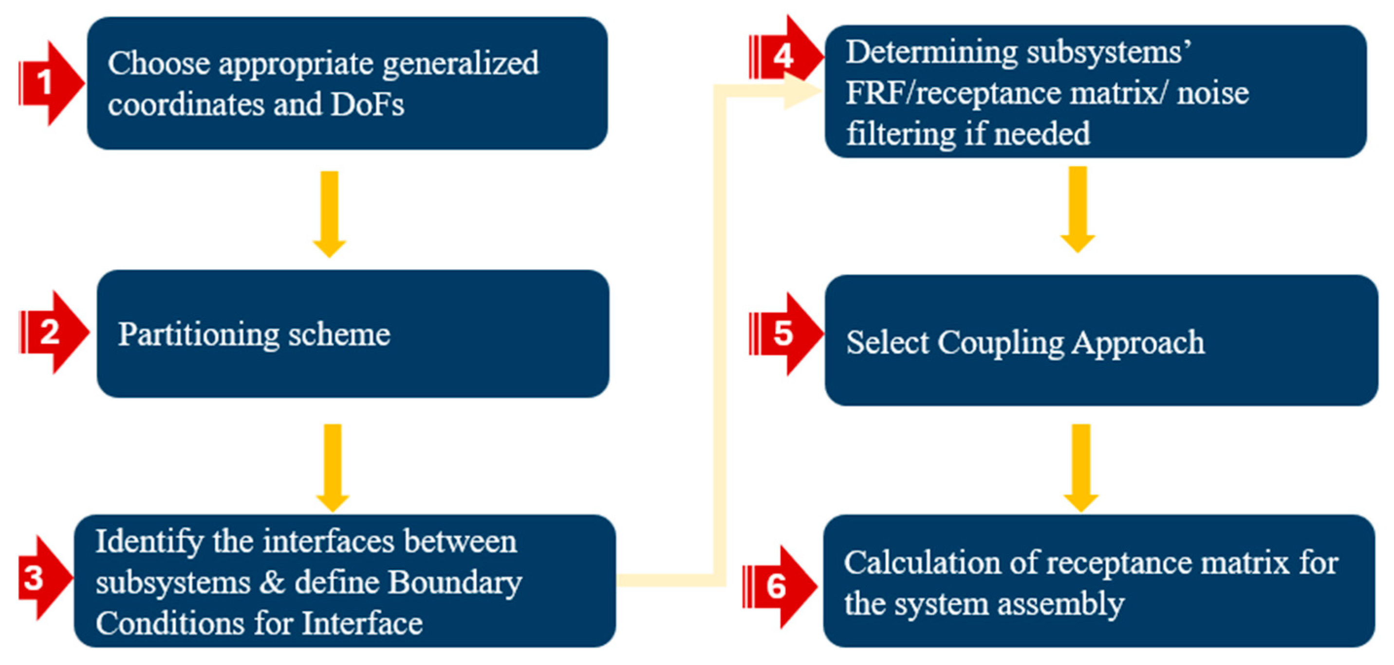
To effectively model reconfigurable dynamic systems, a structured, step-by-step approach is essential. Firstly, appropriate measurement points and DoFs are selected, with emphasis on both interface and interior points of the substructures to capture necessary data. The system is then partitioned into manageable substructures based on available subsystem data and design requirements, facilitating a more feasible analysis of the system’s dynamic behavior. Boundary conditions are established at the interfaces between subsystems, ensuring compatibility and equilibrium while considering factors like single or multiple connection points and interface flexibility. Next, each disassembled subsystem undergoes modal analysis to determine its FRF matrix at the free–free condition, which can be derived through finite element analysis (FEA), analytical methods, or experimental techniques. After obtaining individual FRFs, a suitable coupling approach is selected to integrate these subsystem models into a system model; options include impedance coupling, receptance coupling, Jetmundsen’s approach, and LM-FBS coupling, depending on system complexity and required accuracy. Finally, the receptance matrices of individual substructures are synthesized using the chosen coupling method to create a cohesive model representing the dynamic behavior of the entire system. This structured approach, summarized in Figure 1, provides a roadmap for modeling reconfigurable dynamic systems using a generalized coupling method with Frequency-Based Substructuring (FBS).
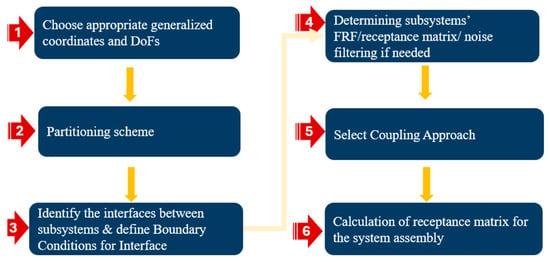
Figure 1.
Flowchart describing the road map for modeling of reconfigurable dynamic systems using generalized coupling method.
The proposed methodology offers several key advantages, particularly for reconfigurable dynamic systems with modular-based configurations. It simplifies the analysis of complex systems through reduced-order models by combining receptance points that represent measurement and excitation points, such as those in suspension systems, without requiring geometrical complexity. This improves accessibility while maintaining accuracy. By integrating experimental and analytical data, it enhances prediction precision and reduces errors, particularly at subsystem interfaces. The method also facilitates early-stage NVH modeling, delivering critical insights—especially in vehicle electrification, where tire–road noise has become a primary source of cabin noise. Additionally, it provides explicit tools for cost-effective subsystem coupling and decomposition, enabling accurate noise prediction and system performance optimization.
The methodology is highly adaptable, supporting straightforward updates to individual components without requiring a complete system redesign, making it ideal for iterative design processes. Its focus on modular-based configurations allows for the efficient analysis and refinement of individual subsystems, making it particularly well-suited for reconfigurable systems. It also has potential to simplify the analysis of systems with local non-linear components by treating non-linear behavior within subsystems while maintaining linear assumptions at connection points through compatibility and equilibrium. Non-linear dynamics can be incorporated as additional dynamic stiffness or experimental receptance measurements modeled as black-box subsystems. This modular approach enables the targeted refinement of non-linear substructures without necessitating the reanalysis of the entire system, offering significant computational efficiency and flexibility in design and analysis.
3. Theory
Frequency-Based Substructuring (FBS) systematically analyzes the dynamic behavior of reconfigurable dynamic systems by breaking down the system into smaller, more manageable subsystems. This methodology uses frequency-domain coupling to integrate subsystem transfer functions obtained either numerically or experimentally, enabling the creation of hybrid models. By measuring FRFs at critical points, particularly at interface coordinates, engineers can develop effective reduced-order models that accurately capture the subsystem interactions without requiring detailed geometrical complexity.
The FRF or receptance matrix can be measured experimentally through experimental methods such as impulse hammers or shakers for structure-borne vibration analysis, and loudspeakers or volume velocity sources for airborne noise analysis. These measurements are limited to disassembled subsystems, improving access to connection points and reducing the overall measurement burden. In real-world situations where there are lots of interference signals, FRFs are calculated using power spectral density (PSD) and cross-power spectral density (CPSD), which mitigate noise and improve precision.
For structural vibrations, a dynamic system comprising interconnected subsystems is governed by the equilibrium between externally applied forces and internal forces. The equation of motion for each subsystem is as follows:
where , , and represent the mass, damping, and stiffness matrix of i-th subsystem, respectively. The vectors and denote the generalized response and external excitation force, respectively. By applying the Fourier transform, the dynamic response in the frequency domain can be expressed as follows:
where is the dynamic stiffness (impedance matrix), and represents the FRF or receptance matrix for the i-th substructure. An element of the FRF matrix, , is defined as the partial derivative of the response at the i-th generalized coordinate with respect to the excitation force applied at the j-th point:
Using partitioning method, the equations of motion for the j-th substructure of the system are expressed in matrix notation as follows:
In this context, subscripts i and c denote internal and connection DoFs, respectively. The term represents the receptance matrix, which can be determined by applying an excitation force at the internal measurement points and measuring the resulting displacements at the same points. Similarly, is determined on isolated substructure j by applying an excitation force at the interface or connection measurement point and measuring the resulting response at the internal point . Due to the symmetric nature of the receptance matrix, commonly referred to as reciprocity, . Assuming n arbitrary subsystems are coupled, the overall equations of motion for the dynamic system can be written as follows:
This equation can be simplified as follows:
where represents the additional unknown interface forces connecting the subsystems, ensuring equilibrium at the interface points. In the frequency domain, the dynamic equilibrium is expressed as follows:
In matrix notation, this can be expressed as follows:
Next, the assembly boundary conditions between subsystems must be applied. These constraints, along with compatibility equations, must be satisfied to represent the coupling condition. The next section of this paper discusses the approaches for coupling the substructures.
4. Procedures
The initial step of this methodology begins with determining decoupled receptance matrices for individual substructures, while these are combined during the coupling process through equilibrium and compatibility conditions, creating a unified matrix that reflects the interactions and dependencies between substructures. This step transitions the model from an isolated mathematical representation to a realistic system-level model. The mathematical coupling process is designed to account for the interaction between substructures at their interfaces. This includes both rigid and flexible connections, with the latter being modeled through interface compliance. This ensures that the resulting coupled system better reflects the real physical interaction between substructures. The coupling methodology has been validated in prior experimental studies (e.g., using a small-scale quarter car model) and was shown to accurately predict the dynamic response of coupled systems. This confirms that the mathematical coupling formulation represents real substructures when experimental or numerically derived FRFs for the involved subsystems are used. The receptance matrices themselves can be obtained experimentally, analytically, or from the FEA of the individual substructures, ensuring they reflect the real physical properties of the subsystems. In the case study here, substructure receptances have been obtained from numerical FEA.
4.1. Receptance Coupling Algorithms
This section discusses two established generalized receptance methods: LM-FBS and Jetmundsen algorithms. Both methods are widely used for coupling multiple subsystems or substructures through interface boundary conditions. While the LM-FBS method utilizes Lagrange multipliers to enforce equilibrium and compatibility between coupled substructures, the Jetmundsen method offers a less explicit representation of interface forces.
4.1.1. D.D. Klerk Algorithm (LM FBS)
The LM-FBS method integrates Lagrange multipliers (λ) to ensure equilibrium and compatibility between coupled substructures. The equations of motion for rigid and flexible coupling scenarios are presented in the following [14]:
- Rigid Coupling Considerations
In the rigid coupling case, the interface points between the connected substructures have no relative motion, simplifying the compatibility condition. The displacements at these interface points are identical across substructures, allowing for a straightforward prediction of the system’s dynamic behavior. The equilibrium equation for the rigid coupling scenario is as follows:
where [B] is a Boolean mapping matrix that enforces compatibility conditions on the interface DoFs. Here, and represent interface forces and generalized coordinates for points of interest, respectively. The matrices [L] and [B] are orthogonal, such that , ensuring interface equilibrium. The dynamic stiffness matrix [Z] is the system’s impedance matrix, and is the receptance matrix. The Lagrange multipliers λ are expressed as follows:
Substituting Equation (10) into Equation (9), the coupled receptance matrix of the system assembly is obtained [13]:
Figure 2 illustrates FBS method for assembling substructures A and B, depicting the interface forces λ used in the LM-FBS method.

Figure 2.
Coupling of two subsystems A and B with both internal and connection DoFs and the interface forces λ.
- Flexible Coupling Considerations
When interface compliance is introduced, relaxing the strict compatibility condition better captures the dynamic behavior of interconnected subsystems. As noted by Bishop and Johnson [1], this relaxation of compatibility is essential for the accurate prediction of flexible interfaces. The equations of motion for flexible coupling are as follows:
where is the impedance matrix for the flexible mounting system, which accounts for the stiffness, damping, and mass matrices of the mounting system:
If a flexible coupling exists at the interface between substructures, the flexibility at the interface contributes to the overall interface dynamic stiffness. Consequently, the interface forces λ are given by the following:
This leads to the modified coupled receptance matrix:
The interface forces λ ensure compatibility between substructures, maintaining the balance of the system.
The LM-FBS method, however, offers enhanced robustness under noisy or inaccessible interface conditions, making it particularly advantageous for experimental NVH modeling and determining internal forces at interfaces. Despite these strengths, its dependence on the mapping matrix [B], which defines interface compatibility, can pose challenges in systems with complex non-linear interface dynamics, underscoring the need for careful consideration in practical applications.
4.1.2. Jetmundsen Algorithm
Based on the assembly of two substructures with internal and connection DoFs, as illustrated in Figure 2, the equations of motion for the disassembled substructures A and B can be expressed as follows:
where “a” and “b” denote the interior DoFs of substructures A and B, and “c” denotes the connection DoFs. The equations of motion for the coupled system are given by the following:
Using the compatibility principle , , , along with the equilibrium principle , Jetmundsen derived the following coupled receptance matrix for the assembly of substructures A and B:
In Equation (18), the term represents the coupling receptance at the connection points between the two substructures. If there is a bushing or flexibility at the interface, the bushing receptance , which is inverse of the dynamic stiffness, can be incorporated as . This formulation has already been generalized for coupling of N arbitrary substructures using the following:
In this equation, [] is a Boolean mapping matrix that describes the interconnections between substructures. The s-th row of [], denoted as , represents the connections of a specific substructure to others. and represent the partitioned receptance matrices for the internal and interface DoFs, respectively. This framework enables systematic coupling of multiple substructures, using graph theory to analyze complex dynamic systems. The symbol ⊗ denotes the Hadamard product, which applies the element-by-element product. The elements of [] establish the sign convention for interfaces: “+1” or “−1” is assigned based the directionality of connected interfaces, while “0” indicates no connection between a subsystem and the interface path [29].
4.2. Case Studies
This section presents the application of the proposed methodology through two case studies. The first case focuses on the development of an analytical NVH model of a car to determine the receptance matrix of the entire system based on the receptance components of individual subsystems using both coupling algorithms. The primary objective is to develop an effective reduced-order model that evaluates noise transmission from road surfaces and electric motors to the vehicle body. The second case involves the numerical modeling of a dynamic structure composed of three substructures. This system is modeled as a free–free beam, consisting of three beam elements, with each element representing a distinct subsystem.
4.2.1. Analytical Coupling Approach for Vehicle Vibration Analysis
In this case study, an analytical framework is developed for modeling vehicle vibration, using a simplified quarter car model. The model consists of three interconnected substructures: the vehicle’s trimmed body (substructure A), the suspension system (substructure B), and the wheel assembly (substructure C), as illustrated in Figure 3. These substructures are connected through two interfaces c1, connecting the body and suspension, and c2, connecting the suspension and wheel. The system is defined by the following DoFs: substructure A, the trimmed body subsystem, is modeled with two DoFs: one internal DoF , representing the reference measurement point within the cabin, and an interface DoF , corresponding to the connection point with the suspension. Substructure B, the suspension subsystem, is modeled with three DoFs: one internal DoF and two interface DoFs, and , connecting to the body and wheel, respectively. The wheel assembly, substructure C, has two DoFs: at the hub center, treated as an internal DoF, and at the spindle attachment.
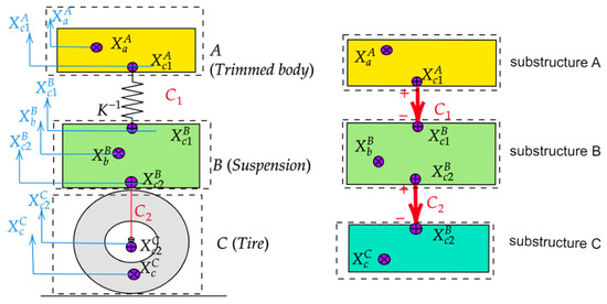
Figure 3.
Coupling of three substructures for road noise prediction.
The objective is to derive the governing equations for predicting the vehicle body’s vibrational response to external excitations, such as road and electric motor operations. Both the Jetmundsen and D.D. Klerk algorithms are employed, utilizing the receptance matrices of the individual substructures. The resulting coupled system response is obtained by combining the individual substructure responses via the interface boundary conditions.
Use of Jetmundsen Coupling Algorithm
The Jetmundsen method, expressed in Equation (18), partitions the receptance matrices of the substructures and uses graph theory for system assembly [30]. The corresponding matrices , , , and , which are derived based on the substructures’ DoFs and their connections, are outlined in Equations (20) and (21):
where the DoFs α for the substructures are .
The mapping matrix , describing the interconnections between substructures, is defined as follows:
Partitioned matrices correspond to the connections between substructures:
There is no connection between substructure C and interface c1 and between substructure A and interface c2 and . These relationships simplify the formulation of the coupling matrix. Therefore is obtained as follows:
Subsequently, is derived as follows:
As a key component of the assembly system’s receptance, the coupling receptance between substructures is calculated in Equation (25).
The resulting coupled receptance matrix, , is calculated by substituting Equations (20)–(24) into Equation (19). It accounts for dynamic stiffness at the interfaces and the flexible effects of bushings or mounts:
it should be noted that the interface c2 between the tire and suspension has been considered rigid due to bolted fixation. However, the suspension is connected to the body via bushings or mountings, which necessitates integrating the effects of bushing compliances at the interface c1 through the dynamic stiffness of the bushing K.
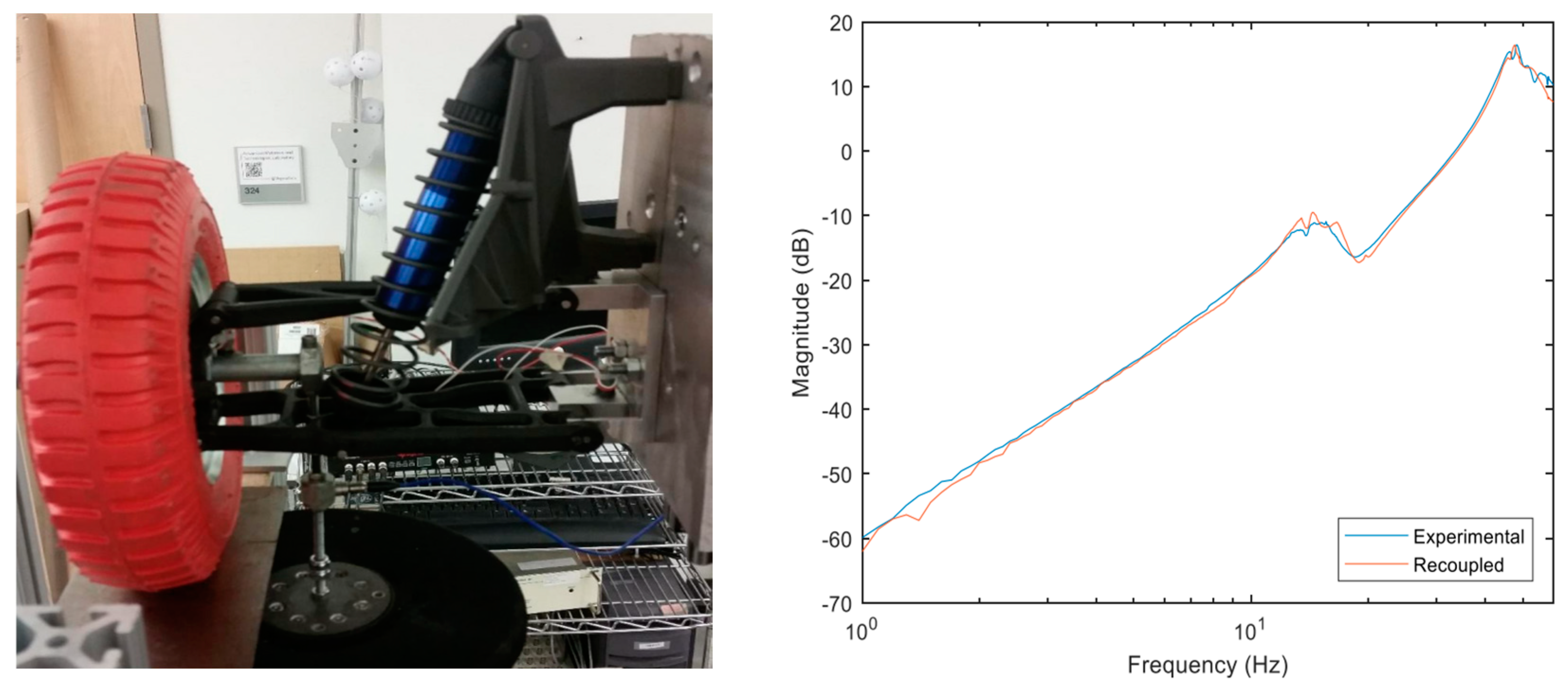
The receptance coupling method was previously validated through experimental work conducted at our lab (CenTiRe) using a small-scale quarter car model, consisting of both the suspension and tire. Figure 4 illustrates the physical setup and the comparison between the experimentally obtained receptance and those derived from coupling the tire and suspension. The maximum discrepancy between the natural frequencies predicted by the coupling and the experimentally observed values was 6.6% in natural frequencies, mostly due to deflection in the suspension components (Clontz, 2018) [31]. This close alignment of experimental and predicted results reinforces the robustness of the methods developed in the present study.

Figure 4.
Comparison of receptance for the assembled quarter car system obtained experimentally and through coupling of tire and suspension [31].
Use of LM-FBS Coupling Algorithm
To apply this framework, we start by determining the Boolean matrix that satisfies the compatibility conditions, ensuring that displacements are equal at interface connection points. In this context, [H] is analogous to [Hαα] from the previous method. The boundary conditions at the interfaces are expressed as , ensuring compatibility between the degrees of freedom (DoFs) at the interface coordinates. These conditions align the displacements at connection points, as enforced by the Boolean matrix.
and {X} represents the displacement vector of the DoF coordinates corresponding to measurement points of interest: .
It is important to note that Equation (25) is derived by assuming a rigid interface, and it is not valid in the context of a non-rigid connection between substructures A and B. In the case of flexible coupling, the Boolean matrix would be determined from Equation (12). The next step involves calculating the following:
By substituting the matrices in Equation (27) into Equation (15) and further refinement during matrix operations, the final expression for the coupled system’s receptance is obtained as follows:
By comparing the results from the Equations (25) and (28), both the Jetmundsen and LM-FBS methods produce identical outcomes for the coupling of three substructures. Hence, both approaches provide effective coupling models to predict road noise transferred to the vehicle body based on the receptance transfer functions of the decoupled subsystems, i.e., A (trimmed body), B (suspension), and C (tire). These functions can be either measured experimentally or obtained through free–free vibration tests or finite element analysis (FEA). Finally, the resulting equations of motion for the coupled system ABC can be represented in matrix notation as follows:
In Equation (29), is a symmetric matrix with a rank of , and can be derived from one of the coupling algorithms, i.e., Equation (25) or Equation (28). This equation can be reformulated to facilitate determining the response of the system vector with respect to any arbitrary vector of excitation forces as follows:
In this matrix, for instance, term represents the direct receptance of the assembly system ABS, where the excitation force is applied at the connection c1 on substructure A, and the response is measured at the same connection point.
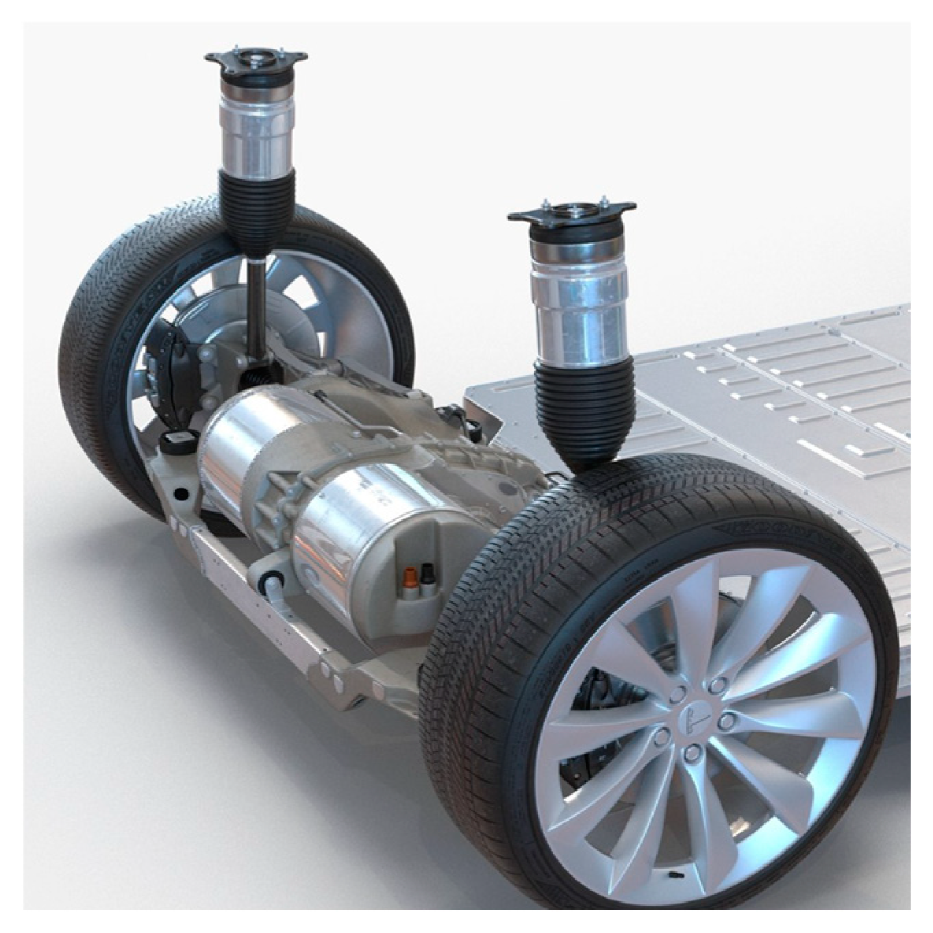
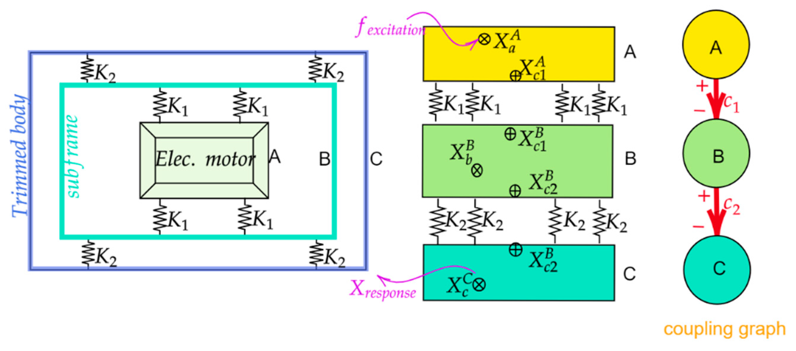
This approach enables the prediction of the vehicle’s vibrational and acoustic response to various excitations, providing an analytical framework for understanding noise transmission within the EV structure. For electric vehicle (EV) applications, the three-substructure scheme is used to predict noise transfer to the cabin, especially noise originating from the EV motor integrated into the suspension subframe. In this scenario, the substructures are defined as the vehicle body, the suspension subframe, and the EV motor, which is presented for a Tesla Model S chassis, as demonstrated in Figure 5. For such dynamic systems, the three-substructure coupling formulations, as given in Equation (25) or (28), can be used to determine the receptance of the assembled system (ABC) based on the receptance of the decoupled subsystems, as shown in Figure 6. In this case study, the bushing elements between the subsystems necessitate adjustments to the receptance matrix at the connection points. This adjustment incorporates the bushing receptance and is expressed by the following formula:
where represent the dynamic stiffness of the mountings between subsystems A and B, and between subsystems B and C, respectively. It is important to note that the dynamic stiffness values K1 and K2 in Equation (31) and K in Equations (25)–(28) are included as general parameters representing the stiffness of the mountings between subsystems. As this study focuses on the theoretical development of the receptance coupling formulation, specific numerical or experimental values for mounting stiffness have not been assigned. These parameters are expected to be determined based on the material properties, geometry, and operating conditions of the system in future applications.

Figure 5.
Tesla Model S chassis 2; image retrieved from TurboSquid [32].

Figure 6.
Vibrational model of EV suspension assembly using receptance coupling and three substructures.
4.2.2. Numerical Modeling of a Dynamic Structure
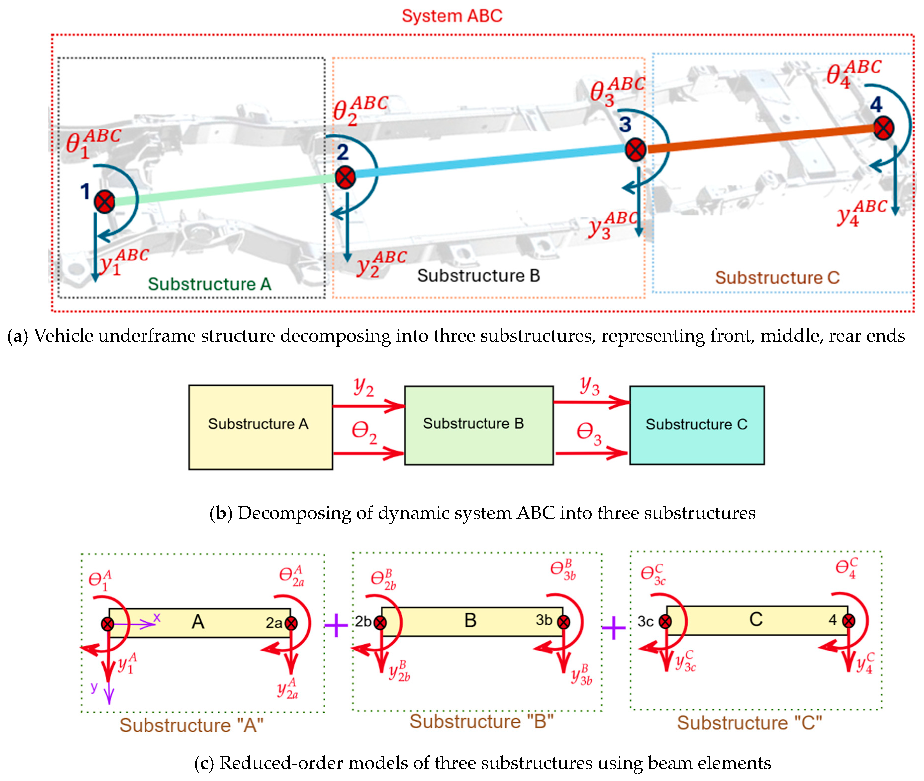
This case study analyzes a simplified dynamic structure consisting of three interconnected substructures, as shown in Figure 7. The model incorporates two connection points, labeled 2 and 3, with each connection point having two DoFs: one translational and one rotational, due to the use of beam elements in a 2D plane. The system is modeled as a free–free structure with three beam substructures, which can serve as a simplified representation of a vehicle structure—comprising the rear, middle, and front sections, as shown in Figure 7a. The analysis is performed using the generalized coupling method, with the results compared to those obtained from numerical finite element analysis (FEA) and modal analysis. To ensure simplicity and consistency in the DoFs across all methods, each substructure is modeled as a single beam element with uniform properties.
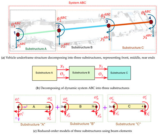
Figure 7.
Dynamic structure consists of three substructures with beam element.
The key assumptions are as follows: (1) the system exhibits linear dynamic behavior, with no non-linearities in stiffness or mass; (2) the analysis is conducted for an undamped system to focus on the coupling method and its comparison with existing undamped models; (3) subsystems A, B, and C are rigidly coupled without flexibility at the connections; (4) no geometric non-linearities or large deformations are considered; (5) the receptance data for each subsystem are assumed to be known, and in the case study presented, the substructure receptances are captured using an analytical method based on the stiffness and mass matrices of beam elements which are representative of subsystems; and (6) the frequency range is assumed to capture primarily flexible modes without higher-order complexities.
Generalized Coupling Method Using LM-FBS
The dynamic system, denoted as ABC, is divided into three substructures, as shown in Figure 7b. To apply the LM-FBS algorithm, the Boolean matrix is constructed to satisfy the compatibility conditions at the interface connection points, ensuring equal displacements at the interface connection points. The boundary conditions at the interfaces can be expressed as follows:
Using these compatibility conditions, the Boolean matrix [B] is formulated based on the DoFs at the interface coordinates, as shown in Equation (33):
The generalized displacement vector {X}, which encompasses the DoFs of internal nodes and connection points, is expressed as follows:
The receptance matrix for the coupled system ABS is assembled as follows:
In Equation (35), the receptance matrix for each substructure i (A,B,C) is calculated from , where and are the mass and stiffness matrices of substructure i, derived from the beam element formulation in Equations (36) and (37).
Figure 7c shows the dynamic structure, consisting of three substructures modeled using beam elements as well as a substructuring scheme and the interested generalized coordinates and DoFs, while Table 1 summarizes the material properties and structural parameters used for simulation.

Table 1.
Material properties and structural parameters used for modeling.
Validation of the GRC-FBS Method
To validate the GRC-FBS method, its results are compared to those obtained from the numerical FEA and modal analysis. The receptance matrix from the numerical FEA is calculated by modeling each substructure individually. To ensure consistent DoFs across all methods, each substructure is represented as a single beam element despite the higher discretization typically required for beam models.
The subsystems A, B, and C are modeled using their stiffness and mass matrices and for all three beam elements, as expressed in Equations (35) and (36) [33,34]. This simplification ensures consistency and reduces computational complexity. The local stiffness and mass matrices for each substructure are defined as follows:
The global receptance matrix of the assembly system AB, is computed as follows:
where and are the global mass and stiffness matrices, which are calculated by combining the stiffness and mass matrices of the three elements.
For the modal analysis, assuming an undamped system, the components of the receptance matrix are determined using [35]:
Here, is natural frequency of the r-th mode, is the normalized mode shape at , and n represents total number of DoFs or modes. Given the configuration of the problem—three elements and four nodes, each with rotational and translational DoFs—the system has eight DoFs. The natural frequencies for this free–free beam system are presented in Table 2. Since the results from the three methods are closely aligned, they are not separately listed in the table.

Table 2.
The natural frequencies for the free-free beam system ABC.
The mode shapes are the eigenvectors corresponding to the natural frequencies, obtained by solving the eigenvalue problem:
The normalized mode shapes are computed as follows:
4.3. Ill-Conditioning in Coupling Methods
Noise in measuring the FRFs of subsystems poses significant challenges to coupling methods, leading to ill-conditioned matrices that compromise the stability and accuracy of matrix inversion operations, especially in nearly singular matrices, where errors are amplified during inversion. A rank deficiency may occur due to linear dependence among rows or columns, frequently due to insufficient measurements. Disparities in the dynamic characteristics of coupled subsystems, such as differences in stiffness or damping, can cause wide-ranging eigenvalues and numerical instability. High-frequency effects further exacerbate sensitivity to minor data inaccuracies, while poorly chosen interface DoFs might fail to capture essential dynamics, resulting in ill-conditioned matrices. Additionally, closely spaced natural frequencies can render matrices nearly singular, complicating the inversion process.
To address these challenges, recent studies have explored methods to enhance the accuracy and stability of matrix inversions. Luo et al. [36] proposed a regularization method specifically designed for FRF-based substructuring, which complements the use of Singular Value Decomposition (SVD) in mitigating noise-related issues. Similarly, Zheng et al. [37] applied Tikhonov regularization alongside the pseudo-inverse method to improve inverse force identification, illustrating ongoing efforts to refine mathematical tools in the face of real-world measurement inaccuracies. In coupling methods, non-square matrices may arise, particularly when subsystems with different degrees of freedom are involved. These matrices, representing relationships between input and output variables such as receptance matrices or transfer functions, often lack invertibility. For an ideal scenario with excitations and corresponding responses, the receptance matrix is square and invertible. The inversion equation is expressed as follows:
However, when dealing with excitation forces and measurement responses, the challenge involves due to inverting a rectangular, rank-deficient receptance or FRF matrix . In this case, the pseudo-inverse matrix approximates the inverse:
The pseudo-inverse matrix is computed as follows:
To address noise in measured data, techniques such as regularization or SVD are often preferred, which decompose the data matrix into singular vectors and singular values, filtering out noise by focusing on dominant modes of variation. The core principle of SVD involves expressing matrix H as , where U and V are orthogonal matrices, and S is a diagonal matrix containing singular values . If H is singular or ill-conditioned, its inverse can be approximated by the pseudo-inverse In this formulation, represents the pseudo-inverse of the singular values matrix. By setting small singular values to zero, SVD effectively mitigates issues related to ill-conditioned matrix inversions, particularly when input FRFs are significantly affected by noise [38,39,40,41].
In practical applications, mitigating ill-conditioning often involves preprocessing FRF measurements, such as spectral averaging or cross-power spectral density calculations, and carefully selecting interface DoFs to capture dominant dynamic behaviors. While these considerations were not explicitly incorporated into the case studies in this paper, they are critical for extending the methodology to more complex, real-world systems.
5. Results
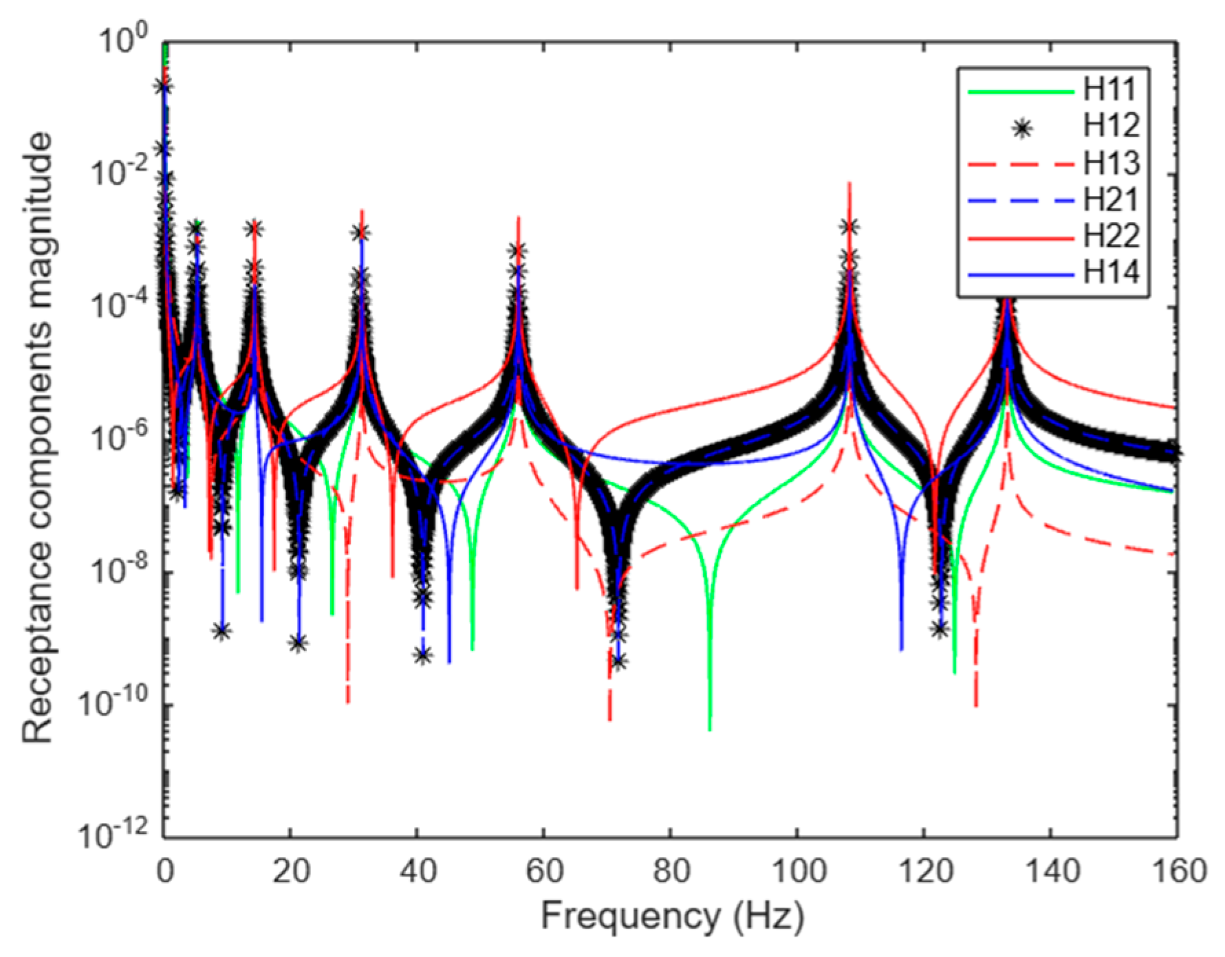
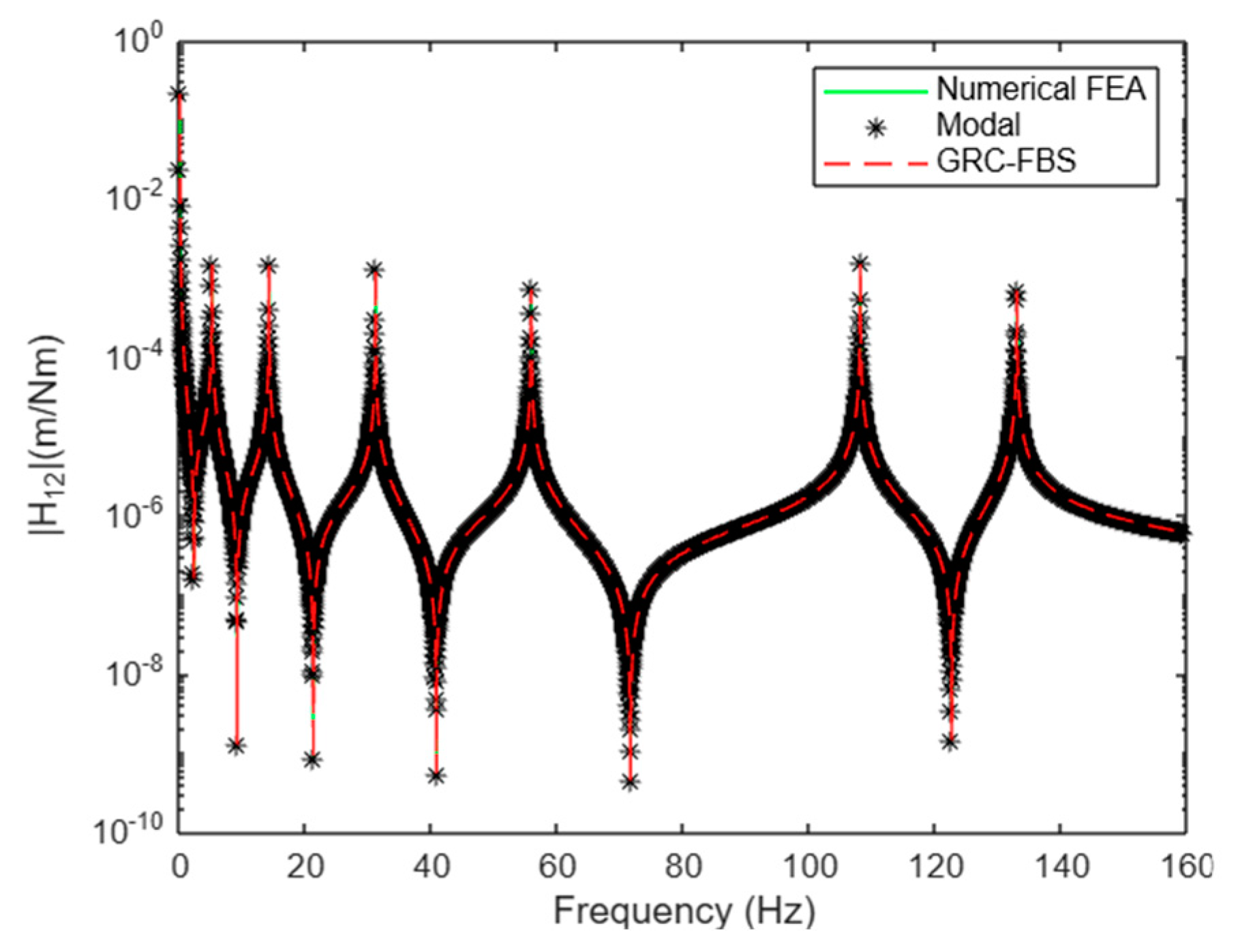
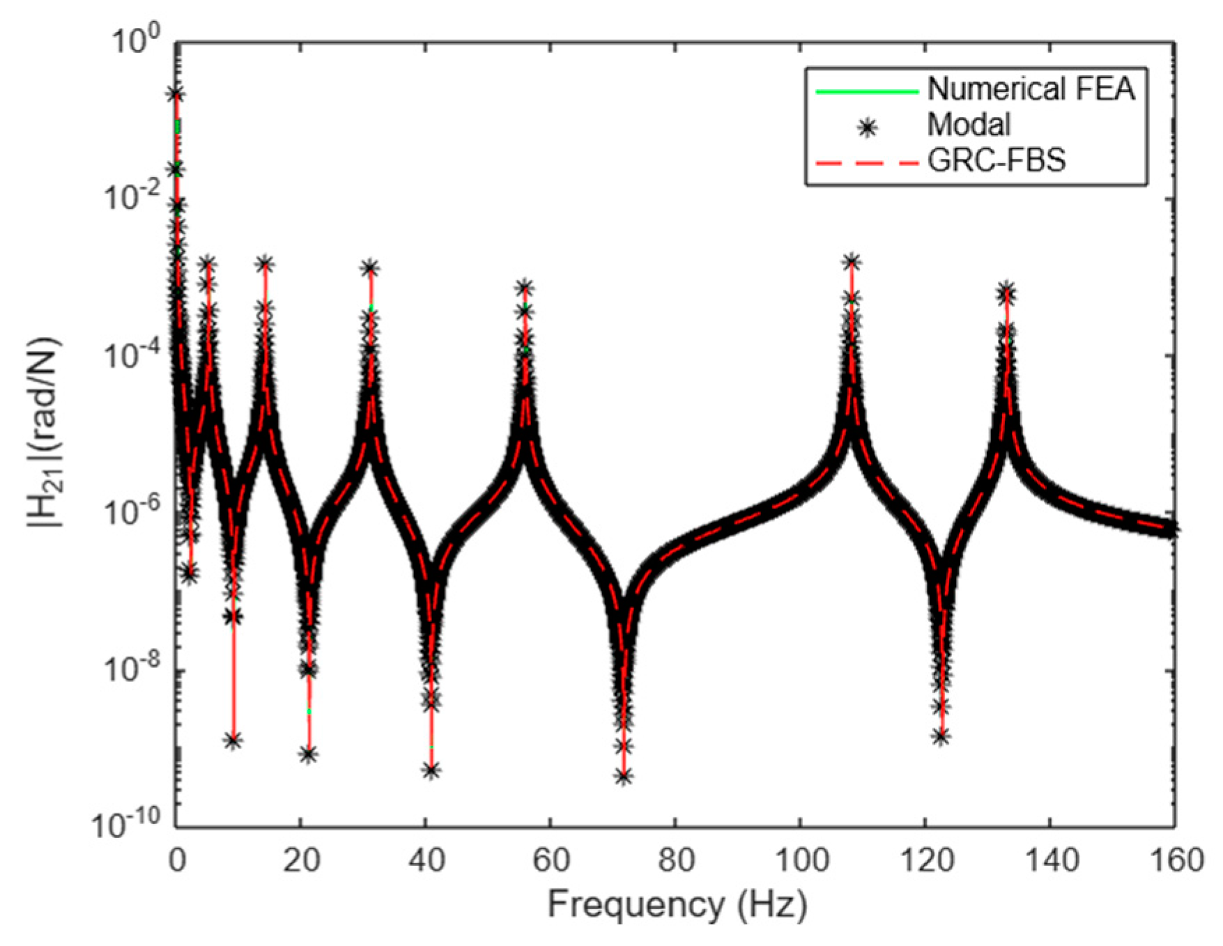
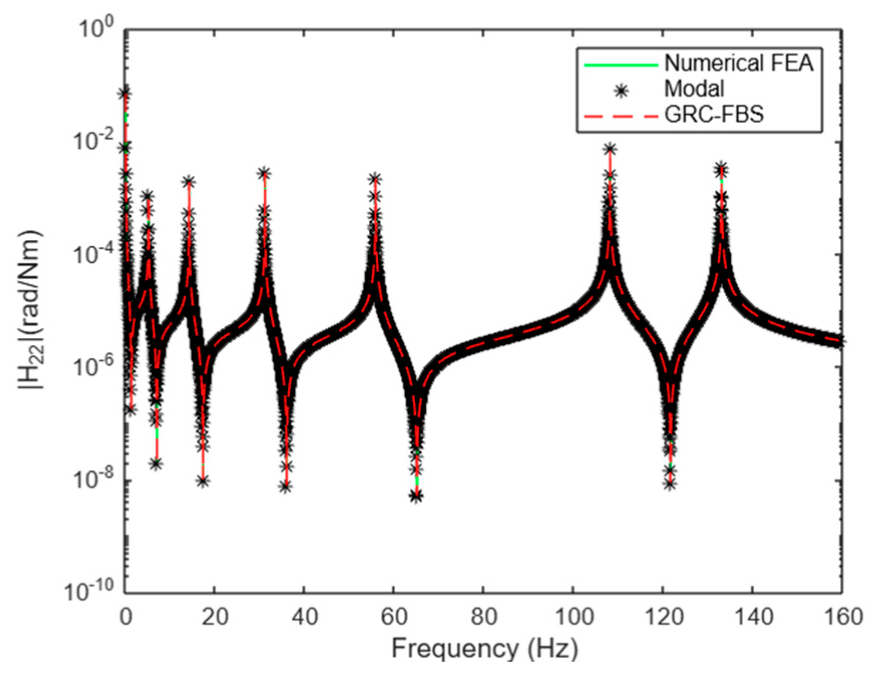
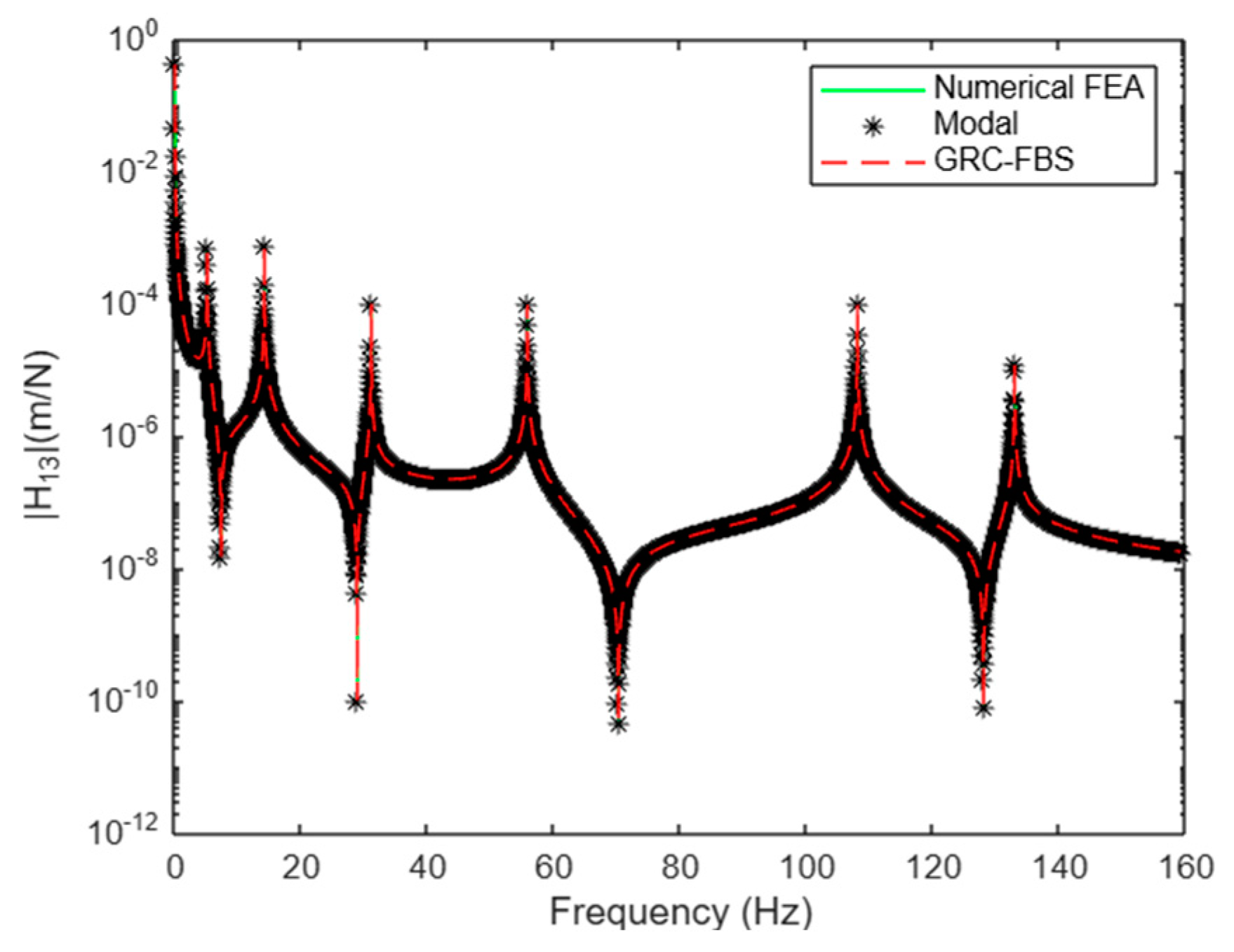
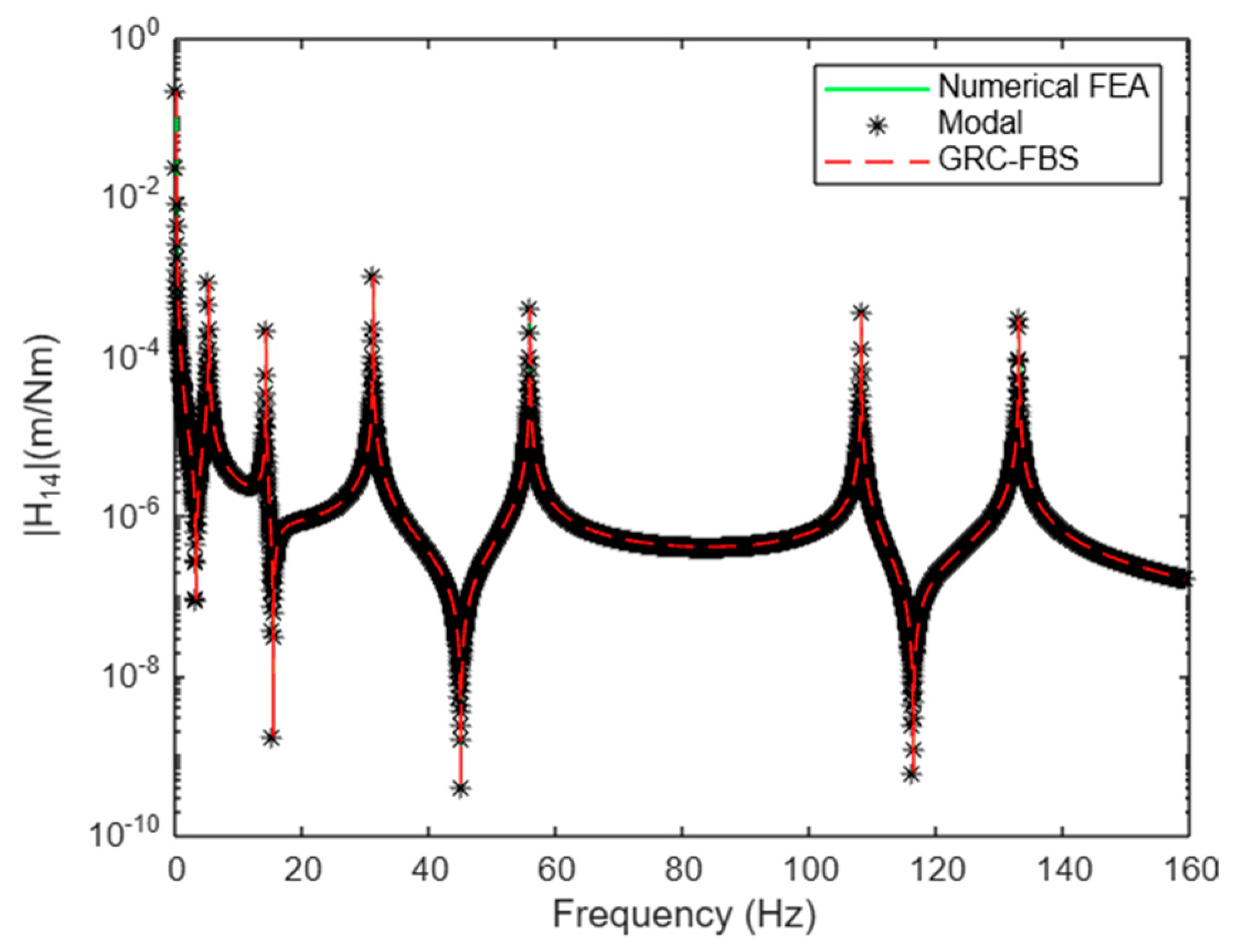
This section presents a comparative analysis of the receptance matrix components for the assembly system, derived using three different methods. The focus is on evaluating the accuracy and reliability of the GRCFBS against numerical FEA and modal analysis. The results are depicted over a frequency range covering all modes, highlighting the behavior of direct and cross receptance components. The magnitudes of the direct and cross components of the assembly system’s receptance matrix are presented in Figure 8, Figure 9, Figure 10, Figure 11, Figure 12, Figure 13, Figure 14 and Figure 15. Due to the inherent symmetry of the system, the receptance matrix components H44 and H11 exhibit similar behavior. Likewise, H33 is identical to H22 for the same reason. It compares the receptance components over a frequency range up to 160 Hz, covering all modes. Despite variations in values due to the excitation and response specifics, all three methods align well with the peaks, indicating that resonance frequencies are inherent properties of the system, independent of excitation type. The peaks observed in Figure 8, Figure 9, Figure 10, Figure 11, Figure 12, Figure 13, Figure 14 and Figure 15 correspond to the natural frequencies of the system, representing resonances where the system exhibits significant dynamic responses. Each peak signifies a mode of vibration that arises from the assembly’s structural properties, such as stiffness and mass distribution. For example, the lower-frequency peaks are generally associated with rigid body modes, where the system’s components move as a whole. Conversely, higher-frequency peaks represent flexible modes, indicating localized deformations within the structure. As summarized in Table 2 for the system ABC with eight DoFs, the lower modes (modes 1 and 2) represent rigid body motion and are observed at 0 Hz, as expected for a free–free system without constraints. The subsequent peaks correspond to flexible modes at 5.13 Hz, 14.17 Hz, 31.09 Hz, 55.81 Hz, 108.06 Hz, and 132.94 Hz. These frequencies match the dominant peaks in the receptance spectra for all components of receptance matrix, confirming that the system’s dynamic response is predominantly governed by its inherent structural properties.
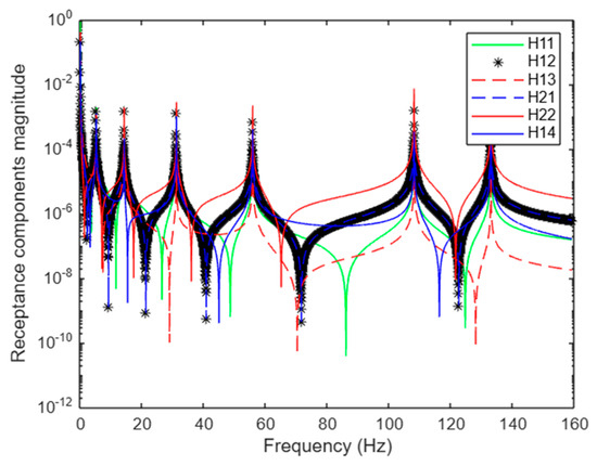
Figure 8.
Comparison between the system receptance matrix elements.
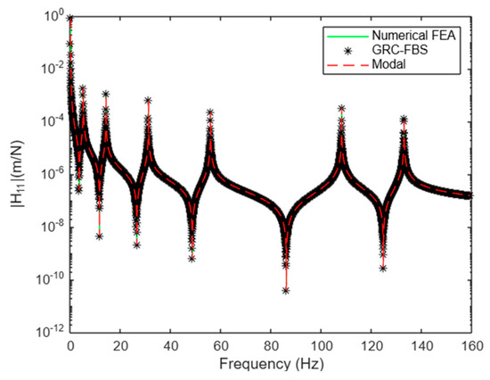
Figure 9.
Comparison of the receptance component H11 () using three different methods.
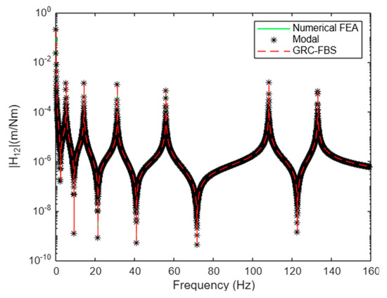
Figure 10.
Comparison of the receptance component H12 () using three different methods.

Figure 11.
Comparison of the receptance component H21 () using three different methods.
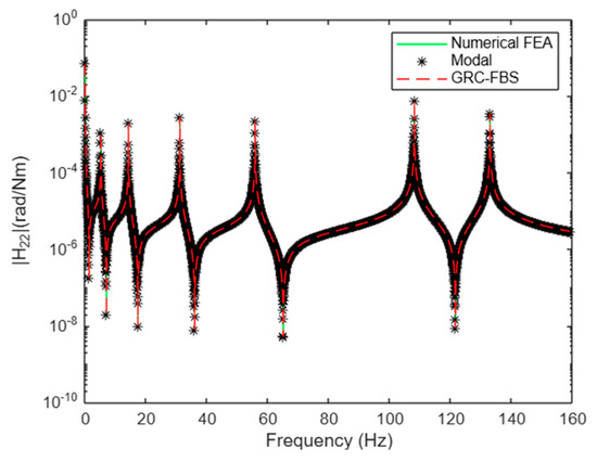
Figure 12.
Comparison of the receptance component H22 () using three different methods.

Figure 13.
Comparison of the receptance component H13 using three different methods.
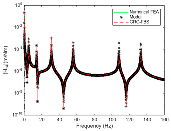
Figure 14.
Comparison of the receptance component H14 using three different methods.
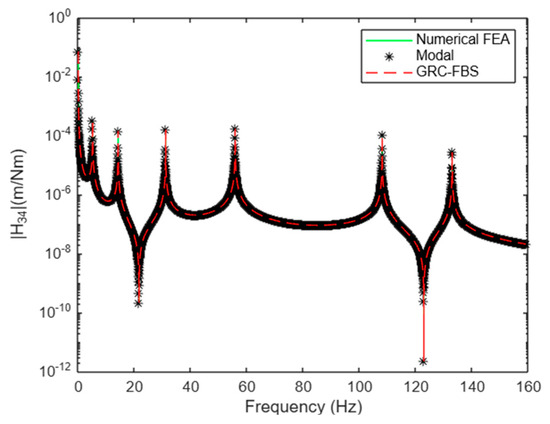
Figure 15.
Comparison of the receptance component H34 using three different methods.
The strong alignment between the predicted natural frequencies and the calculated resonance peaks from conventional methods of FEA and modal analysis validates the accuracy of the GRC-FBS method in capturing both rigid body and flexible modes.
Figure 9 compares the receptance component , representing the translational displacement at node 1 due to an excitation force applied at the same point. The results demonstrate a high degree of agreement across a frequency range covering six flexible modes.
These measurements were conducted specifically to verify the reciprocity property inherent in the system. According to this property, these components are expected to be mathematically identical, as demonstrated in the figures. represents the translational displacement at node 1 resulting from an excitation couple applied at the same point, while represents the angular displacement at node 1 resulting from an excitation force applied at the same point. The identical appearance of the graphs serves as confirmation of the reciprocity property, validating the theoretical approach. This verification is critical for ensuring the robustness of the methodology across the frequency range.
Figure 12 compares the receptance component , representing the rotational displacement at node 1 due to an excitation couple applied at the same point, and shows a strong alignment with the numerical FEA and modal analysis, verifying the effectiveness of the generalized coupling method. The resonant peaks corresponding to the flexible modes are accurately depicted by the GRC-FBS method, with natural frequencies deriving from the other two methods. It is worth noting that rigid body modes have also been predicted by this method in addition to natural frequencies corresponding to flexible modes.
Figure 13 compares the receptance component , describing the translational displacement at node 1 due to an excitation force applied at point 2, across three methods, showing a strong alignment at low frequencies, where it represents the translational displacement at node 1 due to a force at point 2. Figure 14 and Figure 15 similarly compare and , representing translational displacements at nodes 1 and 2 due to couples at node 2. These figures demonstrate a strong correlation in undamped systems at low frequencies. However, deviations are expected at higher frequencies and in damped systems with complex geometries due to increased modeling challenges. Figure 13, Figure 14 and Figure 15 demonstrate the effect of cross-coupling between substructures. However, it is important to note that for higher-frequency ranges and in damped systems with more complex geometries, deviations between the methods are inevitable. These deviations may be attributed to the increased complexity and the challenges associated with accurately modeling the dynamic interactions at higher frequencies.
The close alignment of results across the three methods is expected due to the use of three rigidly coupled beam elements without damping, where the receptance of substructures is derived from the beam element’s mass and stiffness matrices. Additionally, the analysis focuses on low-frequency ranges, where such methods typically yield consistent results due to the simplified dynamic behavior of the system. This comparison demonstrates the validity and reliability of the generalized coupling method for predicting the dynamic structure responses composed of multiple substructures.
6. Limitations
The Frequency-Based Substructuring (FBS) method, multi-body dynamic (MBD) modeling, and finite element analysis (FEA) offer distinct advantages depending on the system and objectives of analysis. The FBS approach reduces the complexity of dynamic systems by operating in the frequency domain, making it efficient for systems with small deformations and linear behavior. It simplifies the analysis by coupling subsystems’ FRFs, enabling hybrid modeling with computational efficiency. However, FBS is not suitable for systems involving large motions or significant non-linearities due to its reliance on linear superposition principles. MBD methods, on the other hand, are designed for analyzing non-linear dynamics, large motions, and contact mechanics in the time domain. While MBD is a versatile technique, its simulations are computationally intensive and highly sensitive to time-step sizes. FEA provides detailed spatial resolutions of system behavior and is widely used for static and dynamic structural analysis. Unlike FBS, which focuses on system decomposition, and MBD, which emphasizes motion dynamics, FEA excels in capturing localized stress and strain but can become computationally expensive for large-scale or highly dynamic systems due to its reliance on extensive datasets. Together, these methods complement each other, with FBS offering efficiency for reduced-order modeling and predicting system responses—particularly in the early stages of development when the entire system is not available, but subsystems’ receptances or FRFs can be measured and utilized effectively.
While the proposed methodology is highly effective for linear and lightly non-linear systems, it faces challenges in handling highly non-linear systems or complex damping scenarios. The framework excels in systems exhibiting mild non-linearities, where response predictions can be relatively standardized. However, as non-linear interactions such as hysteresis, complex phase damping, or highly non-linear joints become significant, the GRCFBS approach’s applicability is not valid because the diverse nature of non-linear interactions and interfaces makes standardization difficult. The accuracy of the results is also highly dependent on the quality of measured FRFs in the experimental approach, with noise and non-linearities at interface connections posing additional challenges. Future developments could address these limitations by incorporating advanced non-linear substructuring techniques or leveraging machine learning to predict and correct non-linear behaviors. Moreover, the framework is most efficient for modular, reconfigurable systems, where substructuring assumptions are true. As non-linear behaviors grow more complex across subsystems, more sophisticated methods will be required to maintain prediction accuracy.
In systems with significant non-linearities, the methodology using substructuring technique relies on approximations, such as linearizing non-linear joints or representing local non-linear dynamics as additional dynamic stiffness. These can be incorporated as “black-box” subsystems using experimental receptance measurements at critical points. Current research efforts aim to develop algorithms capable of integrating complex non-linear dynamics into substructuring techniques, but such advancements are still under development.
7. Conclusions
This paper introduces an efficient approach for modeling reconfigurable dynamic systems applicable across diverse fields such as robotics, aerospace, and manufacturing. The methodology incorporates two generalized receptance coupling methods: Jetmundsen and D.D. Klerk’s FBS-based approach, both providing a pragmatic framework for modeling linear dynamic systems with complex configurations. The strength of receptance coupling lies in its efficiency and simplicity, focusing only on critical DoFs at coupling locations and key measurement points. This selective approach significantly reduces the model’s complexity by concentrating on the most relevant aspects, making it particularly valuable in the early stages of development when data are scarce for the target setting and target cascading of noise and vibration attributes.
A key feature of this methodology is its ability to facilitate reduced-order modeling. By focusing on essential DoFs and key system components, the approach enables the creation of simplified yet accurate models, which are crucial for efficient simulation and analysis, especially in systems with complex dynamics. This reduction in model complexity not only accelerates computational processes but also enhances the practicality of the method in iterative design phases.
This methodology also facilitates the development of a hybrid model capable of predicting system responses based on receptance matrices measured from disassembled subsystems or components, which are easier to measure. Unlike traditional NVH methods that rely heavily on the availability of subsystem data, this proactive approach proves effective in early development phases, reducing costs and design time. The use of direct FRFs, obtained either through measurement or numerical simulation, offers lower potential error rates compared to traditional techniques like modal coupling, which suffer from mode truncation impacting system properties such as stiffness and mass, especially in the high-frequency range.
While the direct inversion of non-square matrices may be infeasible, pseudo-inverse matrices are crucial in coupling methods, enabling the analysis of interconnected subsystems with different DoFs. Although this approach does not depend on whether substructures’ receptance matrices are derived from experimental measurements or theoretical calculations, noisy measured data should be filtered using regularization techniques like Singular Value Decomposition (SVD) to obtain robust solutions.
The first analytical case study demonstrated that both the Jetmundsen and LM FBS algorithms yield similar results, further validating the approach. The comparison of the GRC-FBS method with numerical FEA and modal methods in the second case study confirms the proposed method’s accuracy, as evidenced by the alignment of resonance peaks and the pattern of change in receptance components with frequency. The strong agreement between these methods underscores the effectiveness and accuracy of the approach. However, the simplicity of the numerical case study—assuming rigid couplings, a single element, and an undamped system—was intentionally chosen to clearly illustrate the methodology, its accuracy, and its potential applications for more complex systems. For higher-frequency regions, inevitable shifts in resonance and anti-resonance peaks may occur due to the assumptions used in the development of the methodology. However, the limitations of modal analysis, particularly in complex systems where mode truncation can distort system properties and lead to errors, are not present in this method.
It is noteworthy that the findings and methodology described here have significant potential for expansion into real-world scenarios, which could drive new developments in the field, particularly in the dynamics of structures and vibration analysis.
Author Contributions
Conceptualization, B.H. and S.T.; methodology, B.H.; software, B.H.; validation, B.H. and S.T.; formal analysis, B.H.; investigation, B.H.; resources, S.T.; data curation, B.H.; writing—original draft preparation, B.H.; writing—review and editing, B.H.; visualization, S.T.; supervision, S.T.; project administration and funding acquisition, S.T. All authors have read and agreed to the published version of the manuscript.
Funding
This research received no external funding.
Data Availability Statement
The data presented in this study, including the detailed design of the double damper, are available on request from S.T. The technical data are not publicly available due to confidentiality.
Acknowledgments
I would like to express my sincere appreciation to Saied Taheri, in CenTiRe at Virginia Tech, for his invaluable guidance and support throughout this work. I am also grateful to the Engineering Mechanics program at Virginia Tech for providing me the opportunity to be involved in this research.
Conflicts of Interest
The authors declare no conflicts of interest.
References
- Astrid, P.; Weiland, S.; Willcox, K.; Backx, T. Missing point estimation in models described by proper orthogonal decomposition. In Proceedings of the 2004 43rd IEEE Conference on Decision and Control (CDC) (IEEE Cat. No.04CH37601), Nassau, Bahamas, 14–17 December 2004. [Google Scholar] [CrossRef]
- Bishop, R.E.D.; Johnson, D.C. The Mechanics of Vibration; Cambridge University Press: Cambridge, UK, 1960. [Google Scholar]
- O’Hara, G.J. Advances in structural dynamics: Analysis of complex mechanical structures. ASME J. Appl. Mech. 1976, 43, 292–298. [Google Scholar]
- Ewins, D.J.; Gleeson, J.G. Identification of modal properties using frequency response functions. J. Sound Vib. 1985, 104, 289–308. [Google Scholar]
- Jetmundsen, R. Generalized receptance coupling and modal synthesis. J. Sound Vib. 1988, 124, 131–146. [Google Scholar]
- De Klerk, D.; Rixen, D.J.; De Jong, J. The frequency-based substructuring method as a basis for component mode synthesis. J. Sound Vib. 2006, 308, 303–329. [Google Scholar]
- Zhang, W.; Song, L.; Xu, J. Dynamic behavior analysis of subframe-body assembly using frequency-based substructuring. Mech. Syst. Signal Process. 2017, 92, 290–306. [Google Scholar]
- Kang, S.; Choi, Y.; Kim, S. Inverse substructuring for road noise reduction in suspension systems. SAE Int. J. Passeng. Cars–Mech. Syst. 2019, 12, 123–132. [Google Scholar]
- Wagner, P.; Hülsmann, T.; Van der Seijs, W.; BMW Group. Application of dynamic substructuring for NVH analysis in electric drivetrains. Int. J. Automot. Eng. 2020, 11, 250–265. [Google Scholar]
- Tsai, H.C. Extension of rotational receptance measurement techniques for improved dynamic substructuring. J. Vib. Control 2019, 25, 478–495. [Google Scholar]
- Clontz, M.; Taheri, S. Decoupling of tire and suspension subsystems using frequency-based substructuring. Veh. Syst. Dyn. 2017, 55, 1120–1138. [Google Scholar]
- Voormeeren, S.N.; Rixen, D.J. Uncertainty quantification in frequency-based substructuring: The effect on dynamic response prediction. J. Sound Vib. 2022, 527, 116767. [Google Scholar]
- De Klerk, D.; Rixen, D.J.; De Jong, J. Advanced algorithms for subsystem coupling in frequency-based substructuring. Mech. Syst. Signal Process. 2021, 151, 107368. [Google Scholar]
- De Klerk, D.; Rixen, D.; Voormeeren, S.N. General framework for dynamic substructuring: History, review, and classification of techniques. AIAA J. 2008, 46, 1169–1181. [Google Scholar] [CrossRef]
- Liu, Y.; Mir, S. Hybrid method for vehicle axle noise simulation with experimental validation. J. Vib. Acoust. 2003, 125, 496–504. [Google Scholar]
- Li, J.; Sun, Z.; Zhou, Z. Application of dynamic substructuring in railway vehicle dynamics. J. Rail Rapid Transit 2021, 235, 450–462. [Google Scholar]
- Scheel, T.; Sturzenegger, M. Application of frequency-based substructuring in satellite dynamic analysis. Aerosp. Sci. Technol. 2020, 104, 106294. [Google Scholar]
- Nguyen, H.Q.; Lee, H.; Park, J.H. Modular robotic system dynamics using frequency-based substructuring. Robot. Auton. Syst. 2022, 140, 103788. [Google Scholar]
- Gebhardt, C.; Müller, P.; Wingerde, A.M. Dynamic analysis of wind turbine blades using frequency-based substructuring. Wind Energy 2020, 23, 1934–1950. [Google Scholar]
- Park, K.H.; Jung, S.; Lee, Y.S. Marine vessel hull vibration analysis using frequency-based substructuring. J. Mar. Sci. Eng. 2023, 11, 412. [Google Scholar]
- Lee, S.; Kim, J.; Lee, J.H. Frequency-based substructuring for dynamic analysis of civil structures. Eng. Struct. 2021, 239, 112280. [Google Scholar]
- El Mahmoudi, A.; Paracha, U.S.; Rixen, D. Design optimization of joint parameters using Frequency Based Substructuring. PAMM 2019, 19, e201900454. [Google Scholar] [CrossRef]
- Kang, Y.J.; Kim, J.G.; Song, D.P.; Ih, K.D. Derivation of road noise improvement factor within a suspension system using the inverse substructuring method. Proc. Inst. Mech. Eng. Part D J. Automob. Eng. 2019, 233, 2492–2501. [Google Scholar] [CrossRef]
- Schmitz, T.; Cornelius, A.; Karandikar, J.; Tyler, C.; Smith, S. Receptance coupling substructure analysis and chatter frequency-informed machine learning for milling stability. CIRP Ann. 2022, 71, 445–448. [Google Scholar] [CrossRef]
- Albertelli, P.; Goletti, M.; Monno, M. An Improved Receptance Coupling Substructure Analysis to Predict Chatter-Free High-Speed Cutting Conditions. Procedia CIRP 2013, 12, 19–24. [Google Scholar] [CrossRef]
- Hamedi, B.; Taheri, S. Fundamental Review of Hybrid and Modular Modeling Approaches for Road Noise Prediction: Insights from a Fundamental Quarter Car Model. Univers. J. Mech. Eng. 2024, 12, 25–35. [Google Scholar] [CrossRef]
- Hamedi, B.; Taheri, S. Reduced-Order Modeling for Dynamic System Identification with Lumped and Distributed Parameters via Receptance Coupling Using Frequency-Based Substructuring (FBS). Appl. Sci. 2024, 14, 9550. [Google Scholar] [CrossRef]
- Hamedi, B.; Taheri, S. Modular Modeling of a Half-Vehicle System Using Generalized Receptance Coupling and Frequency-Based Substructuring (GRCFBS). Vibration 2024, 7, 1063–1085. [Google Scholar] [CrossRef]
- Jetmundsen, B.; Bielawa, R.L.; Flannelly, W.G. Generalized frequency domain substructure synthesis. J. Am. Helicopter Soc. 1988, 33, 55–64. [Google Scholar] [CrossRef]
- Thulasiraman, K.; Swamy, M.N.S. Graphs: Theory and Algorithms; John Wiley & Sons: Hoboken, NJ, USA, 1992; ISBN 9780471513568. [Google Scholar] [CrossRef]
- Clontz, M. A Novel Method for Vibration Analysis of the Tire-Vehicle System via Frequency-Based Substructuring. Ph.D. Thesis, Virginia Polytechnic Institute and State University, Blacksburg, VA, USA, May 2018. [Google Scholar]
- TurboSquid. Tesla Model S Chassis 2. Available online: https://www.turbosquid.com/3d-models/tesla-s-chassis-2-3d-max/983582 (accessed on 26 November 2024).
- Bathe, K.J. Finite Element Procedures; Prentice Hall: Upper Saddle River, NJ, USA, 2006. [Google Scholar]
- Zienkiewicz, O.C.; Taylor, R.L. The Finite Element Method. In The Basis; Butterworth-Heinemann: Oxford, UK, 2000; Volume 1. [Google Scholar]
- Ewins, D. Modal Testing: Theory and Practice; Wiley: New York, NY, USA, 1985. [Google Scholar]
- Luo, F.; Hu, X.; Zhang, D. A regularization method for ill-conditioned problems with applications in FRF-based substructuring analysis. J. Vib. Control 2020, 26, 1321–1330. [Google Scholar]
- Zheng, Y.; Lin, L.; Zhang, Y. A study on the ill-conditioned problem of inverse force identification using pseudo-inverse method with Tikhonov regularization. Mech. Syst. Signal Process. 2019, 120, 615–634. [Google Scholar]
- Golub, G.H.; Van Loan, C.F. Matrix Computations, 4th ed.; Johns Hopkins University Press: Baltimore, MD, USA, 2013. [Google Scholar]
- Zhou, X.; Ma, S.; Zhang, H.; Fang, W. Enhanced SVD-based method for noise reduction in experimental modal analysis. J. Sound Vib. 2023, 548, 117607. [Google Scholar]
- Qin, L.; Yang, L.; Ji, T. A regularization method for ill-conditioned problems in inverse structural dynamics. Mech. Syst. Signal Process. 2021, 151, 107368. [Google Scholar]
- Chen, Z.; Chan, T.H.T. A truncated generalized singular value decomposition algorithm for moving force identification with ill-posed problems. J. Sound Vib. 2017, 401, 297–310. [Google Scholar] [CrossRef]
Disclaimer/Publisher’s Note: The statements, opinions and data contained in all publications are solely those of the individual author(s) and contributor(s) and not of MDPI and/or the editor(s). MDPI and/or the editor(s) disclaim responsibility for any injury to people or property resulting from any ideas, methods, instructions or products referred to in the content. |
© 2024 by the authors. Licensee MDPI, Basel, Switzerland. This article is an open access article distributed under the terms and conditions of the Creative Commons Attribution (CC BY) license (https://creativecommons.org/licenses/by/4.0/).

