Causes of Multi-Mechanism Abnormal Formation Pressure in Offshore Oil and Gas Wells

Abstract

This study thoroughly investigates the complex origins of abnormal formation pressure in offshore oil and gas wells, taking the Rio del Rey Basin in Cameroon as a case study. Renowned for its abundant oil and gas resources, the area faces unique challenges in predicting overpressure due to its high-temperature and high-pressure reservoir characteristics. By quantitatively analyzing the main mechanisms such as undercompaction, high-temperature fluid expansion, and mud diapirism, the study addresses the complexities of overpressure prediction. This paper introduces an innovative analytical framework that combines hierarchical clustering algorithms with the LightGBM model. Further refined by the application of Bayesian optimization, the model intelligently adjusts hyperparameters to enhance predictive accuracy. Utilizing well logging data and applying machine learning techniques, the paper classifies and identifies different mechanisms causing abnormal pressures, achieving a model prediction accuracy of 0.942. The research findings highlight the predominant role of the undercompaction mechanism, accounting for approximately 70% of the abnormal high-pressure events in the study area. Fluid expansion and shale diapirism contribute smaller but significant proportions of 10% and 20%, respectively. These quantitative insights into the pressure mechanisms are vital for optimizing drilling operations and reducing risks in oil and gas exploration. The study’s hybrid approach, integrating geophysical analysis with advanced computational techniques, sets a precedent for future research. It provides new avenues for applying machine learning to understand complex geological phenomena in similar geological environments and makes a significant contribution to the strategic planning of hydrocarbon exploration and production activities.

1. Introduction

The Rio del Rey Basin in Cameroon is located on the northeastern edge of the Niger Delta Basin and is rich in oil and gas resources, making it the primary oil-producing region in Cameroon. The deep turbidite sand bodies within this block represent the next targets for exploration and production. These deep turbidite sandstone reservoirs are buried at depths ranging from 2500 to 3500 m, with a maximum formation pressure coefficient of 2.10, the highest bottom-hole temperature reaching 161 °C, and a maximum geothermal gradient of 4.6 °C/100 m, classifying them as typical high-temperature and high-pressure reservoirs. These reservoirs are relatively young in terms of diagenesis and are influenced by fault blocks and mud diapirism. The causes of overpressure are complex, potentially influenced by the undercompaction of strata, high-temperature fluid expansion, mud diapirism, and fault block development, leading to a multifaceted pressure system. Conventional prediction methods based on sediment compaction theory primarily apply to the undercompaction mechanism of sandstone and mudstone strata, while the Bowers unloading model is predominantly used for fluid expansion strata [1]. However, for the multi-mechanism superposition observed in this area, single-pressure mechanism prediction methods can yield significant errors and fail to provide precise predictions. Since the 1990s, the importance of accurately determining the pressure mechanism has been increasingly recognized. Early studies primarily relied on qualitative inferences related to sedimentary evolution, stratigraphic mineral composition, and hydrocarbon migration characteristics; however, these methods often lack substantial data support and can vary greatly depending on the individual researcher’s understanding of the geological context. In later studies, the incorporation of well logging data and rock mechanics has led to more intuitive and convincing judgments [2]. For instance, Teige [3] summarized well logging data from a Norwegian field, noting that low acoustic velocity and resistivity, without distinct abnormal high-pressure sections in porosity and density curves, are likely indicative of fluid expansion. Bowers [4] introduced the acoustic-density crossover method to discern the causes of undercompaction, pore fluid expansion, and tectonic compression by analyzing the positional relationships between measured data points and the ideal loading curve. Nevertheless, this method has limitations in identifying subtle causes such as diapirism. Ye et al. [5] proposed a method to distinguish between undercompaction and tectonic compression mechanisms, considering specific regional structures and sedimentation. Although the processes of undercompaction and tectonic compression share similarities, they fundamentally differ; undercompaction typically involves a one-dimensional perspective where vertical stress from sediment loading leads to abnormal pressure due to incomplete dewatering, while tectonic compression operates in three dimensions, with horizontal and vertical stresses interacting due to tectonic forces such as faulting or folding. Ye et al. [5] pointed out that in areas where the folds are not tight, high-stress tectonic compression generally does not occur; however, near mountain fronts and active large reverse faults, tectonic compression can be significant. The acoustic emission test of underground coring can thus be used to determine the magnitude of in situ stress. Building on this line of reasoning, Zhang et al. [6] added the factor of overpressure transmission and proposed an identification pattern diagram based on these four mechanisms, which can distinguish between unbalanced compaction and tectonic compression; however, they noted difficulties in estimating fluid expansion and overpressure transmission. In 2017, Fan et al. emphasized that when acoustic density and resistivity logging curves are plotted on the same depth coordinate system, significant deviations in all three curves at the same logging depth confirm the occurrence of undercompaction [7]. Recently, Guo et al. [8] utilized a multi-well logging curve combination method and Bowers’ acoustic density crossover diagram to identify the causes of overpressure in the Yinggehai Basin, highlighting the relevance of advanced logging techniques in pressure assessment. Furthermore, Ai et al. [9] combined mud mineral analysis with acoustic time difference-density crossover diagram analysis to determine different compaction stages, yielding ideal predicted pressure results. This showcases the application of innovative methodologies in addressing traditional overpressure assessment challenges.

In addition, recent advances in machine learning and artificial intelligence have shown great promise in predicting abnormal pressure conditions. For instance, Chen et al. [10] explored the use of support vector machines and neural networks for predicting pore pressure in complex geological environments, demonstrating improved accuracy and reliability over traditional methods. Similarly, Liu et al. [11] applied deep learning techniques to analyze logging data, revealing patterns in abnormal pressure occurrences that were previously undetectable through conventional approaches. The primary objective of this study is to provide a robust framework for quantifying traditional overpressure mechanisms in the Rio del Rey Basin. We employ a comprehensive approach that integrates theoretical judgment with hierarchical clustering algorithms to calculate the weights associated with different causes of overpressure. By utilizing a powerful LightGBM model enhanced with the SMOTE Bayesian optimization algorithm, we have developed an effective model for identifying the mechanisms responsible for abnormal pressure. This method not only enables the calculation of formation pressure applicable to the combined effects of undercompaction, high-temperature fluid expansion, and structural diapirism but also provides a scientific basis for subsequent oil and gas exploration. By gaining a deeper understanding and quantifying these abnormal pressure mechanisms, this research will offer important support for optimizing drilling and production decisions, thereby reducing operational risks and enhancing the efficiency and safety of resource extraction. The findings of this study not only enrich the theoretical framework of overpressure mechanisms but also provide new ideas and methods for research in similar geological environments, holding significant practical implications for the oil and gas industry.

2. Mechanisms of Abnormal Formation Pressure

Abnormal formation pressure or abnormal formation pore pressure primarily includes abnormally low pressure and abnormally high pressure, both of which are widely present in major oil and gas basins around the world. Among these, abnormally high pressure is more common, while abnormally low pressure is relatively rare. The mechanisms behind abnormally high pressure are highly complex and can be triggered by a single factor or by the combined effect of multiple factors. Geological deposition, chemical reactions, and physical processes can all contribute to an abnormal increase in underground fluid pressure. Common causes of abnormally high pressure include undercompaction, hydrocarbon generation from source rock cracking, tectonic compression, fault activity, and diapirism. Undercompaction occurs when sediment layers fail to consolidate adequately due to rapid sedimentation, leading to an increase in pore pressure [6]. Hydrocarbon generation involves the thermal cracking of organic matter in source rocks, which can produce additional fluid and increase pore pressure [12]. Tectonic compression arises from the interaction of tectonic plates and can significantly alter stress conditions in the subsurface [8]. Fault activity can create pathways for fluid migration, resulting in localized pressure increases [1]. Diapirism, characterized by the upward movement of less dense materials, can also impact fluid dynamics and pressure distributions [9]. These factors often interact, leading to even more complex pressure systems. For instance, Zhang et al. [6] demonstrated that undercompaction and tectonic forces can coexist, complicating the pressure profiles in sedimentary basins. To better understand these interactions, Fan et al. [13] classified the causes of abnormally high pressure into four categories based on changes in vertical effective stress during sedimentary loading. These categories include:

1.

Primary Sedimentary Loading Mechanism—Undercompaction

During diagenesis, as sediments accumulate, pressure from the overlying rock layers increases, continuously squeezing water out of the sediments. As a result, vertical effective stress increases and porosity decreases with the enhanced compaction. The normal compaction process involves an increase in vertical effective stress, i.e., continuous loading. Undercompaction occurs when water in the sediments cannot be expelled smoothly, resulting in porosity that does not decrease with increased compaction. Vertical effective stress either slows its rate of increase or remains unchanged, while the overlying rock pressure continues to increase normally. According to effective stress theory, this leads to the occurrence of abnormally high pressure [14,15,16].

2.

Reloading Mechanism—Tectonic Activity

Under certain conditions, tectonic activity can close open fractures, making it difficult for fluids to be expelled, reducing porosity while the overlying rock pressure remains unchanged. As vertical effective stress decreases, abnormally high pressure naturally occurs according to rock effective stress theory. Common tectonic compression involves the distribution of stress between rock volume and fluids, including rock porosity, rock and fluid compressibility properties, and rock stress in sedimentary basins. Stress can only be converted into pore fluid pressure when fluid flow is restricted (tectonic compression can locally open fluid channels, leading to abnormally low pressure). Similar effects are seen with diapirism, fault activity, and salt domes, provided that fluid channels can be closed. Since fault activity can sometimes connect fluid pathways, geological conditions must be carefully considered when dealing with such abnormal high pressures [17,18,19,20].

3.

Unloading Mechanism—Pore Fluid Expansion

During or after compaction, pore fluid volume increases or the overlying rock pressure decreases due to one or more reasons, reducing vertical effective stress.

a.

Hydrocarbon Generation and Thermal Cracking of Hydrocarbons

Hydrocarbon generation: Kerogen in source rock transforms into less dense oil and gas, causing pore fluid volume to expand. After hydrocarbon expulsion, the fluid migrates to the reservoir, with the pore fluid bearing part of the overlying rock load, resulting in abnormally high pressure.

b.

Transformation from Montmorillonite to Illite

Montmorillonite is a very common clastic mineral found in shale, and its crystal structure contains abundant interlayer water. When montmorillonite is freshly deposited, it undergoes hydration. This hydration process continuously absorbs free water between the crystal particles, increasing the fluid volume in the pores.

c.

Transformation from Gypsum to Anhydrite

The transformation from gypsum to anhydrite releases crystallization water, while anhydrite absorbs water and converts back to gypsum. This process causes anhydrite to absorb water and expand, increasing rock volume and reducing rock porosity, which can also lead to higher pressure.

4.

Minimal Change in Porosity

Although the porosity remains essentially unchanged, abnormal high pressure can still occur. For example, mineral transformations (such as the conversion of montmorillonite to illite) may lead to the redistribution of fluids and an increase in pressure, even though there is little change in porosity. Additionally, chemical reactions between fluids can result in the generation of dissolved gases or minerals, thereby increasing the pressure of the pore fluids. For instance, reactions between groundwater and dissolved carbonate minerals can lead to the formation of gas bubbles, which causes fluid pressure to rise. These mechanisms are crucial for understanding the complexity of subsurface pressures and their implications for oil and gas exploration [21,22].

2.1. Data Collection for the Target Work Area

(1)

Basic Data

Comprehensive and accurate input data can reflect the overall characteristics of a block and assist researchers in analyzing specific wells. The input data collected in this study primarily include the stratigraphy of the Rio del Rey Basin in Cameroon, a comprehensive geological logging database for key wells, drilling fluid usage, drill bit usage, and records of drilling complexities.

(2)

Logging Data

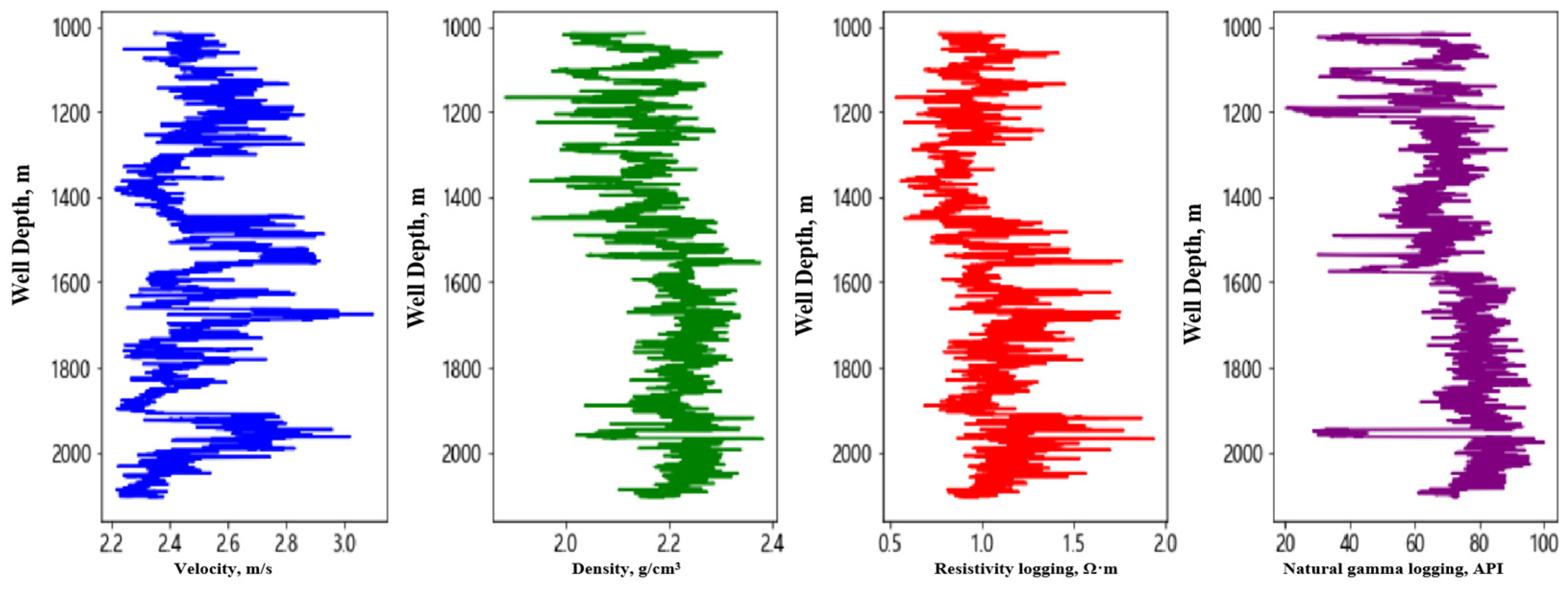
The conventional method for calculating formation pore pressure using logging data involves calculating effective stress, using sonic time delay data, and the overlying formation pressure, using density logging data. The pore pressure is then determined by combining these values through effective stress theory. Two main factors influence the reliability of formation pressure calculations: ① the quality of logging data and the preprocessing methods used, and ② the model used to derive the formation pore pressure. Therefore, it is important to use high-quality sonic time delay logging data (generally with a clear mudstone trend and minimal borehole enlargement) and available density logging data, with sufficiently long logging intervals. Additionally, it is crucial to eliminate interference factors and false data points as much as possible. By preliminarily processing the original sonic time delay and density data, it is possible to obtain relatively pure mudstone sonic time delay and mud density data, which are closer to the true formation conditions. Based on this, a pore pressure calculation model that matches the actual regional conditions can be selected to achieve ideal detection results. In the studied block, collected logging data include well depth, sonic time delay, natural gamma, P wave velocity, porosity, shale content, density, and overlying formation pressure [23,24,25].

(3)

Seismic Data

Two-dimensional seismic data inversion requires seismic line data and individual well logging data. Preferably, seismic lines that pass through wells or are adjacent to wells (if no lines directly pass through wells) should be used. Post-stack migration pure wave seismic data and corresponding wells should be selected, with priority given to two cross-lines that intersect at wells and their corresponding wells, lines passing through multiple wells, or lines near many wells. The selected lines should reflect the research area’s spatial arrangement. Corresponding interpreted horizon data, geological layering, and time–depth conversion data (VSP, geological layering data such as boundary depths, formation codes, or names) should also be used [26,27,28].

2.2. Data Sorting and Analysis

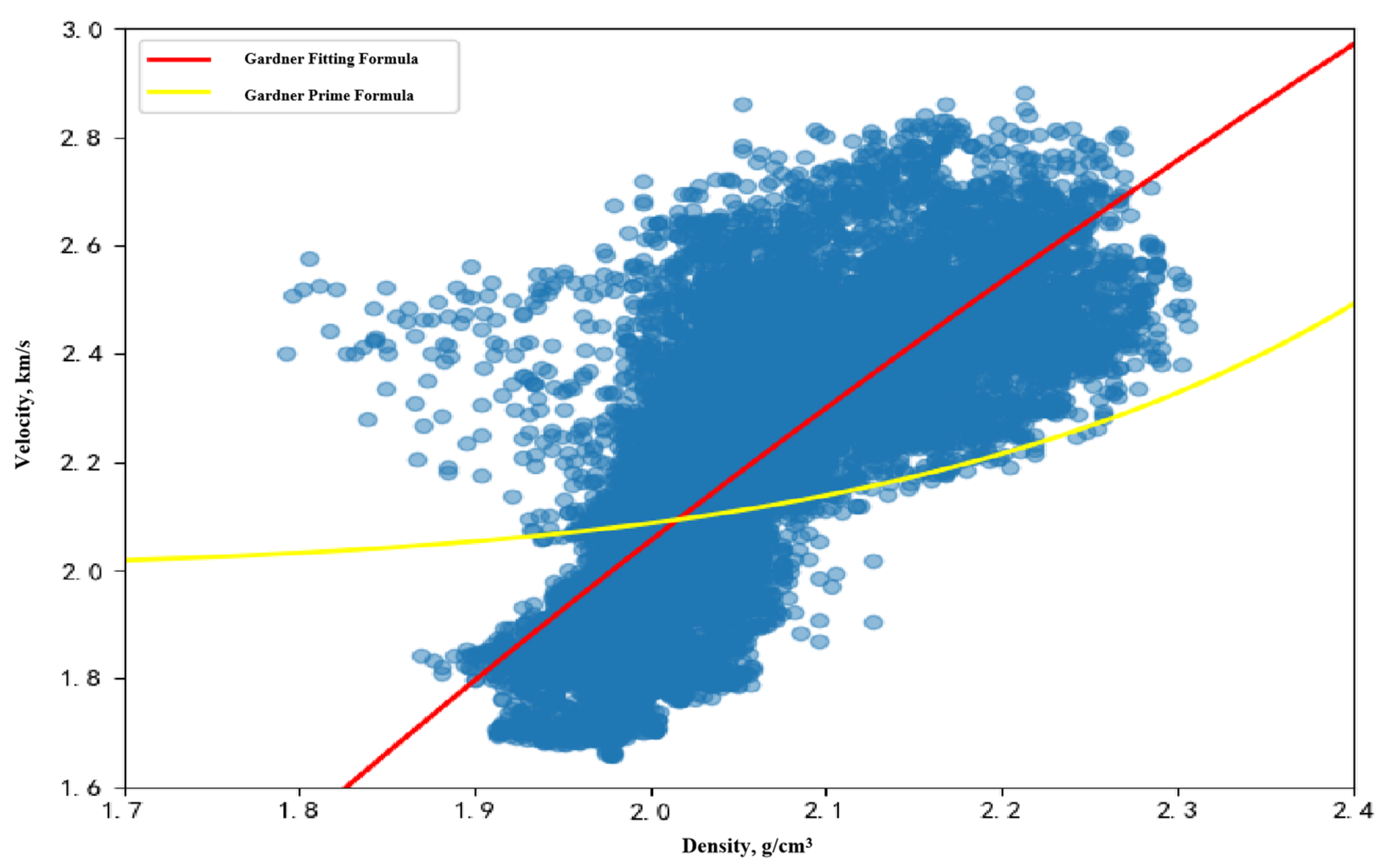
Based on the collected logging data, this study extracted and organized P wave velocity and density data at equivalent depths in the block, presenting them in a velocity–density cross-plot. The cross-plot shows the relationship between P wave velocity and density over the entire well depth, with each data point corresponding to specific values at certain depths. Detailed analysis of the cross-plot can extract important information about formation properties, especially the mechanisms behind abnormal formation pressures. In the plot, normal formations typically exhibit a linear trend representing the relationship between porosity and mineral composition. However, any anomalies deviating from this trend may indicate abnormal formations. The velocity–density cross-plot’s variations over the entire well depth are shown in Figure 1.

From the P wave velocity and density cross-plot, three main mechanisms for abnormal pressure can be identified: undercompaction, fluid expansion, and mudstone diapirism.

(1)

Undercompaction: Rapid sedimentation may not allow for proper compaction, resulting in higher porosity and lower density. P wave velocity and resistivity can reflect porosity to some extent; thus, lower velocity and higher resistivity may indicate undercompaction. This corresponds to the lower value area along the normal trend line in the velocity–density cross-plot.

(2)

Tectonic Compression: Additional compaction beyond that due to the sedimentary one lead to overcompaction, where pores are compressed and fractures are closed, resulting in increased P wave velocity (reduced resistivity, decreased porosity), though density increases only slightly. Mudstone diapirism, differs in the direction of compression compared to expected tectonic offset and transport. This corresponds to the higher value area along the normal trend line in the velocity–density cross-plot, similar to an inverse unloading line.

(3)

Fluid Expansion: Including hydrothermal pressurization and hydrocarbon generation (oil and gas). On the basis of normal sedimentary compaction, the rock volume is expanded by fluids, reducing P wave velocity (increasing resistivity), though density changes slightly. The temperature relative to the normal geothermal gradient is higher. Pressure changes caused by hydrothermal pressurization can be quantified by the thermal expansion coefficient of water. Structural compression can be seen as overloading, while fluid expansion as unloading. This corresponds to the lower velocity value area along the normal trend line in the velocity–density cross-plot, positioned on the unloading line.

In the studied area’s velocity–density cross-plot, actual data for high-pressure anomalies show distinct characteristics. Specifically, undercompaction occupies a larger proportion throughout the area, concentrated in shallower and mid-level formations. Further analysis indicates fluid expansion phenomena are mainly in mid-level and deeper formations, while mudstone diapirism is primarily found to occur in deep formations.

3. Methods for Determining Causes of Abnormal Formation Pressure

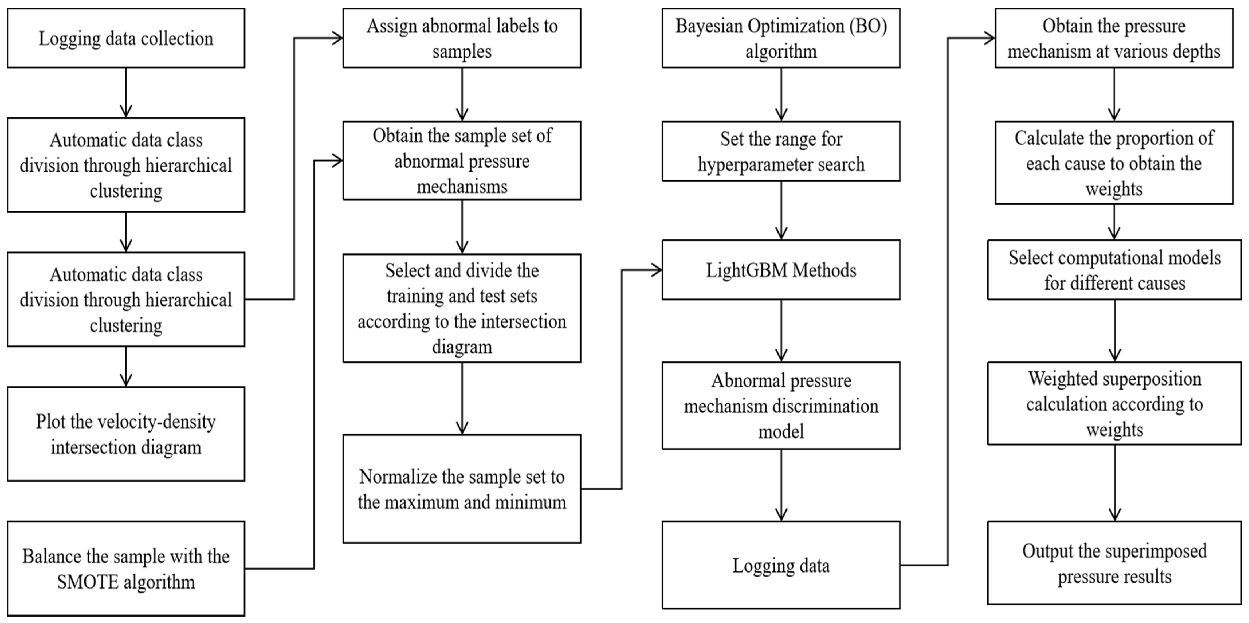
Currently, in the process of identifying the causes of abnormal formation pressure using velocity–density cross-plots, the causes of abnormal pressure mechanisms often require manual analysis and interpretation, which is time-consuming and difficult to quantify accurately. Because of this, the introduction of machine learning can greatly improve efficiency and accuracy. The process of establishing a method for identifying the causes of abnormal formation pressure based on artificial intelligence algorithms is shown in Figure 2.

3.1. Mining Similar Abnormal Pressure Mechanism Samples Based on Cluster Analysis

By collecting well logging data for the entire depth of the target well, the initial focus is on the variation trend of P wave velocity with depth. By analyzing the changes in P wave velocity with depth, the normal compaction section and abnormal high-pressure section of the formation can be identified. This method helps identify specific areas in the formation where abnormal pressure may exist, providing important clues for subsequent analysis.

To further study the mechanisms causing abnormal high pressure, the key geophysical parameters of velocity and density are utilized. By applying clustering algorithms for unsupervised learning, the abnormal high-pressure mechanisms are divided into different groups, as illustrated in Figure 3. The advantage of this method is that it can automatically cluster similar data samples together without prior knowledge of specific categories.

Hierarchical clustering is an unsupervised learning algorithm used to hierarchically divide data samples into different categories, forming a clustering tree structure. This method incrementally merges or splits data to construct different levels of clusters. Hierarchical clustering has two main methods: agglomerative clustering and divisive clustering. Agglomerate clustering starts with each data point and gradually merges the most similar data points into clusters, continuing this process until all data points are merged into one large cluster. This method is suitable for small datasets but may be less efficient for large datasets. Divisive clustering starts with all data points in one large cluster and gradually splits it into smaller clusters, continuing this process until each data point forms its own cluster. This method is suitable for large datasets but may lead to over-segmentation in some cases. Key steps in hierarchical clustering include defining similarity or distance metrics between data points, such as Euclidean distance, Manhattan distance, and correlation coefficients. Starting from each data point, clusters are incrementally merged or split based on similarity or distance, constructing a clustering tree. The clustering tree can be visualized through a dendrogram, helping to understand the clustering structure of the data. Hierarchical clustering helps identify groups of similar samples, aiding in recognizing different mechanisms causing abnormal high pressure. These clusters can reveal the combined effects of geological features, formation properties, and fluid migration in different abnormal high-pressure sections. The results of this method contribute to a more comprehensive understanding of the mechanisms causing abnormal high pressure, providing valuable references for geological exploration and engineering decisions. It is important to note that while hierarchical clustering can help discover groups of similar samples, geological background knowledge and the expertise of geologists are still needed to interpret the model results and validate hypotheses. By considering multiple factors, more accurate inferences on the causes of abnormal high pressure can be made.

3.1.1. Classifying Different Pressure Mechanism Sample Groups Based on Normal Trend Lines

Using the Gardner equation (Gardner et al., 1974), which describes the velocity–density relationship, a normal trend line of the velocity–density cross-plot is established by fitting the velocity–density curve of the normal compaction section. This normal trend line represents the typical relationship between velocity and density under normal compaction conditions. This line is then applied to the velocity–density cross-plot of the abnormal high-pressure section to supplement additional loading curves. By integrating traditional discrimination approaches, data groups are carefully divided to identify characteristics of different abnormal high-pressure causes. In this process, data are categorized into three main types: undercompaction, fluid expansion, and shale diapirism, forming sample data for establishing a model to determine abnormal pressure mechanisms. A machine learning model is then developed to build a determination model of abnormal pressure mechanisms based on well logging parameters. The aim of this model is to use logging parameters like velocity and density as inputs to accurately classify and identify the different mechanisms causing abnormal pressure. By combining the normal trend line with loading curves of the abnormal high-pressure section, the model is provided with sufficient data samples. These samples include typical relationships between velocity and density under normal geological conditions and disturbances to this relationship under abnormal conditions. These data help train the machine learning model to recognize different abnormal pressure mechanisms within the well logging parameter space. The final model will be a powerful tool for interpreting abnormal formation conditions. By inputting well logging data such as clay content, porosity, velocity, and density, the model can automatically analyze and identify different abnormal pressure mechanisms like undercompaction, fluid expansion, and shale diapirism.

3.1.2. Establishing a Cause Mechanism Identification Model Based on BO-LightGBM

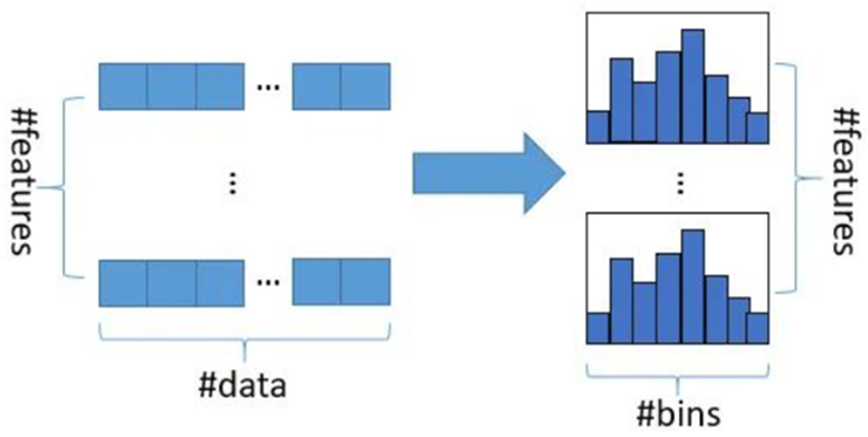
For the given problem of categorizing the causes of abnormal pressure, a decision tree algorithm suitable for treating numerical values as categorical symbols was chosen, combined with gradient boosting and histogram techniques, to construct an efficient and accurate LightGBM model. During model construction, the advantages of decision tree algorithms were fully utilized to map continuous numerical features to categories of abnormal mechanisms. By binning the numerical values, the model can treat these numbers as categorical symbols, better fitting the needs of the problem. LightGBM is an improved version of the gradient boosting tree algorithm that optimizes the algorithm and data structure to enhance training speed and memory efficiency. Below are the principles of the GOSS algorithm: LightGBM adopts the GOSS vertical parallelization training algorithm, which selects a portion of samples with large gradient values for training and samples those with small gradient values to reduce dataset size, maintaining model accuracy while significantly reducing training time and memory consumption. In the histogram optimization algorithm, LightGBM uses the GOH histogram optimization algorithm. Instead of sorting feature values traditionally, it bins feature values into histograms, reducing sorting complexity and increasing training speed, as shown in Figure 4.

(1)

Learning Rate and Early Stopping: LightGBM allows users to set learning rates and early stopping strategies to control the training process, limiting each weak learner’s contribution and avoiding overfitting.

(2)

Feature Parallelization and Histogram Compression: LightGBM employs feature parallelization and histogram compression techniques, enhancing training speed and memory efficiency.

(3)

Leaf-Wise Growth Strategy: LightGBM uses a leaf-wise growth strategy, splitting the leaf with the largest gradient each time, focusing on samples with larger gradients and accelerating learning.

(4)

Depth-Limited Decision Trees: LightGBM uses depth-limited decision trees to reduce memory consumption and model complexity.

(5)

Parallel Learning and Cache Optimization: LightGBM increases training efficiency through parallel learning and cache optimization, updating multiple leaf nodes’ statistics simultaneously and reducing data reads.

Overall, LightGBM significantly improves training speed and memory efficiency through GOSS and GOH algorithms, the leaf-wise growth strategy, feature parallelization, and histogram compression, excelling in handling large-scale datasets and high-dimensional features. However, LightGBM’s parameter combinations are complex and rely on manual experience, with exhaustive optimization taking considerable time. Intelligent optimization algorithms play a crucial role in machine learning by optimizing model parameters, architectures, and hyperparameters, improving performance, reducing training time, and enhancing generalization. These algorithms balance exploitation and exploration, finding the best combinations in complex parameter spaces for better prediction and classification.

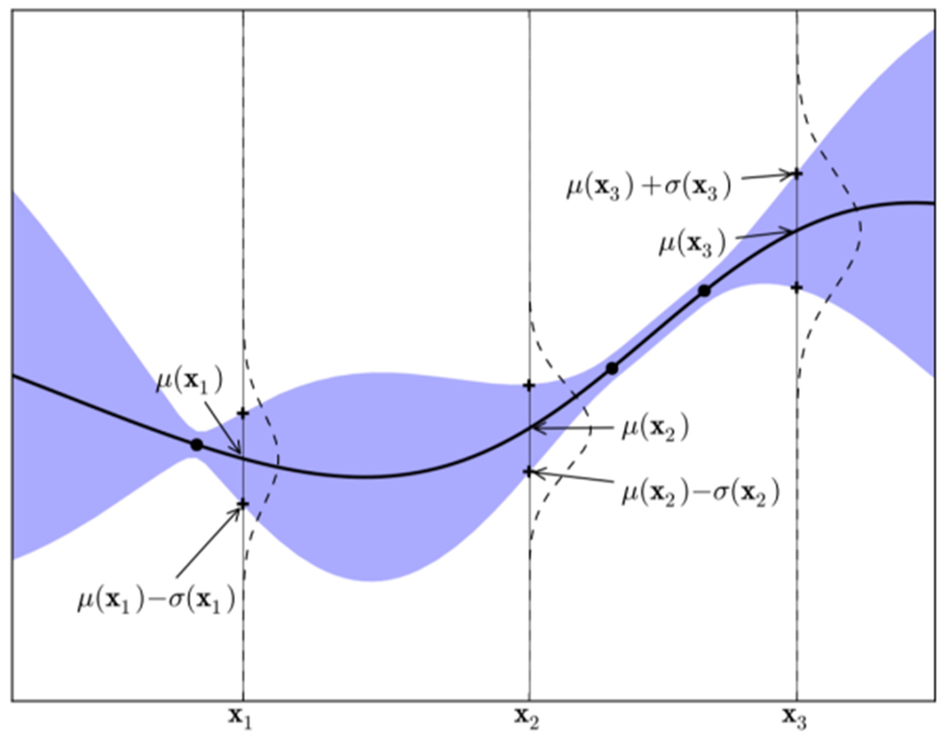
Probability surrogate models and acquisition functions are core components of Bayesian optimization. Among them, surrogate models can be parametric or non-parametric, with Gaussian processes being the most widely used non-parametric model. Acquisition functions map from input, observation, and hyperparameter space to real number space, balancing exploitation and exploration to evaluate the distribution of points. Bayesian optimization using Gaussian processes as surrogates has several advantages. First is flexibility: a Gaussian process is a non-parametric model that does not require a predefined specific functional form. This allows the Gaussian process to adapt to various complex functional relationships, including non-linear, non-convex, and noisy conditions. Because Gaussian processes can fit any continuous function, they offer great flexibility in optimization problems. Second is uncertainty estimation: a Gaussian process can not only predict the expected value of the objective function but also provide an uncertainty estimate of the prediction results. Through a Gaussian process, the posterior probability distribution of each sample point can be obtained, allowing for modeling the confidence in the prediction results. This is very useful for optimization algorithms, as they can explore more samples in areas with high uncertainty to improve global optimization accuracy. Finally, sampling efficiency: a Gaussian process model can select the next sampling point based on confidence, making the sampling process more efficient. By using a Gaussian process model, Bayesian optimization algorithms can choose the most likely locations to achieve the global optimum, not just local optima. This reduces unnecessary sampling and finds better solutions within limited sampling times. The Gaussian distribution and sampling are shown in Figure 5.

A Gaussian process is a collection of random variables, any finite number of which have a joint Gaussian distribution. The function of a Gaussian process is defined as follows:

$$f(x)~GP(m(x),k(x,x’))$$

(1)

where m(x) is the mean function, usually set to 0, and k(x,x’) is the covariance function, with x’ being a random variable. Considering the prior distribution with a mean of p(f | X, β):

$$p(f|X,\beta )=N(0,\sum )$$

(2)

where X is the training set, f is the set of function values of the unknown function, and K is the matrix formed by ∑k(x,x’).

When observation noise ϵ is present, p(ε) = N(0, σ²), where σ² is the variance, the likelihood distribution is given by:

$$p(y|f)=N(f,{\sigma }^{2}I)$$

(3)

where y is the set of observations, and I is the identity matrix.

The marginal likelihood can be obtained as follows:

$$p(y|X,\beta )=N(0,\sum +{\sigma }^{2}I)$$

(4)

Based on the properties of Gaussian processes, we can obtain the posterior distribution:

$$\left[\begin{array}{l}y\\ f_{\ast }\end{array}\right]~N\left\{0,\left[\begin{array}{ll}\sum +{\sigma }^{2}I& K_{\ast }\\ K_{\ast }^T& K_{\ast \ast }\end{array}\right]\right\}$$

(5)

where f_∗ is the prediction value, K_∗ is the covariance matrix between the training inputs and the test inputs, $K_{\ast }^T$ is the transpose of K_∗, and K_∗∗ is the covariance between the test inputs. The predictive distribution is given by:

$$f_{\ast }=K_{\ast }^T{(\sum +{\sigma }^{2}I)}^{-1}y$$

(6)

$$\mathrm{cov}(f_{\ast })=K_{\ast \ast }-K_{\ast }^T{(\sum +{\sigma }^{2}I)}^{-1}{K}_{\ast }$$

(7)

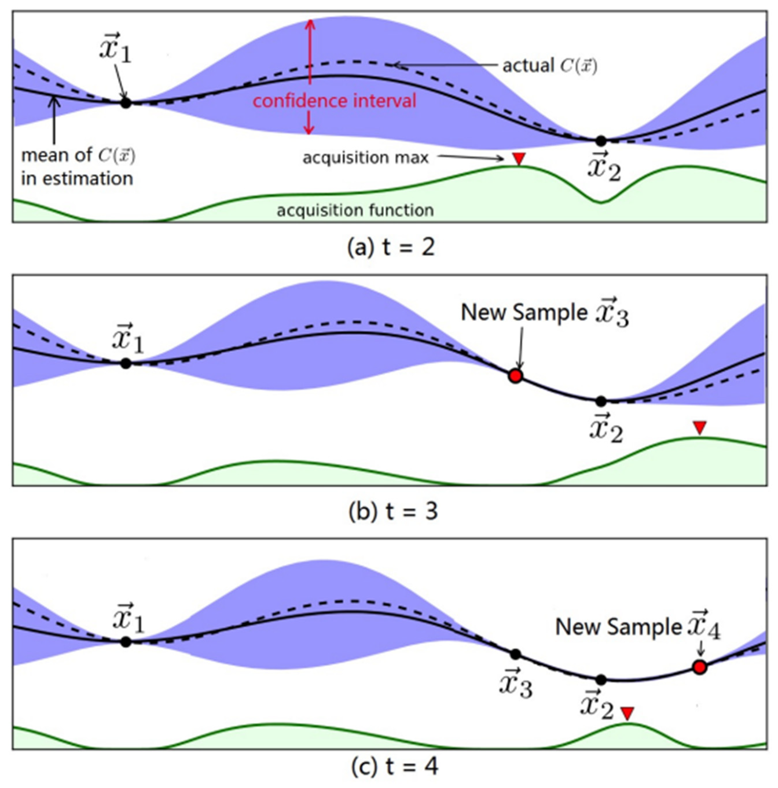
The acquisition function is crucial for determining the next evaluation point. When using an upper confidence bound strategy, the next evaluation point is:

$$x_{t+1}=\arg \max {\mu }_t(x)+\sqrt{{\alpha }_t}{\sigma }_t(x)$$

(8)

where α_t is a constant balancing exploration and exploitation, ${\mu }_t(x)$ is the mean, and ${\sigma }_t(x)$ is the standard deviation.

The search process in Bayesian optimization is illustrated in Figure 6.

3.1.3. Calculating Overlapping Weight Relationships Based on the Identification Results of Abnormal Pressure Mechanisms

The trained model is utilized to identify the abnormal pressure causation categories for each depth data point within a certain section of the Rio del Rey Basin in Cameroon. By inferring through the model, each depth data point can be classified to determine its corresponding abnormal pressure causation category. Following this classification, the data across the entire well section are statistically analyzed to compute the frequency of occurrence of each abnormal pressure causation category within the well section. Through these statistics, the proportions of the three primary abnormal pressure causation categories—undercompaction, fluid expansion, and shale diapirism—within the total well section data can be calculated. This calculation allows us to determine the relative weight of each causation category within the well section, aiding in understanding the overlay mechanism of different causes throughout the well section. These weights provide valuable insights into the impact of multiple causations. For instance, a causation category with a high proportion might dominate the well section, whereas a category with a low proportion might have a minor influence. This analysis assists in deeply understanding the interrelationships and influence levels of different abnormal pressure causations within the well section. Machine learning algorithms have unique advantages in classification applications. They can automatically learn data patterns and rules, enabling intelligent decision making. These algorithms can adapt to different data distributions, handle complex features and non-linear relationships, and thus classify data accurately. For large-scale datasets, machine learning algorithms can efficiently process data. Through iterative optimization and diverse algorithms, they can discover potential patterns and enhance classification performance. Therefore, leveraging machine learning algorithms is crucial in identifying abnormal pressure causation mechanisms. This approach provides automation, accuracy, and adaptability, making it a vital tool for addressing the challenges of quantifying abnormal pressure causation mechanisms.

4. Analysis of Abnormal Formation Pressure Mechanisms

Utilizing well logging data, we extracted and calculated essential parameters, including effective well depth, sonic velocity, density, resistivity, and natural gamma radiation. A detailed analysis of the sonic velocity as a function of depth was conducted to identify the location of the normally compacted section, which is determined to be situated at depths exceeding 1300 m. The corresponding data for this normally compacted section are presented in Figure 7. Subsequently, this dataset was employed to establish the Gardner correction equation, facilitating the derivation of the normal trend line for the velocity–density relationship. This trend line serves as a critical reference point for identifying and analyzing abnormal pressures in the subsequent stages of the study.

Using hierarchical clustering algorithms to cluster data, determining the number of clusters in the clustering algorithm before clustering is a crucial step, which directly affects the quality and application effect of the final clustering results. This paper combines the elbow method and silhouette method to determine the optimal number of clusters. Figure 8 is the elbow method graph, which plots the distortion values corresponding to each number of clusters. The number of clusters is on the X axis, and the distortion values are on the Y axis. By observing the shape of the elbow graph, the elbow point usually refers to the position where the curve changes sharply at an inflection point. The number of clusters corresponding to the elbow point is generally considered to be the optimal number of clusters. According to the elbow method graph, the optimal number of clusters is n = 6. On the basis of the elbow method, clustering results under different numbers of clusters are compared. When n = 6, hierarchical clustering identifies clusters that conform to the pressure recognition mechanism, and the classification effect on the dataset is more obvious. Some clustering results under different numbers of clusters are shown in Figure 9.

To accurately divide the clustering results of different abnormal pressure mechanisms, a normal compaction trend line is drawn using the Gardner correction equation established by the data from the normal compaction section. The Gardner empirical formula is a method that reveals the relationship between formation density and P wave velocity, and there is often a certain error when directly using the Gardner formula to research velocity–density relationships. Therefore, based on the Gardner formula, the Gardner correction equation is obtained by fitting the normal compaction section data from the #A well and #B well in Cameroon. The Gardner correction equation fitted based on the normal compaction section data is shown in Figure 10.

In the Rio Del Rey Basin, by combining the geological data of the target area and the velocity–density cross-plot, it can be seen that various mechanisms such as undercompaction, fluid expansion, and shale diapirism are superimposed and jointly affect the formation of abnormal high pressure. The corrected Gardner curve is used as a loading curve on the velocity–density cross-plot to identify the abnormal pressure mechanism. As shown in Figure 11, Categories 1, 4, and 5 are on the left and right sides below the normal trend line, deviating towards the lower values of velocity and density relative to the normal compaction trend section of this depth range but still distributed around the loading curve or having a similar trend to the loading curve, and their abnormal causes correspond to undercompaction; Category 3 is slightly below the normal trend line, relatively concentrated near the unloading curve of this depth range, and its abnormal cause corresponds to hydrothermal pressure increase; Categories 0 and 2 are above the normal trend line, similar to the opposite process of fluid expansion, with a certain increase in velocity relative to the normal velocity and a slight increase or unchanged density, and their abnormal causes correspond to shale diapirism.

When processing data from the abnormal high-pressure section, logging parameters such as well depth, velocity, shale content, porosity, and density are selected as features to identify pressure mechanisms. These well-divided abnormal pressure sample data are randomly divided into training and testing set samples in a 7:3 ratio, and the sample training set is balanced by the SMOTE algorithm to ensure the robustness and generalization ability of the model. To eliminate the impact of different data dimensions, the maximum-minimum normalization method is used to standardize the dataset, making each indicator have the same scale, thereby effectively improving the training effect.

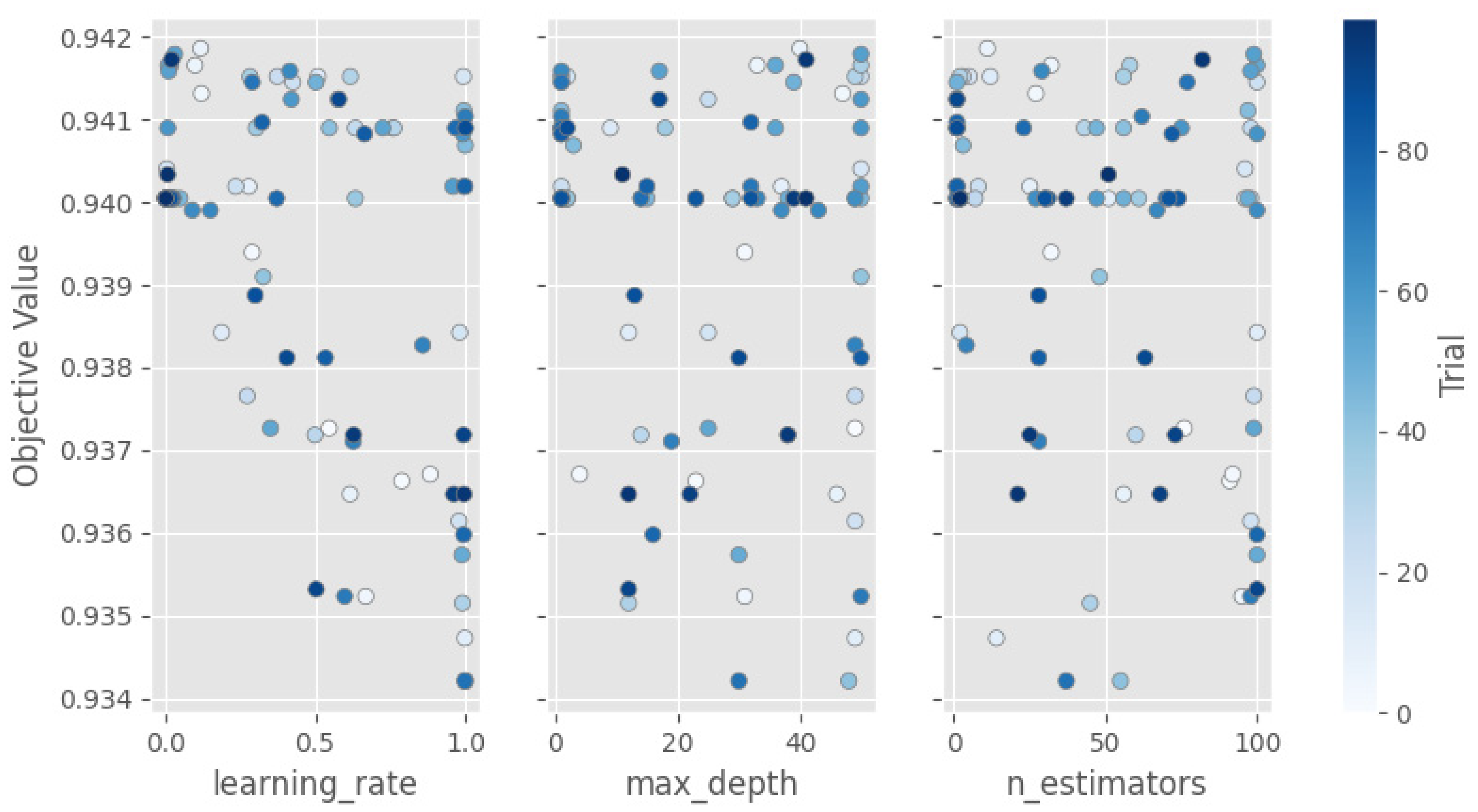
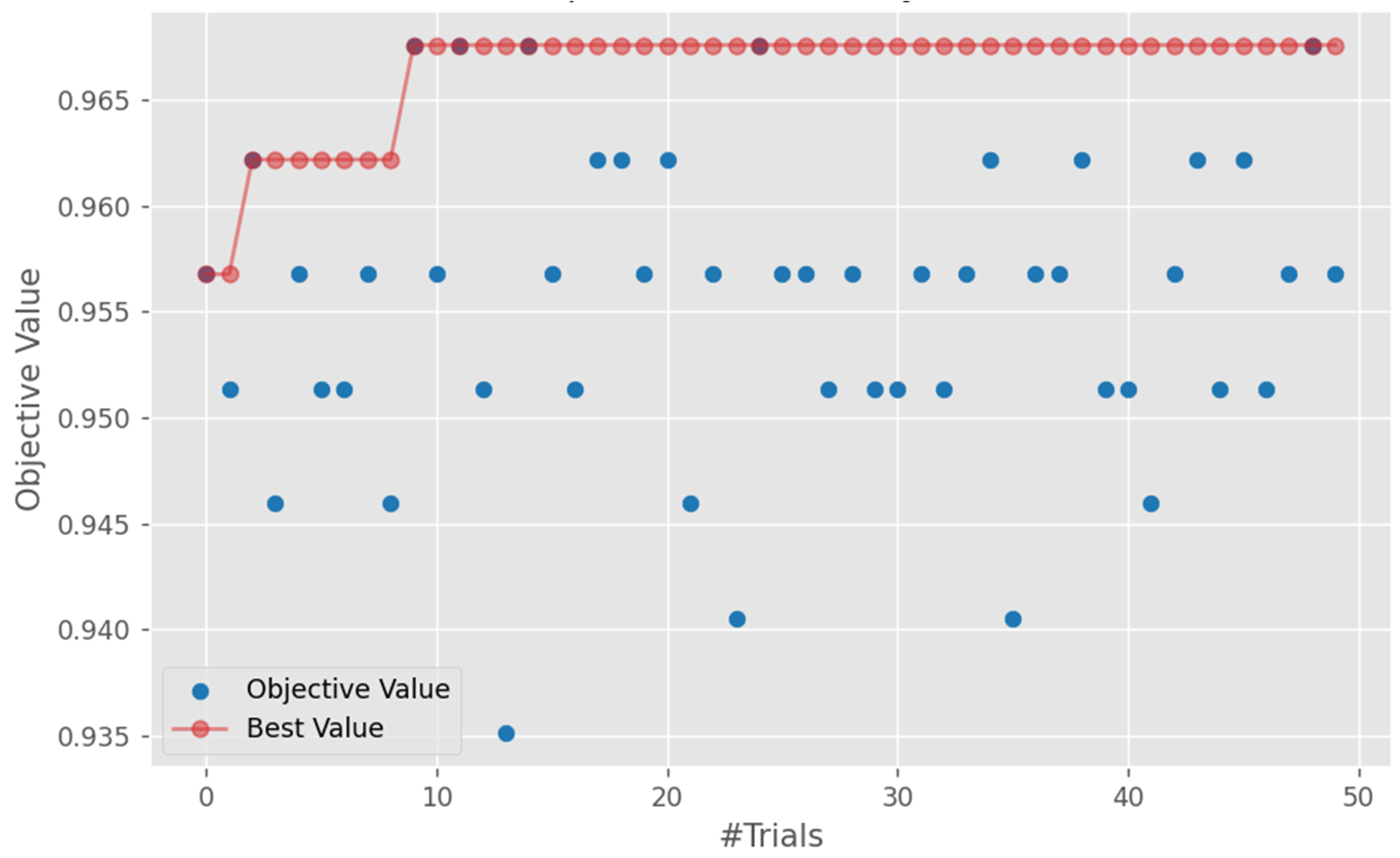
The Bayesian optimization algorithm based on the Gaussian process is introduced to optimize the number of base models, the depth of decision trees, and the learning rate of the LightGBM model. The search ranges for these parameters are [1, 100], [1, 50], and [0, 1], respectively. Through 50 iterations of the Bayesian optimization algorithm, the combination parameters of the LightGBM model with the highest recognition accuracy are finally obtained.

The search and optimization process of the Bayesian optimization algorithm is shown in Figure 12 and Figure 13. Figure 12 is a slice graph of the parameter relationships in the model, representing the progress of different hyperparameters in multiple trials. The horizontal coordinates are the learning rate, tree depth, and tree number, three hyperparameters in the model, and the vertical coordinates are the target function values, representing the model accuracy, with the legend on the right representing the number of iterations; Figure 13 is a historical record graph of model hyperparameter optimization, representing the performance improvement process of the model in multiple iterations. The horizontal coordinate is the number of iterations, and the vertical coordinate is the target function value, representing the model accuracy, with the blue point representing the current iteration accuracy and the red point representing the historical best accuracy.

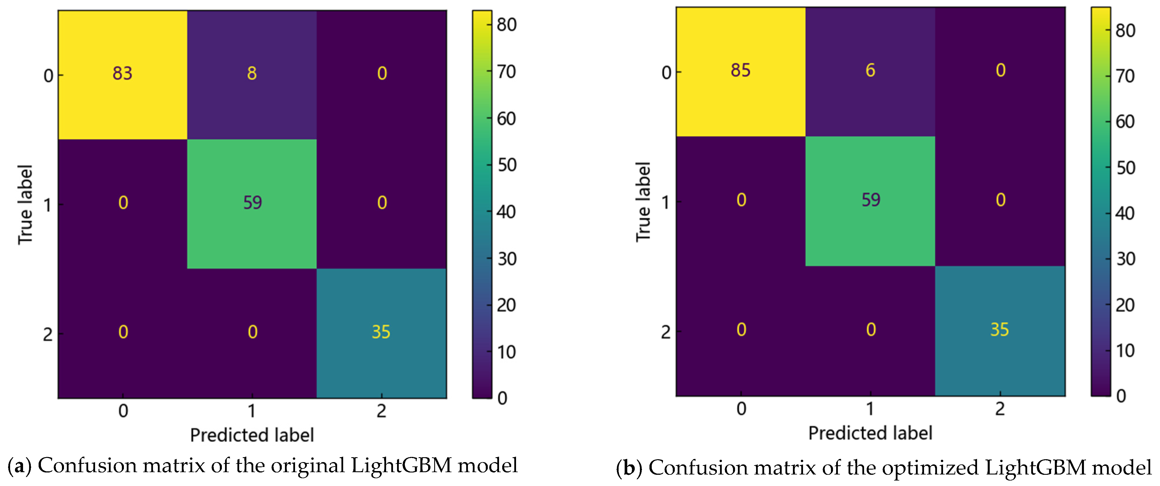
After comparative testing, the original LightGBM model has an accuracy rate of 0.906 on the test set. However, after model optimization using the Bayesian optimization algorithm, the new model achieved a higher accuracy rate on the same test set, reaching 0.942. This means that the new model is more accurate and reliable in identifying the mechanisms of abnormal pressure. Figure 14 is the confusion matrix of the results of the two models in identifying the abnormal pressure mechanism in the test set, used to evaluate the performance of the classification model. The horizontal and vertical axes represent the predicted values and true values of the model, respectively, with 0, 1, and 2 representing the abnormal pressure mechanisms of undercompaction, hydrothermal pressure increase, and shale diapirism, respectively. The color bar on the right explains the range of sample quantities corresponding to the color of each cell in the confusion matrix. It can be found that the optimized model is superior to the original model in the three abnormal pressure mechanisms, indicating that it is feasible to identify the mechanisms of abnormal pressure through machine learning.

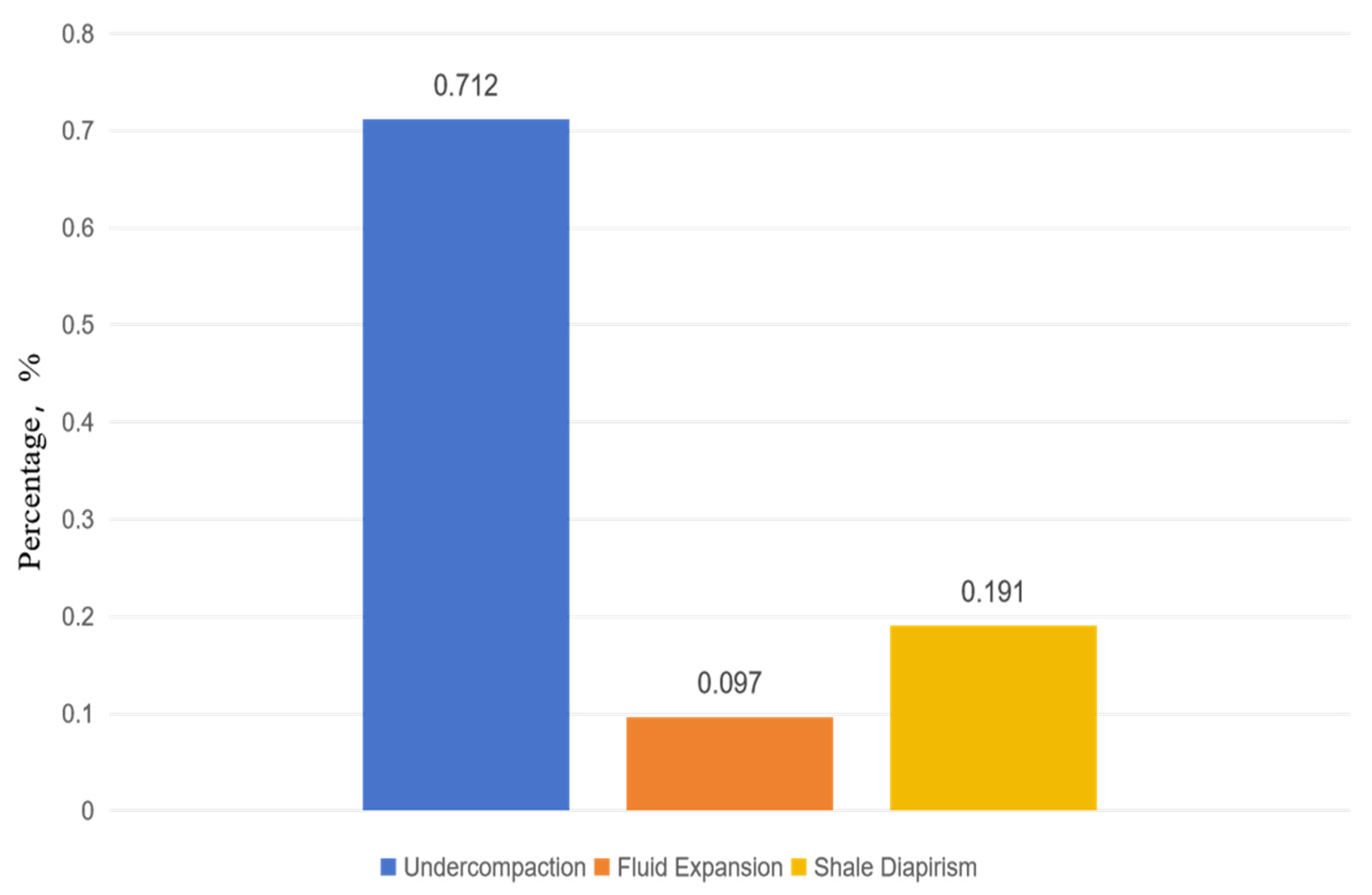
In the Rio Del Rey Basin, various mechanisms such as undercompaction, fluid expansion, and shale diapirism are superimposed and jointly affect the formation of abnormal high pressure. By calculating the weights of the high-pressure mechanism categories at different well depths in the high-pressure layer segments of the #A well, #B well, and BRM1 well in the Rio Del Rey Basin, the relative importance of each mechanism in the formation of abnormal high pressure can be determined. The experimental results show that undercompaction is the dominant mechanism for abnormal high pressure in the Rio Del Rey Basin, accounting for about 70%, while fluid expansion and shale diapirism account for 10% and 20%, respectively. The proportion of each mechanism is shown in Figure 15. This means that in this area, undercompaction is the main factor causing abnormal high pressure, and the tectonic compression caused by shale diapirism and the fluid expansion caused by hydrothermal pressure increase further promote the increase in pore fluid pressure in the strata. This finding is of great significance for a deeper understanding of the geological pressure characteristics and sedimentary action in this area. Through the weight analysis of these mechanisms, the formation process of abnormal high pressure can be more accurately predicted and explained, providing strong support for geological research and engineering applications.

According to the aforementioned method for identifying overpressure mechanisms, the causes of overpressure at different strata of the #A well in the work area have been identified and analyzed using the limited data available, and the calculation results are shown in

Table 1. Calculated weights of overpressure mechanisms for five drilled wells.

Well Number	Stratum	Undercompaction Mechanism Weight	Hydrothermal Pressurization Mechanism Weight	Shale Diapirism Mechanism Weight
#A	S1	79.25%	11.64%	9.12%
	M2	69.52%	2.14%	28.34%
	S2	72.05%	8.7%	19.25%
	M3	79.43%	10.64%	9.93%
	S3	75.92%	8.38%	15.71%
	S4	83.9%	4.57%	11.53%
	M5	70.67%	8.03%	21.3%
	S5	73.81%	10.95%	15.24%

.

5. Conclusions

(1)

In the Rio Del Rey Basin in Cameroon, a meticulous data collection process was conducted on three wells, successfully extracting critical logging parameters such as well depth, acoustic velocity, density, resistivity, and natural gamma. These features are essential for discerning the mechanisms behind abnormal formation pressures and have been rigorously analyzed to ensure their utility in subsequent analytical models.

(2)

A pioneering analytical methodology was developed, combining hierarchical clustering with the powerful predictive capabilities of the LightGBM algorithm. This hybrid approach was further refined through Bayesian optimization, achieving an impressive model accuracy of 0.942. This advancement does not only enhances the accuracy of abnormal formation pressure cause identification but also underscores the potential of integrating sophisticated computational techniques with geophysical analysis.

(3)

The study delved into a quantitative analysis of the abnormal formation pressure causes in the #A, #B, and #C wells, revealing that the undercompaction mechanism predominates, with approximately 70%. Fluid expansion and shale diapirism were allocated 10% and 20%, respectively, offering a granular breakdown of the contributing factors to the overpressure phenomena within the basin.

(4)

The findings underscore the multifaceted nature of overpressure mechanisms in sedimentary basins, advocating for a comprehensive approach to their analysis. The methodology presented is readily adaptable to other geological contexts, suggesting avenues for future research that may include expanded data sets, additional machine learning algorithms, and broader stratigraphic evaluations to consolidate the model’s forecasting robustness.

(5)

The research culminates in a significant contribution to geophysical analysis, particularly in identifying the causes of abnormal formation pressures with higher precision. The synergistic application of hierarchical clustering, machine learning, and Bayesian optimization has been demonstrated as an effective strategy for enhancing the accuracy of geological interpretations, providing valuable insights for hydrocarbon exploration and contributing to the strategic planning of production activities in analogous geological settings.

References

1. Swarbrick, R. Review of pore-pressure prediction challenges in high-temperature areas. Lead. Edge 2012, 31, 1288–1294. [Google Scholar] [CrossRef]
2. Ugwu, G.Z. An overview of pore pressure prediction using seismicallyderived velocities. J. Geol. Min. Res. 2015, 7, 31–40. [Google Scholar]
3. Teige, G.M.G.; Hermanrud, C.; Wensaas, L.; Bolas, H.N. The lack of relationship between overpressure and porosity in North Sea and Haltenbanken shales. Mar. Pet. Geol. 1999, 16, 321–335. [Google Scholar] [CrossRef]
4. Bowers, G.L. Determining an appropriate pore-pressure estimation strategy. In Proceedings of the Offshore Technology Conference, OTC, Houston, TX, USA, 30 April–3 May 2001. [Google Scholar]
5. Zhi, Y.; Honghai, F.; Gang, L.; Yunlong, W. Estimating formation pore pressure in tectonic compression zones. Pet. Sci. Technol. 2012, 30, 766–774. [Google Scholar] [CrossRef]
6. Zhang, F.; Lu, X.; Botterill, S.; Gingras, M.; Zhuo, Q.; Zhong, H. Horizontal tectonic stress as a cause of overpressure in the southern margin of the Junggar Basin, northwest China. J. Pet. Sci. Eng. 2021, 205, 108861. [Google Scholar] [CrossRef]
7. Tao, Z.; Fan, H.; Liu, Y.; Zhou, F.; Chen, Y. Carbonate Formation Pressure Prediction Method Based on Machine Learning. In Proceedings of the ARMA/DGS/SEG International Geomechanics Symposium, ARMA, Al Khobar, Saudi Arabia, 30 October–2 November 2023. [Google Scholar]
8. Guo, S.; Wang, Q.; Li, H. A Review of Pore Pressure Prediction Methods for Deepwater Oil and Gas Exploration. J. Pet. Sci. Eng. 2022, 215, 110559. [Google Scholar]
9. Ai, N.; Chen, Z.; Liu, H. Machine Learning Approaches for Predicting Abnormal Pressure in Complex Geological Environments. Appl. Sci. 2023, 13, 2258. [Google Scholar]
10. Chen, X.; Li, Y.; Wang, J. Predicting Pore Pressure Using Support Vector Machines and Neural Networks in Complex Geological Settings. J. Pet. Explor. Prod. Technol. 2023, 13, 375–388. [Google Scholar]
11. Liu, J.; Zhang, H.; Yang, Y. Deep Learning Techniques for Analyzing Logging Data and Predicting Abnormal Pressure Conditions. J. Nat. Gas Sci. Eng. 2023, 110, 104431. [Google Scholar]
12. Li, H.; Guo, S.; Wang, Q. Hydrocarbon Generation and Its Impact on Formation Pressure in Source Rocks. Pet. Explor. Dev. 2022, 49, 943–955. [Google Scholar]
13. Fan, H.; Zhai, J.; Wang, T. Classifying Abnormal Formation Pressures: Mechanisms and Applications. Pet. Sci. Technol. 2017, 35, 177–186. [Google Scholar]
14. Deng, S.; Fan, H.; Liu, Y.; He, Y.; Zhang, S.; Yang, J.; Fu, L. Two innovative pore pressure calculation methods for shallow deep-water formations. J. Appl. Geophys. 2017, 146, 208–213. [Google Scholar] [CrossRef]
15. Pop, J.; Laastad, H.; Eriksen, K.O.; O’Keefe, M.; Follini, J.M.; Dahle, T. Operational Aspects of Formation Pressure Measurements While Drilling. In Proceedings of the SPE/IADC Drilling Conference and Exhibition, Amsterdam, The Netherlands, 23–25 February 2005. [Google Scholar]
16. Deng, S.; Fan, H.; Zhou, Y.; Zhang, M.; Liu, J.; Niu, J. Pore Pressure Calculation Method for Deepwater Shallow Layers with Log Data. In Proceedings of the Offshore Technology Conference, Houston, TX, USA, 4–7 May 2015. [Google Scholar]
17. Yin, Q.; Yang, J.; Tyagi, M.; Zhou, X.; Hou, X.; Wang, N.; Cao, B. Machine learning for deepwater drilling: Gas-kick-alarm Classification using pilot-scale rig data with combined surface-riser-downhole monitoring. SPE J. 2021, 26, 1773–1799. [Google Scholar] [CrossRef]
18. Meister, M.; Lee, J.; Krueger, V.; Georgi, D.; Chemali, R. Formation pressure testing during drilling: Challenges and benefits. In Proceedings of the SPE Annual Technical Conference and Exhibition, Denver, CO, USA, 5–8 October 2003. [Google Scholar]
19. Yang, J.; Fu, C.; Liu, S.; Zhang, W.; Xie, R.; Wu, Y. Key technological innovation and practice of well construction in ultra-deepwater shallow formations. Acta Pet. Sin. 2022, 43, 1500–1508. [Google Scholar]
20. Meister, M.; Buysch, A.; Pragt, J.; Lee, C.; Lee, J. Lessons Learned from Formation Pressure Measurements While Drilling. In Proceedings of the SPWLA Annual Logging Symposium, Noordwijk, The Netherlands, 6–9 June 2004. [Google Scholar]
21. Yang, J.; Wu, S.; Tong, G.; Wang, H.; Guo, Y.; Zhang, W.; Zhao, S.; Song, Y.; Yin, Q.; Xu, F. Acoustic prediction and risk evaluation of shallow gas in deep-water areas. J. Ocean Univ. China 2022, 21, 1147–1153. [Google Scholar] [CrossRef]
22. Yin, Q.; Yang, J.; Borujeni, A.T.; Shi, S.; Sun, T.; Yang, Y.; Zhao, X. Intelligent Early Kick Detection in Ultra-Deepwater High-Temperature High-Pressure (HPHT) Wells Based on Big Data Technology. In Proceedings of the 29th International Ocean and Polar Engineering Conference, Honolulu, HI, USA, 16–21 June 2019. [Google Scholar]
23. Ma, T.; Chen, P.; Han, X. Simulation and interpretation of the pressure response for formation testing while drilling. J. Nat. Gas Sci. Eng. 2015, 23, 259–271. [Google Scholar] [CrossRef]
24. Hu, Z.; Yang, J.; Li, W.; Li, S.; Feng, P.; Xin, Y. Research and development of compressible foam for pressure management in casing annulus of deepwater wells. J. Pet. Sci. Eng. 2018, 166, 546–560. [Google Scholar] [CrossRef]
25. Abimbola, M.; Khan, F.; Khakzad, N.; Butt, S. Safety and risk analysis of managed pressure drilling operation using Bayesian network. Saf. Sci. 2015, 76, 133–144. [Google Scholar] [CrossRef]
26. Yin, Q.; Yang, J.; Tyagi, M.; Zhou, X.; Wang, N.; Tong, G.; Xie, R.; Liu, H.; Cao, B. Downhole quantitative evaluation of gas kick during deepwater drilling with deep learning using pilot-scale rig data. J. Pet. Sci. Eng. 2022, 208, 109136. [Google Scholar] [CrossRef]
27. Zhang, Y.; Liu, S.; Zhang, F. Identification of overpressure mechanisms in sedimentary basins. J. Nat. Gas Sci. Eng. 2016, 36, 1184–1196. [Google Scholar]
28. Zhang, Y.; Liu, S.; Zhang, F. Mechanisms and Implications of Undercompaction in Sedimentary Basins. J. Nat. Gas Sci. Eng. 2021, 92, 103899. [Google Scholar]
Figure 1. Velocity–density cross-plot variations over well depth.
Applsci 14 10149 g001
Figure 2. Application of clustering algorithms.
Applsci 14 10149 g002
Figure 3. Application of clustering algorithm.
Applsci 14 10149 g003
Figure 4. Histogram optimization in LightGBM.
Applsci 14 10149 g004
Figure 5. Gaussian distribution and sampling.
Applsci 14 10149 g005
Figure 6. Bayesian optimization search process.
Applsci 14 10149 g006
Figure 7. Normal compaction section logging data.
Applsci 14 10149 g007
Figure 8. Elbow method for determining cluster number.
Applsci 14 10149 g008
Figure 9. Clustering results with different numbers of clusters.
Applsci 14 10149 g009
Figure 10. Gardner correction equation.
Applsci 14 10149 g010
Figure 11. Velocity–density cross-plot with trend line.
Applsci 14 10149 g011
Figure 12. Results of all hyperparameter trials with number of tests.
Applsci 14 10149 g012
Figure 13. Process of LightGBM model accuracy improvement.
Applsci 14 10149 g013
Figure 14. Confusion matrices of LightGBM models.
Applsci 14 10149 g014
Figure 15. Weight of multiple causative mechanisms.
Applsci 14 10149 g015