Abstract
Across the globe, landslides cause significant loss of life, injuries, and widespread damage to homes and infrastructure. Therefore, assessing and analyzing landslide hazards is crucial to human, environmental, cultural, economic, and social sustainability. This study utilizes ArcGIS 10.8 and Python 3.9 to create landslide databases for Niigata Prefecture (NIG), Iwate and Miyagi Prefectures (IWT-MYG), and Hokkaido (HKD), drawing on data obtained from the National Research Institute for Earth Science and Disaster Resilience, Japan. A distinguishing feature of this study is the application of a Convolutional Neural Network (CNN), which significantly outperforms traditional machine learning models in image-based pattern recognition by extracting contextual information from surrounding areas, a distinct advantage in image and pattern recognition tasks. Unlike conventional methods that often require manual feature selection and engineering, CNNs automate feature extraction, enabling a more nuanced understanding of complex patterns. By experimenting with CNN input window sizes ranging from 3 × 3 to 27 × 27 pixels and employing diverse sampling techniques, we demonstrate that larger windows enhance the model’s predictive accuracy by capturing a wider range of environmental interactions critical for effective landslide modeling. CNN models with 19 × 19 pixel windows typically yield the best overall performance, with CNN-19 achieving an AUC of 0.950, 0.982 and 0.969 for NIG, HKD, and IWT-MYG, respectively. Furthermore, we improve prediction reliability using oversampling and a random window-moving method. For instance, in the NIG region, the AUC of the oversampling CNN-19 is 0.983, while the downsampling AUC is 0.950). These techniques, less commonly applied in traditional machine learning approaches to landslide detection, help address the issue of data imbalance often seen in landslide datasets, where instances of landslides are far outnumbered by non-landslide occurrences. While challenges remain in enhancing the model’s generalization, this research makes significant progress in developing more robust and adaptable tools for landslide prediction, which are vital for ensuring environmental and societal resilience.
1. Introduction
Landslides are natural phenomena characterized by the downward movement of soil or rock on slopes, influenced by various internal factors such as topography, lithology, and geological structure, as well as external factors like river erosion, groundwater activity, rainwater absorption, earthquakes, and human activities such as artificial slope cutting. These events can cause significant damage, impacting industrial and agricultural production and leading to casualties and destruction of property. The complexity of landslide triggers, which include a combination of natural and human-induced factors, necessitates extensive data collection and sophisticated analysis tools. Reflecting on the development of landslide research, traditional methods of analysis often fall short due to the vast data requirements, complex data structures, and the ambiguity in information sources [1]. Geographic Information Systems (GIS) have become essential for overcoming these challenges, enhancing the reliability and clarity of landslide risk assessments. GIS offer robust capabilities for managing, analyzing, and presenting spatial and attribute data, making them invaluable in landslide hazard assessment, susceptibility mapping, and ensuring the resilience of environmental and human cultural, economic, and social systems.
Currently, researchers worldwide are dedicated to employing diverse methodologies for the assessment and analysis of landslide hazards [2]. For example, Kadavi, Lee, and Lee compared logistic regression and decision tree models for similar landslide mapping in Gangwon-do, South Korea, advancing methods for landslide risk prediction [3]. Their study highlights the efficacy of computational models in geological hazard assessment. Lee and colleagues used a support vector machine (SVM) for detailed landslide susceptibility mapping in Gangwon Province, Korea, enhancing risk management strategies [4]. Their study exemplifies the effective use of SVM in tackling complex geological challenges. To enhance model training, Sameen and colleagues developed a systematic strategy for subdividing samples to improve landslide susceptibility models [5]. Meanwhile, Adnan and his team focused on improving spatial agreement in machine learning-based landslide susceptibility mapping to achieve more precise predictions [6]. Both of these studies offer innovative refinements to data handling and modeling techniques for more accurate landslide risk assessments. Wei and colleagues introduced a feature enhancement framework for more accurate landslide detection, focusing on improving model performance through feature refinement [7]. In 2022, they also explored combining spatial response features with machine learning for more reliable landslide susceptibility mapping [8]. He and associates developed a unified network that integrates superimposed landslide factors and pixel spatial neighborhood data to enhance precision in landslide susceptibility assessments. Together, these studies advance the use of sophisticated analytical techniques for better predicting and understanding landslide risks [9]. Jiang and Jiang demonstrated the effectiveness of convolutional neural networks (CNNs) in accurately identifying and assessing landslides, highlighting their superior performance over traditional methods [10,11]. Hussain evaluated various models for landslide susceptibility mapping, underscoring the strengths and weaknesses of CNNs and traditional techniques [12]. Ghorbanzadeh and his team further confirmed the superior ability of CNNs to detect landslides and capture complex data patterns, emphasizing the promise of deep learning in improving landslide detection and monitoring [13]. Liu and his team demonstrated that CNNs provide superior predictive accuracy in landslide susceptibility mapping compared to traditional machine learning methods [14].
Building on a foundation of diverse methodologies in landslide hazard assessment, our research innovates by applying convolutional neural networks (CNNs) with variable input window sizes and tailored sampling methods across different regions. This approach departs from the traditional use of static models and universal techniques seen in previous studies, enhancing both the accuracy and applicability of the models by adapting them to regional characteristics. Compared to traditional machine learning approaches, CNNs offer significant advantages by facilitating focused learning and analysis of specific features within targeted areas as well as their surrounding contexts. This capability is invaluable in landslide risk assessment, where causative factors of landslides are often complex and influenced by both local and adjacent regional conditions. By leveraging CNNs, our models can more effectively capture these multifaceted influences, thereby providing a more nuanced and accurate evaluation of landslide risks. Integrating geological data, remote sensing, GIS, and advanced computational models, this research demonstrates how CNNs outperform traditional methods in detection and prediction accuracy, making substantial contributions to landslide risk assessment and management.
In this study, we present a novel approach to assessing landslide risk by creating a comprehensive database for three distinct regions in Japan: Niigata Prefecture (NIG), Iwate and Miyagi Prefectures (IWT-MYG), and Hokkaido (HKD). Departing from traditional methodologies, our strategy incorporates a convolutional neural network (CNN) that utilizes various input window sizes. This method divides the entire study area into smaller image segments, enhancing the analysis of spatial features and increasing the model’s sensitivity to subtle landscape details. To address the common challenge of data imbalance in landslide prediction, we implement two distinct sampling strategies: downsampling, which reduces the prevalence of non-landslide data, and oversampling, using a random window-moving method to ensure a balanced representation of both landslide and non-landslide scenarios. This innovative combination of techniques markedly improves the model’s adaptability across different terrains and mitigates some of the primary obstacles in landslide detection. Our preliminary results indicate that larger window sizes boost the model’s predictive capabilities. CNN models employing 19 × 19 pixel windows typically yield the best overall performance. The incorporation of the random window-moving method has also been proven to enhance the accuracy of our landslide predictions. Moving forward, we plan to delve deeper into the implications of these findings, with the goal of developing more robust and adaptable tools for landslide risk assessment.
2. Study Area and Data
2.1. Study Area
The primary objective of this study is to utilize Convolutional Neural Networks (CNN) to assess the risk of landslide disasters in Japan. Three regions were selected based on specific criteria: Niigata Prefecture (NIG area), Iwate and Miyagi Prefectures (IWT-MYG area), and Hokkaido (HKD area). These areas, illustrated in Figure 1, were chosen due to their historical susceptibility to landslides, availability of comprehensive data sets, and geographic diversity, which includes varied topographical and climatic conditions. Additionally, these regions have experienced significant earthquakes in the past, accompanied by numerous earthquake-induced landslides, making them pertinent study areas for future research on earthquake-triggered landslides. This selection is intended to ensure that the findings are robust and applicable across different landscapes, thus enhancing the study’s relevance and applicability to landslide risk assessment.

Figure 1.
Study areas and distributions of historical landslides: (A) NIG study area, (B) IWT-MYG study area, and (C) HKD study area .
2.1.1. Niigata Prefecture (NIG Area)
The first study area, shown in Figure 1A, is Tokamachi, Kawaguchi, Horinouchi, Ojiya, Yamakoshi, and Nagaoka in Niigata Prefecture, located in central Japan. The latitude and longitude ranges are 138° 40.019′ E to 138° 58.08′ E and 37° 0.6048′ N to 37° 35.2644′ N, respectively. The total area of the region is 1795.36 . The elevation range of the study area is from 14 to 1021.5 m, while the slope range is from 0 to 78.01 degrees.
2.1.2. Iwate Prefecture, Miyagi Prefecture (IWT-MYG Area)
The second study area, shown in Figure 1B, is Ichinoseki, Oshu, and the surrounding area of Iwate Prefecture, and Kurihara and the surrounding area of Miyagi Prefecture, located in northeastern Japan. The latitude and longitude ranges are 140° 40.019′ E to 141° 15.888′ E and 38° 41.1228′ N to 39° 10.869′ N, respectively. The total area is 2447.05 km2. The elevation range of the study area is from 10 to 1627.1 m, while the slope range is from 0 to 71.32 degrees. In the following, “IWT-MYG” is abbreviated as “IWT”.
2.1.3. Hokkaido (HKD Area)
The third study area, shown in Figure 1C, is Mukawa, Abira, and Atsuma in Hokkaido, in the northern part of Japan, with the longitude and latitude ranges of 41° 44′ 11.6″ E to 142° 20′ 2.4″ E and 42° 31′ 42.6″ N to 42° 59′ 13.7″ N, respectively. The total area is 1353 km2. The study area’s elevation ranges from 0 to 1016 m, while the slope ranges from 0 to 76.05 degrees.
2.2. Historical Landslide Records (HLS)
The landslide data utilized in this research were sourced from the National Research Institute for Earth Science and Disaster Resilience, Japan. The landslide topographic distribution map [15] was created through the three-dimensional interpretation of 1:40,000 monochrome aerial photographs captured in the 1970s. This map delineates cliffs and mobile objects, showcasing their spatial distribution on a 1:50,000 topographic map. Through this landslide topographic distribution map, we gain insights into the historical locations, magnitudes, and alterations of landslides. Refer to Figure 1 for visualization.
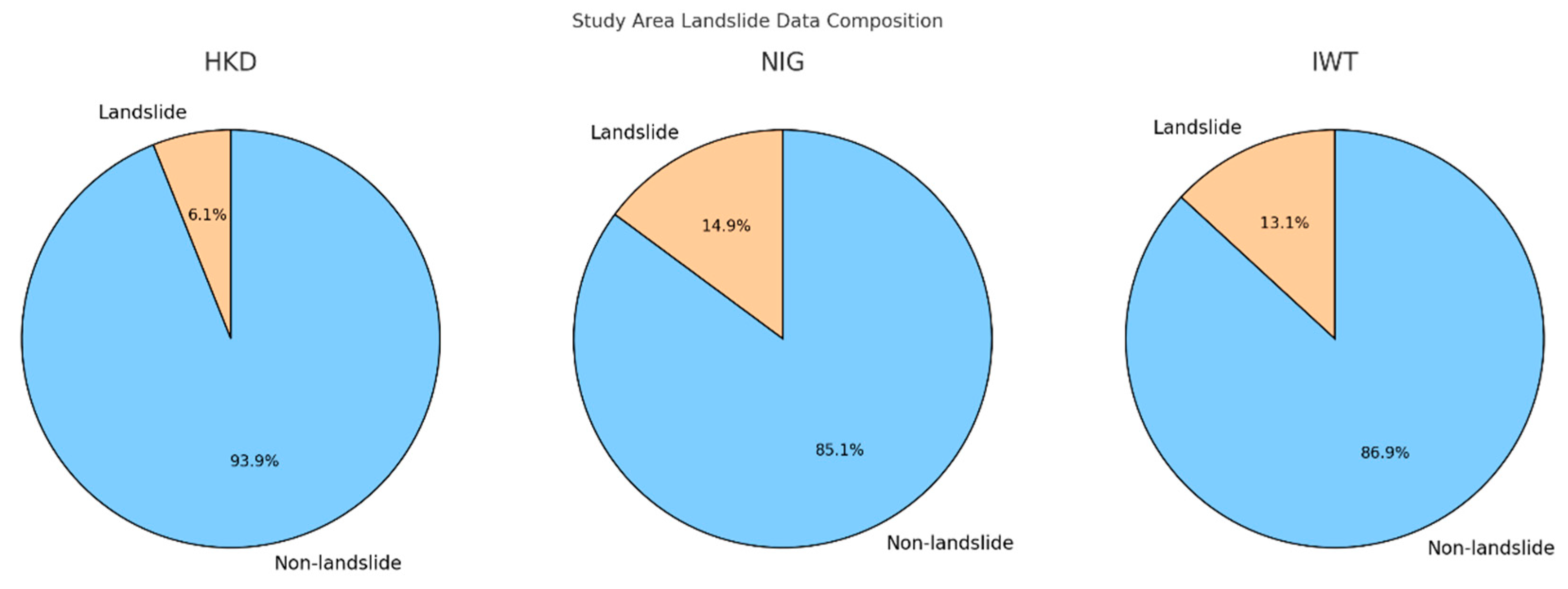
The HKD area has approximately 1.51 million pixels identified as landslide zones out of about 25.02 million total pixels. The NIG area shows around 1.85 million landslide pixels against roughly 12.47 million total pixels. Lastly, the IWT area records the highest with about 3.48 million landslide pixels from a total of nearly 26.50 million pixels. The proportion of landslide and non-landslide pixels is shown in Figure 2.

Figure 2.
Distribution of landslide and non-landslide data.
2.3. Data-Use
Landslides can arise from a multitude of factors, each interconnected with the other in complex ways. Through the examination of landslide causation, certain factors have emerged as particularly relevant for research purposes. These factors can be categorized as follows:
- (1)
- Internal Factors: (a) Topography, (b) Lithology, (c) Geological structure
- (2)
- External Factors: (a) Induced Causes: Earthquakes and precipitation, (b) Human Causes, among
Precipitation’s role in landslide occurrence has been extensively studied worldwide over many years, and this study similarly acknowledges its significance as a key influencing factor. Due to the absence of specific occurrence times for historical landslide data in the study area, the assessment of past landslides initially utilized the average annual precipitation over the past 30 years as a reference.
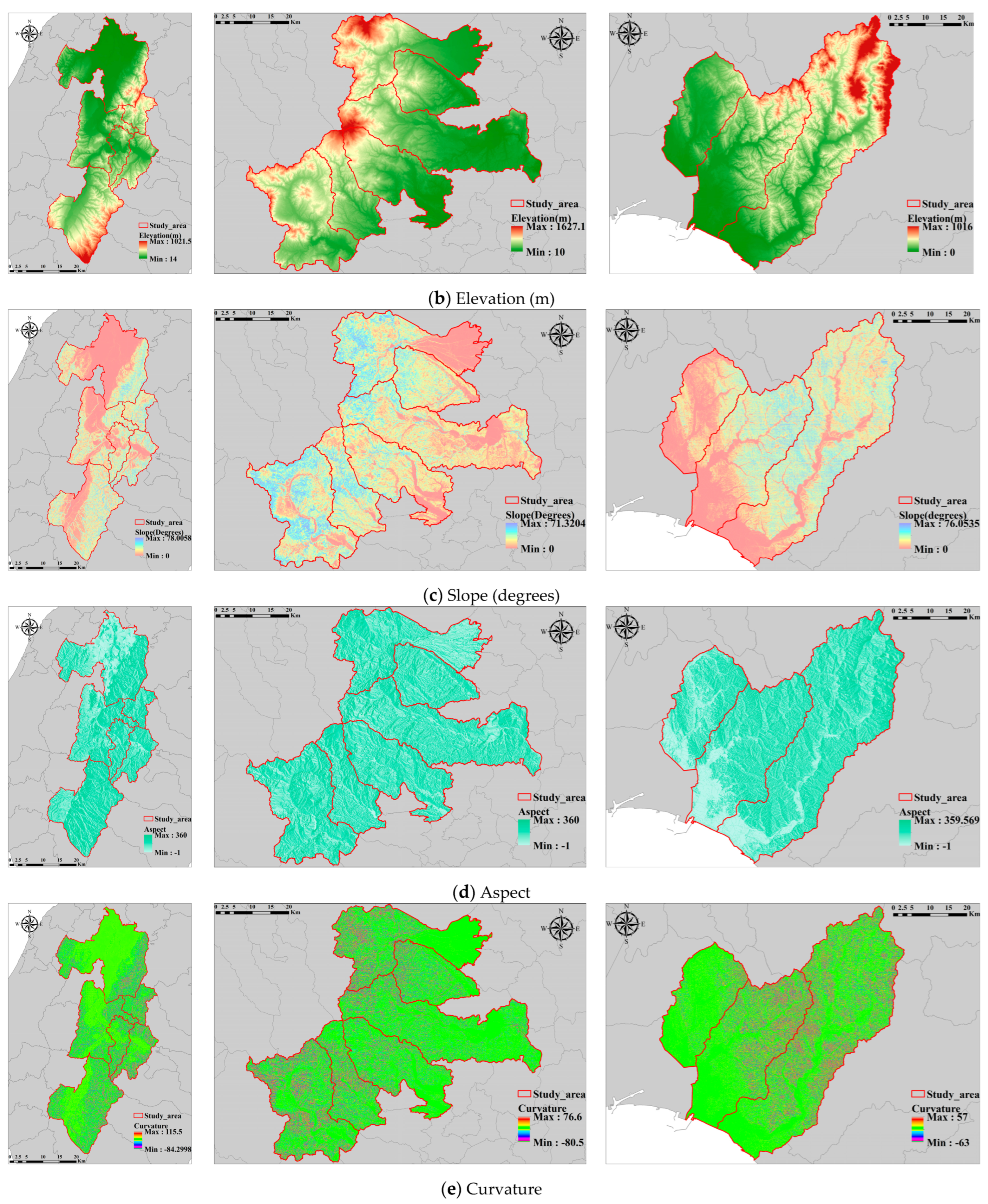
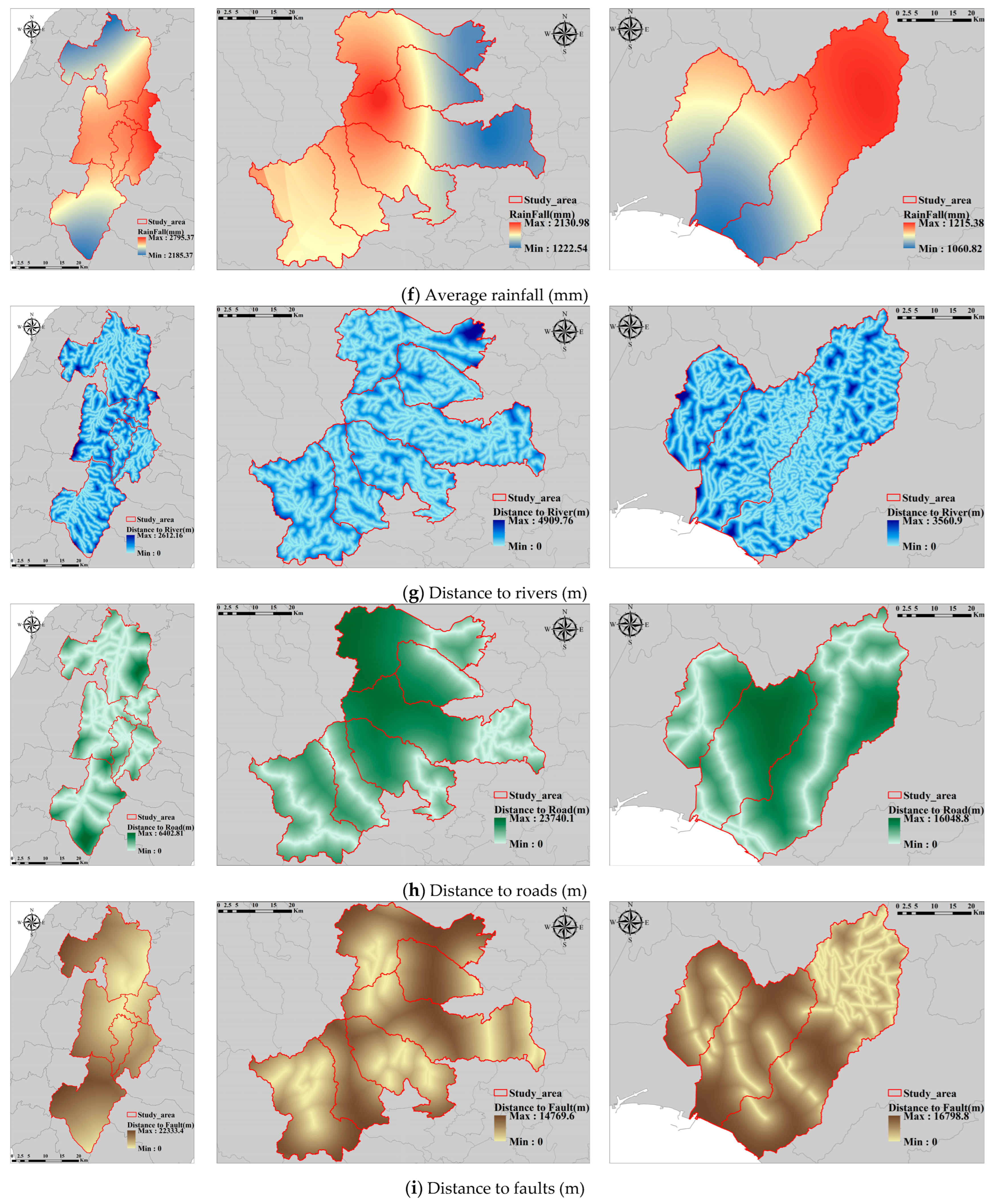
Considering insights from prior research and a diverse range of data sources, this study identifies 14 factors associated with historical landslides: elevation, slope, aspect, curvature, lithology [16], soil type [17], land use [18], precipitation [19,20], distance from rivers [21], faults [22], roads [18], vegetation [23], catchment area [24], and openness [25]. These factors are depicted in Figure 3, Figure A1, Figure A2 and Figure A3 (Appendix A). Table 1 illustrates the range of the dataset. Furthermore, the Digital Elevation Model (DEM) used in this study has a resolution of 10 m, and all landslide records and associated feature resolutions prepared are consistent with the resolution of the DEM.

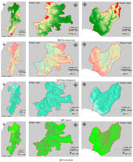
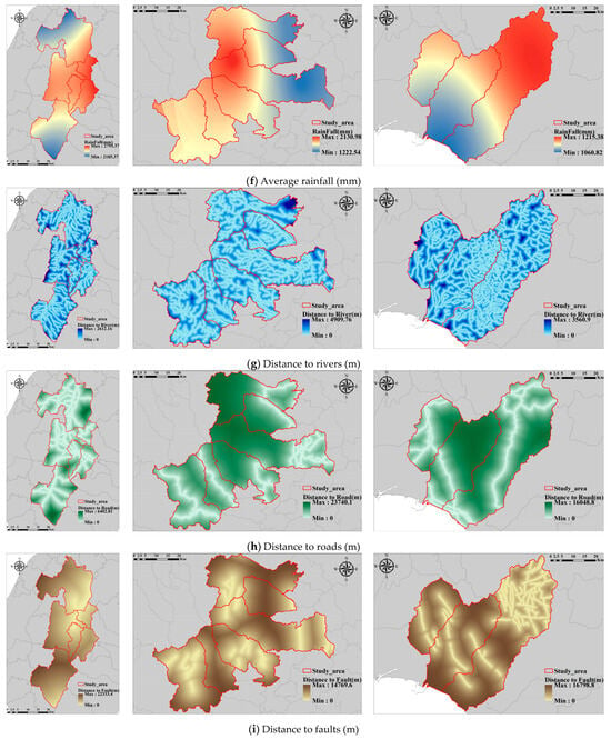
Figure 3.
Maps of landslide features.

Table 1.
Features and data range in the study area.
3. Method
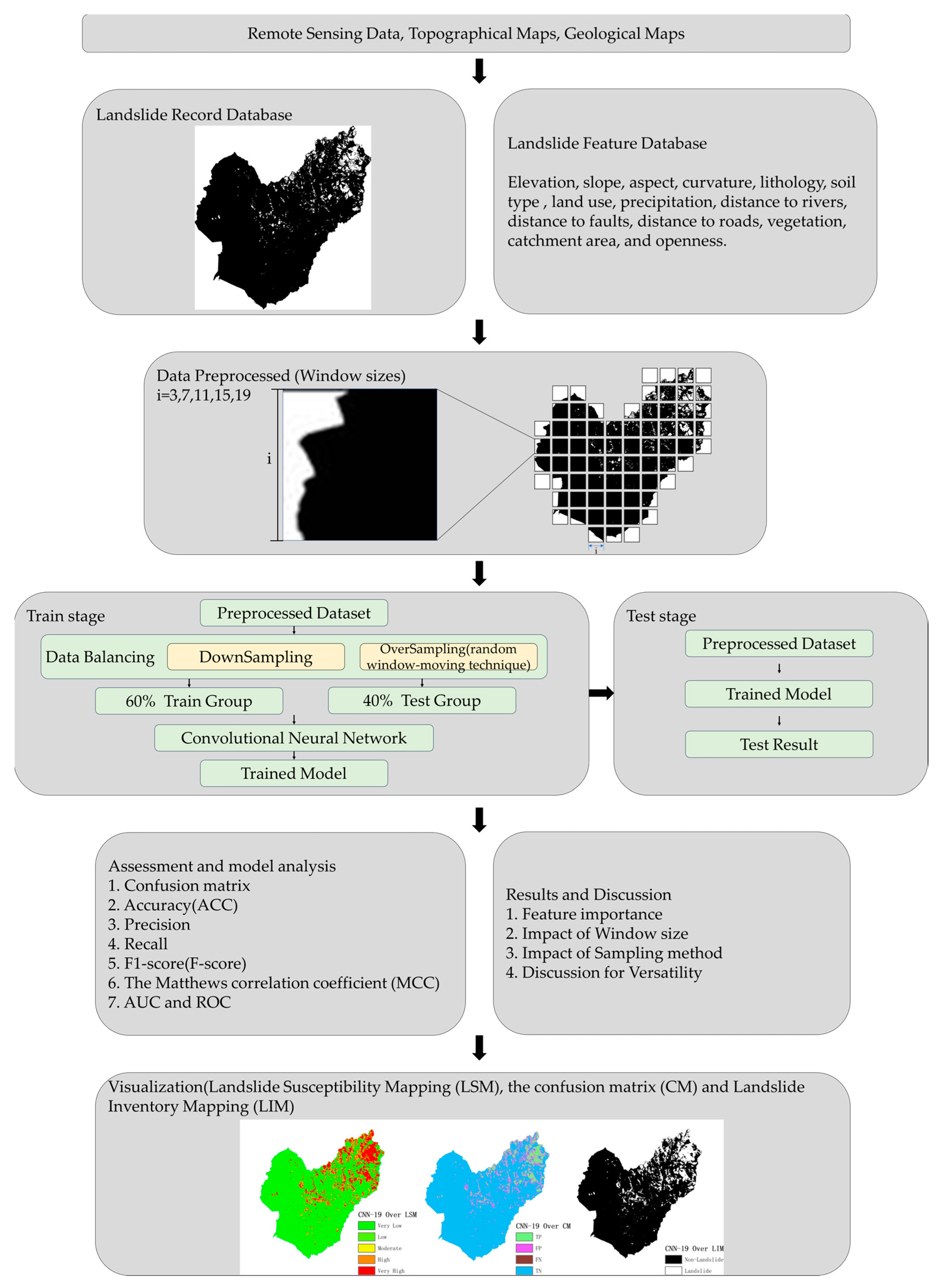
The study process, outlined in Figure 4, is divided into four main stages. First, the database is established by integrating and standardizing all feature data using ArcGIS. In the second stage, the data undergoes preprocessing, where the established Landslide Record Database and Landslide Feature Database are segmented according to predefined window sizes. Third, data balancing is applied, a trained model is developed, and its performance is assessed. In the final stage, the preprocessed data is fed back into the trained model for testing and prediction.
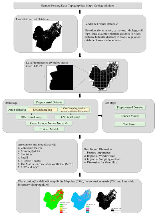
Figure 4.
Flowchart of this study.
3.1. Convolutional Neural Network
The Convolutional Neural Network (CNN) is a type of artificial neural network known for its ability to effectively extract feature representations from images. This capability allows CNNs to recognize visual patterns in images without the need for complex, human-designed rules [26].
The structure of a CNN can be broken down into three main layers: the convolutional layer, the pooling layer, and the fully connected layer. In the convolutional layer, filters are applied to the input image to detect various features. Given a picture size of 500 × 500 and passing through 50 filter convolution layers, the resulting dimension would be 500 × 500 × 50. To manage this large amount of data, the output is downscaled in the pooling layer, effectively reducing the dimensionality while preserving important features. The fully connected layer is responsible for classification, where the features extracted from the previous layers are used to classify objects. The key operations performed in any CNN can be succinctly described by the following equation [27]:
where is the output feature data from the previous layer of the th layer, and indicate the weights of the layers, respectively, that convolve by the linear convolution, and denotes the non-linearity function outside the convolutional layer. These steps are often followed by a pooling operation which is represented by in Equation (1) [27].
In this study, we split the dataset into 60% for training and 40% for testing (train-Prop = 0.6). The model is trained using the Adam optimizer with an initial learning rate of 0.001. The architecture starts with several convolutional layers, beginning with a 512-channel 1 × 1 filter layer with ‘valid’ padding and ReLU activation, followed by a 0.25 Dropout and a 2 × 2 Max Pooling layer to reduce dimensionality and enhance spatial in-variance. Additional convolutional layers include 256, 128, 64, and 32 channel 1 × 1 filters, each followed by a 0.25 Dropout to mitigate overfitting. The network concludes with a Flatten layer, a 256-node Dense layer with ReLU activation, another 0.25 Dropout, and a final 2-node Dense layer with soft max activation suitable for binary classification tasks.
3.2. CNN Window Sizes
In this research, multiple input window sizes were employed for landslide detection, including 3 × 3 pixels, 7 × 7 pixels, 11 × 11 pixels, 15 × 15 pixels, 19 × 19 pixels, 23 × 23 pixels, and 27 × 27 pixels determined through cross-validation. The utilization of various input window sizes was necessitated by the intricate nature of the shapes and sizes of features within the study areas. Notably, the presence of both large and small landslides, often exhibiting diverse shapes, posed a challenge for detection [13]. Some landslides appeared elongated and potentially thin, resembling unsealed roads rather than typical landslide formations. Moreover, the study area exhibited varying aspects, slopes, and flow directions, with individual landslides comprising different aspects. Furthermore, most landslides displayed a blend of topographic features, further complicating their recognition [13]. To address these complexities, various input window sizes were employed, following a similar approach used for detecting complex-shaped objects in urban areas [27]. For clarity, the notation “CNN-i” will be adopted to represent different window sizes: 3 × 3 pixels, 7 × 7 pixels, 11 × 11 pixels, 15 × 15 pixels, 19 × 19 pixels, 23 × 23 pixels, and 27 × 27 pixels, corresponding to CNN-3, CNN-7, CNN-11, CNN-15, CNN-19, CNN-23, and CNN-27, respectively.
Additionally, the DEM data used in this study had a resolution of 10 m × 10 m, where one pixel could cover up to 270 m × 270 m. When employing DEM data with different resolutions, such as 30 m × 30 m, one pixel can cover up to 810 m × 810 m. Therefore, when using different DEM datasets, it is essential to appropriately scale the window sizes to ensure that the spatial representation remains consistent and effective for detecting landslides across various resolutions. This scaling is vital to maintain the accuracy and reliability of the model when applied to different geographic extents and resolutions.
3.3. Sampling Techniques
Deep learning methodologies, particularly Convolutional Neural Networks (CNN), require a substantial number of sample patches for effective training [28], typically in the form of a labeled training dataset [29]. Maintaining a balanced distribution of samples is equally crucial. To mitigate the significant imbalance between landslide and non-landslide data, this study employs two distinct sampling strategies: downsampling and oversampling. Downsampling is implemented by randomly removing non-landslide data to equalize the presence of both categories in the dataset, thereby preventing model bias towards the more prevalent class. Conversely, oversampling is utilized to enhance the representativeness of the landslide data by artificially expanding the training dataset. This is achieved through techniques such as translating, rotating, and randomly mirroring images or input windows, as suggested by previous research [30]. These methods ensure a more balanced dataset, which is crucial for training robust machine learning models that can accurately predict diverse landslide occurrences. Directly comparing the impact of the random window-moving technique with downsampling can provide clear insights into their effects on dataset balance and model performance, especially in cases of class imbalance. The random window-moving technique increases minority class samples by creating variations of existing samples, enriching the dataset. In contrast, downsampling reduces the size of the majority class, leading to faster processing but potentially losing valuable information. Highlighting these differences can shed light on the strengths and weaknesses of each method.
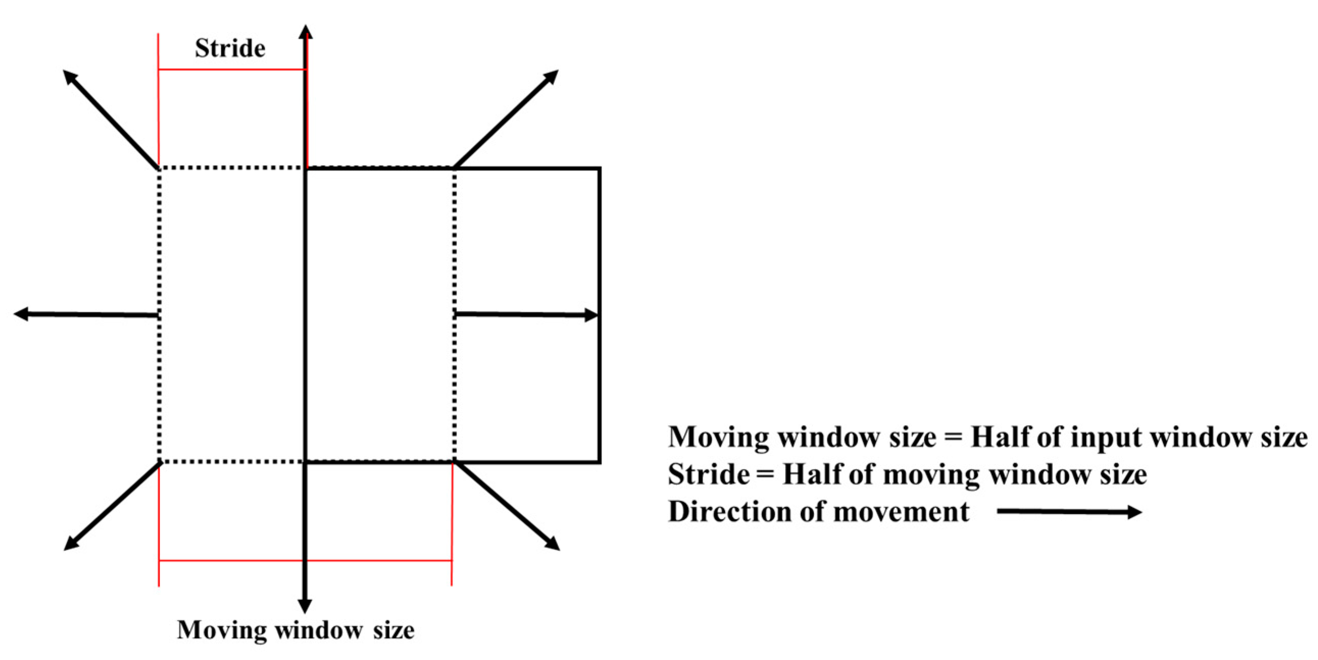
In this study, a random window-moving technique was employed specifically to account for landslide-related factors [31], as shown in the schematic diagram in Figure 5. The implementation details of the random window-moving technique are as follows: the window size was set to half of the input window size, with the stride set to half of the moving window size, ensuring substantial overlap and continuous coverage across the image. Boundary handling was managed through padding, maintaining consistency in feature dimensions across the entire image. Window starting positions were selected entirely at random, increasing the diversity of sampled image segments and potentially increasing the robustness of the model to variations in input data. Additionally, care was taken to ensure that the data was centered within the window, facilitating better capture of local features within the window and improving the model’s recognition ability.
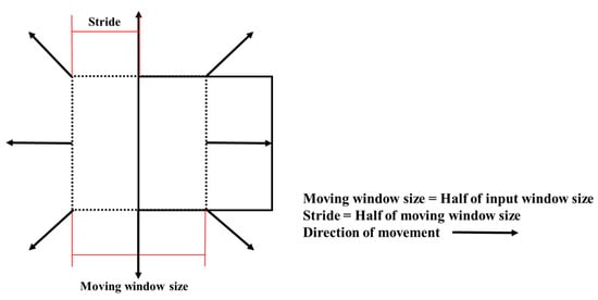
Figure 5.
Schematic diagram of shifting method.
3.4. Evaluation Method
A confusion matrix serves as a tabular representation commonly utilized to evaluate the performance of a classification algorithm. It offers a comprehensive means of assessing the model’s performance by categorizing the predicted and actual classes into four distinct categories. The confusion matrix is conventionally organized as shown in Table 2.

Table 2.
The confusion matrix.
3.4.1. AUC and ROC
Classification models typically output probabilities as predictions, representing the likelihood of belonging to a specific category. For calculating accuracy, these probabilities must be converted into discrete categories, which involves setting a threshold. Probabilities above this threshold are classified into one category, while those below it are classified into another. The choice of threshold directly impacts the accuracy calculation. To address this issue, the Area Under the ROC Curve (AUC) is commonly used.
The AUC is a metric employed to evaluate the performance of binary classification models. The ROC (Receiver Operating Characteristic) curve is a graphical representation illustrating the trade-off between the True Positive Rate and False Positive Rate across various classification thresholds. A higher AUC signifies better discriminative ability in the model, indicating its capability to differentiate between positive and negative instances.
The ROC curve plots the False Positive Rate on the abscissa and the True Positive Rate on the ordinate. The calculation methods for these two indicators are as follows:
3.4.2. Accuracy, Precision, Recall, and the Matthews Correlation Coefficient (MCC)
Accuracy (ACC)
Precision and recall correspond to looking at TP from two different dimensions and the predictive effect of positive examples. Precision is, subjectively, the effect of positive examples being correctly divided; the denominator of precision is (TP + FP), which represents the number of all predicted positive examples. Precision represents the proportion of all positive examples that are actually positive. Precision represents the subjective prediction effect of positive examples. Recall is, objectively, the positive example correctly classified. The denominator of recall is (TP + FN), which represents the number of all actual positive instances. Recall represents the proportion of predictions that are correct among all actual positive examples. Recall indicates whether the prediction effect of the positive example is good or not.
In binary classification tasks, precision (P-score) and recall (R-score) are commonly used to evaluate model effectiveness. Precision measures the accuracy of positive predictions, while recall assesses the ability of the model to identify all relevant instances. However, when these metrics yield divergent results, it complicates the comparison of different models’ performance. For instance, consider two models, A and B: Model A exhibits a higher recall, whereas Model B demonstrates a greater precision. To resolve this dilemma and provide a balanced evaluation, the F-score is employed. This metric integrates precision and recall into a single score, offering a comprehensive measure of a model’s accuracy and completeness. Specifically, the F1 score is used in our analysis, assigning equal importance to both precision and recall, thereby facilitating nuanced comparisons between models where traditional metrics might conflict.
Precision (P-score)
Recall (R-score)
F1-Score (F-score)
In ML, the Matthews correlation coefficient (MCC) has been used as a measure of binary classifications, even if the two classes are of very different sizes [32]. The MCC is defined as follows:
3.4.3. Information Gain Ratio (IGR) Method
In this research, the information gain ratio (IGR) method was employed using the training dataset. A higher IGR value for a landslide causative factor indicates its greater importance to the models. An IGR of zero signifies that a factor contributes nothing to the models and should be excluded [30,33].
4. Results and Discussion
4.1. Importance of Features
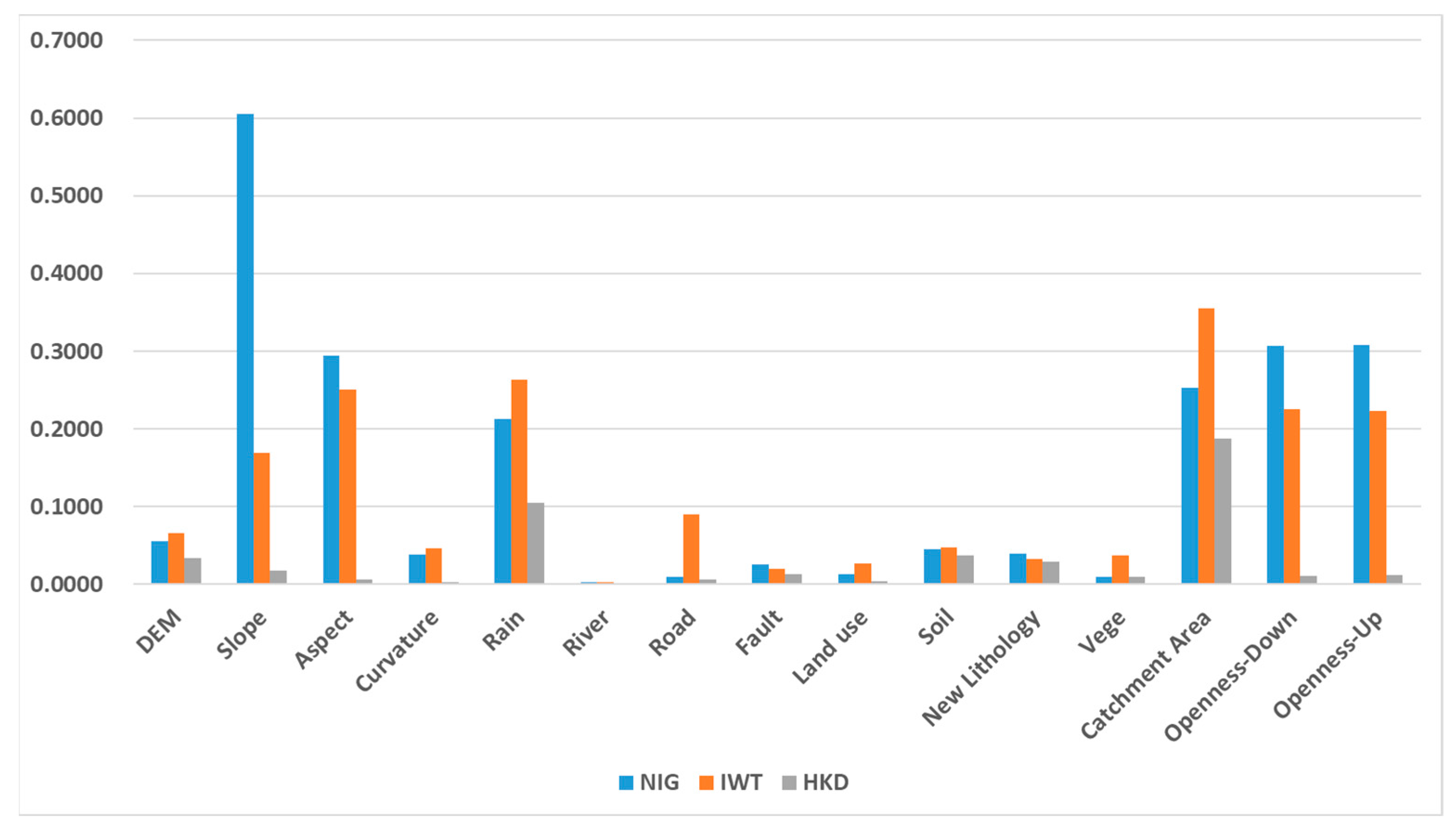
As shown in Figure 6, the IGR values of all 13 factors exceeded zero, indicating their relevance to landslide modeling in our study. Consequently, all selected landslide causative factors were utilized for modeling. However, slight regional variations were observed in IGR values across the three areas. The NIG and IWT regions exhibited similar IGR patterns, while the HKD region showed distinct differences.

Figure 6.
Information gain ratio of the landslide feature.
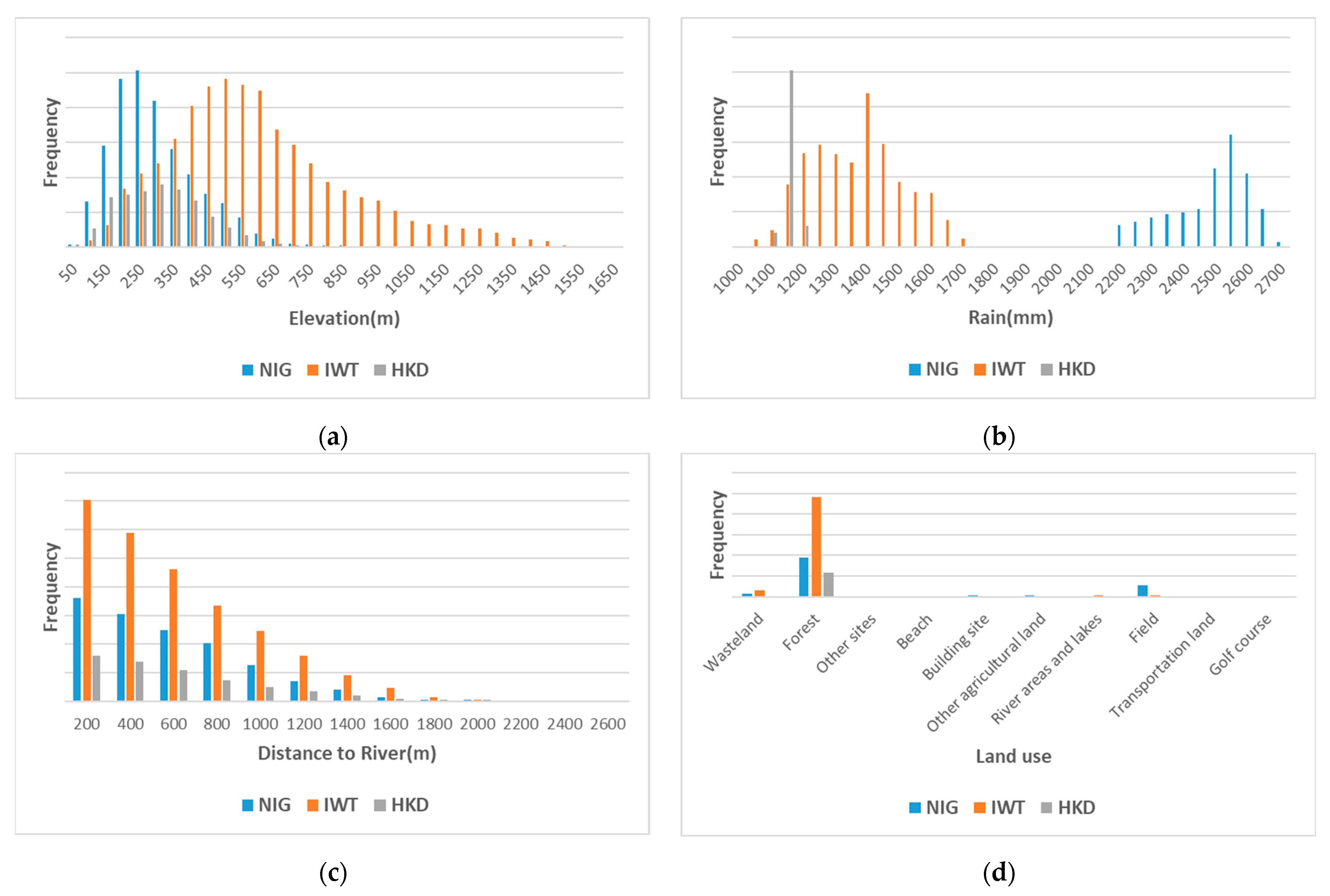
In all study areas, the features with high IGR values primarily included topography and rainfall data, whereas geological data and distance to road, river, and faults had lower IGR values. Compared with geological data, according to the landslide distribution map and feature distribution map, landslides have a larger distribution range of topography and rain data, but the distribution range is smaller in geological data, shown in Figure 7. At the same time, the impact of topography and rain data on landslides is more intuitive. For example, in mountainous areas with high altitudes, large slopes, and dense rainwater, landslides are more likely to occur than in other areas. In the study area, landslides are concentrated in one or few types of soil, land use, and lithology. In the HKD area, all IGR values are smaller than the IWT and NIG areas. The main reason is that the landslides in distribution HKD are concentrated in the upper right part of this area, and the relative number of recorded landslides is far less than those in the other two study areas.
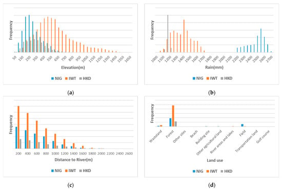
Figure 7.
Distribution frequency of landslides with different features: (a) Elevation, (b) Rainfall, (c) Distance to river, (d) Land use.
4.2. Window Size
4.2.1. Window Size and Landslide Scale
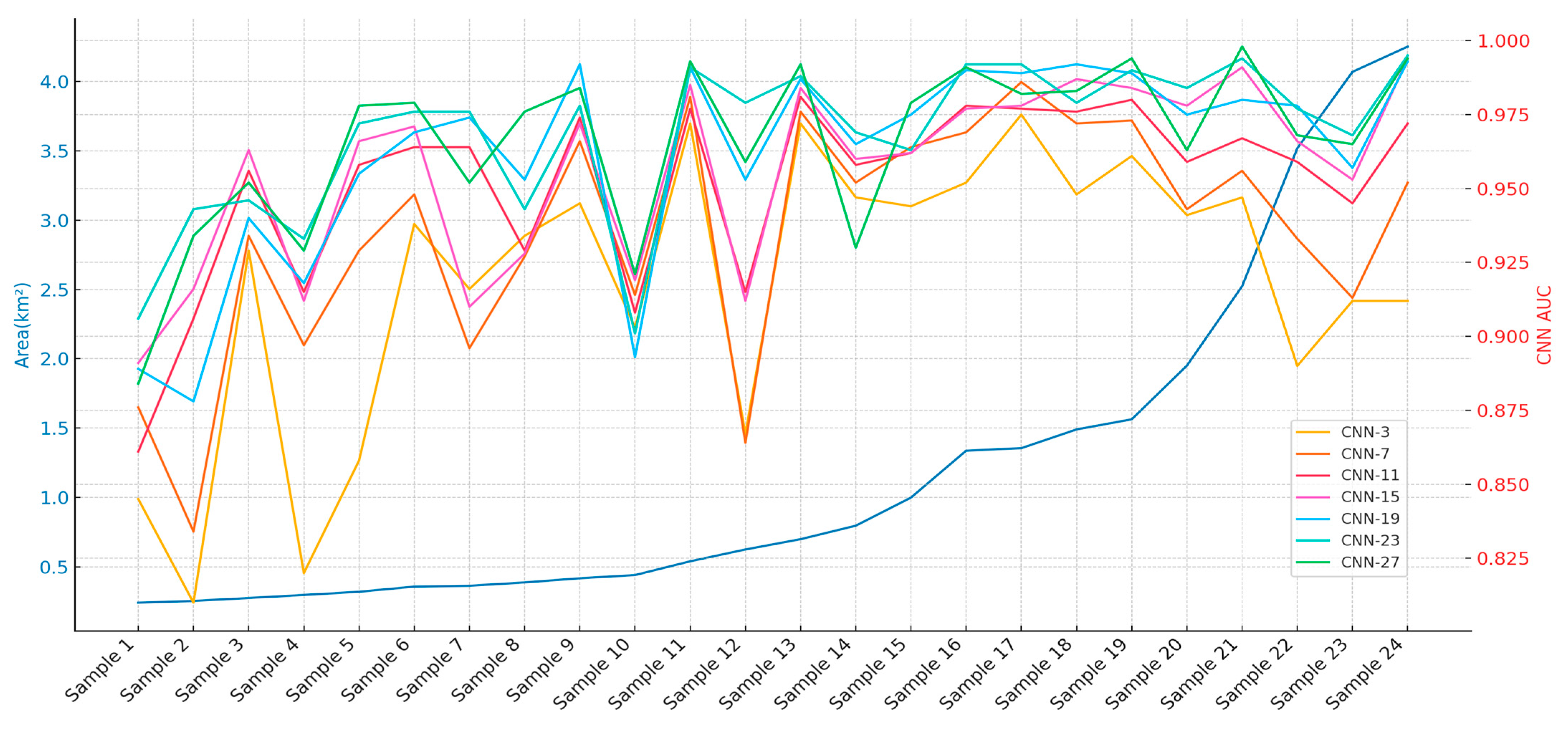
Our study extended the analysis of CNN model performance across different landslide area scales, randomly selecting 24 landslides of different scales with a unified 9 study area in the three study areas of HKD, NIG, and IWT, to study the input window size and landslide scale. The changes in landslide scale and AUC of different CNN-i models are shown in Figure 8.
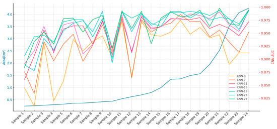
Figure 8.
Variation of landslide areas across landslide scale samples and AUC of CNN-i models across landslide scale.
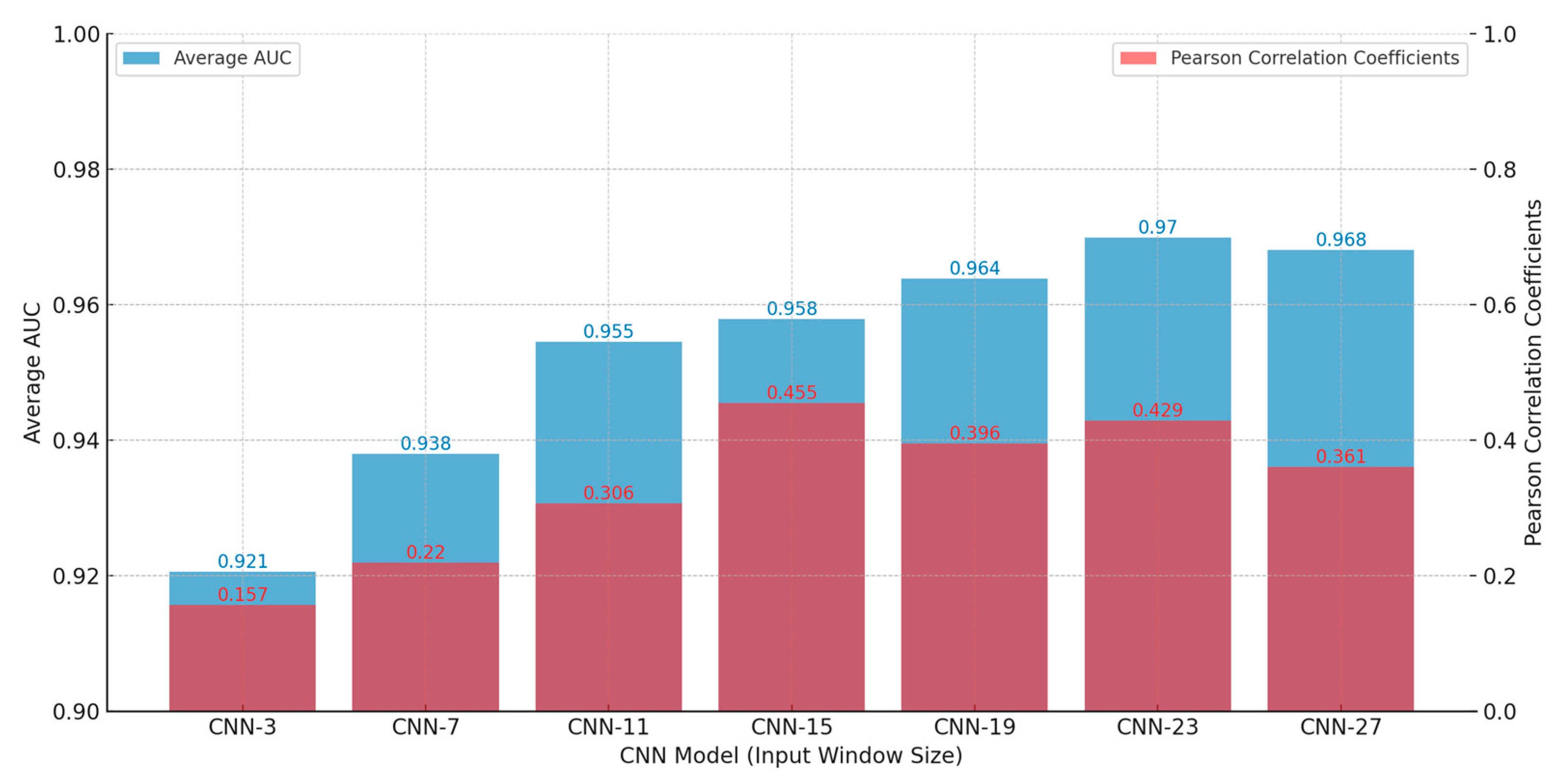
The analysis of CNN models, ranging from CNN-3 to CNN-27, illustrates their effectiveness in predicting landslide scales through a comparison of average AUC values for all samples and Pearson correlation coefficients (as shown in Figure 9). This study emphasizes the crucial role of input window size in determining model accuracy and its correlation with actual landslide dimensions. Models like CNN-19 and CNN-23 stand out, achieving the highest AUC scores, which suggests their strong ability to capture critical features with well-sized input windows. In contrast, the smallest (CNN-3) and largest (CNN-27) window sizes exhibited lower correlation coefficients, likely due to underfitting and overfitting, respectively. The optimal range of window sizes, identified between 15 × 15 and 23 × 23 pixels, strikes a balance by providing sufficient contextual information without introducing excessive noise. This range enhances classification accuracy and maintains strong correlations with real-world landslide data, optimizing both predictive power and model relevance.

Figure 9.
Average AUC and Pearson correlation coefficients of CNN models for landslide scale.
Building on these findings, the decision was made to employ CNN models ranging from CNN-15 to CNN-23 to analyze the entire study area, while also examining the results of CNN-3 to CNN-11 for comparison. Models within the CNN-15 to CNN-23 range, with their medium-sized input windows, are particularly effective at capturing essential landscape features related to landslide scales, thereby ensuring high performance. This effectiveness is reflected in their high average AUC values, indicating strong discriminative capabilities in classifying landslide-prone and non-landslide areas. Among these, CNN-15 stands out, exhibiting the highest Pearson correlation coefficients, which validate a strong linear relationship between the model’s predictions and actual landslide sizes. This correlation is vital because it confirms the models’ capacity to generate results that accurately reflect real-world geological conditions. The adaptability of these models across different terrains further enhances their suitability for broad-scale geographical analyses, making them valuable tools for reliable and precise landslide prediction. This precision is crucial for comprehensive landslide risk assessment and management. By strategically selecting CNN-15 to CNN-23 models, the approach optimizes performance across key metrics, setting the stage for future improvements. This could include hybrid or ensemble methods, which have the potential to further increase both accuracy and applicability in various environmental contexts.
4.2.2. Window Size and Whole Study Area
Based on the results from the trained models for each study area (HKD, NIG, and IWT) using both downsampling and oversampling methods while varying window sizes, the findings confirm that, regardless of the sampling method, increasing the window size leads to improvements in evaluation indices such as AUC, P-score, and R-score. For example, in the HKD region, the trained model’s accuracy improved from 0.907 with a 3 × 3 pixel window size to 0.943 with a 19 × 19 pixel window size. Similarly, the AUC increased from 0.964 to 0.982 (in Table 3 and Table A3). When applied to the test data, the model also demonstrated improvements, with accuracy increasing from 0.887 to 0.913 and the P-score rising from 0.216 to 0.271 as the window size increased (in Table 4 and Table A4). Comparison with results in Table A1 for ACC and AUC from machine learning demonstrates that the CNN model outperforms traditional machine learning approaches across all window sizes, indicating a more robust performance.

Table 3.
(a) Trained CNN-15 to CNN-23 model results with downsampling method. (b) Test group results using trained CNN-15 to CNN-23 models with downsampling method.

Table 4.
(a) Trained CNN-15 to CNN-23 model results with oversampling method. (b) Test group results using trained CNN-15 to CNN-23 models with oversampling method.
Larger window sizes allow the model to capture a wider range of environmental variables simultaneously, enabling it to understand more complex interactions. For example, larger windows can incorporate diverse topographical gradients, soil types, and hydrological features that smaller windows may overlook, leading to a more detailed comprehension of landslide triggers. By offering a broader spatial context, CNN models can distinguish more effectively between landslide-prone and stable areas. This is particularly advantageous in complex terrains where local conditions may not fully represent regional dynamics, and larger windows provide a macroscopic view that helps in identifying patterns indicating instability.
Among the various CNN configurations tested, CNN-19 emerges as the best model for predicting landslide scales, outperforming models like CNN-15 and CNN-23. CNN-19’s 19 × 19 input window strikes an ideal balance—large enough to include essential terrain features for accurate landslide modeling, yet small enough to avoid incorporating irrelevant data that could lower performance. This optimal window size allows CNN-19 to capture a comprehensive landscape view while maintaining generalization across diverse terrains without the underfitting or overfitting issues associated with smaller (CNN-15) or larger (CNN-23) windows.
In addition to high AUC values, CNN-19 maintains strong Pearson correlation coefficients, ensuring that its predictions not only effectively classify landslide-prone areas but also align closely with actual landslide dimensions, reflecting a reliable geological understanding. While CNN-15 may be underfit in complex terrains due to its smaller window, and CNN-23 may be overfit by incorporating excessive noise, CNN-19 strikes the right balance, making it the most effective in capturing the dynamics of landslides.
However, larger window sizes come with challenges, such as increased computational demand and higher memory requirements, which can limit real-time application. Additionally, the resolution of the input data is critical for selecting the optimal window size. Future research could explore multi-scale analysis, training models with different window sizes to improve robustness, or integrating CNNs with other machine learning methods to mitigate the limitations of single-scale models, potentially resulting in more accurate landslide prediction systems.
Furthermore, the inherent imbalance in the test data structure may lead to a disparity between the test and trained model results, with test results often underperforming compared to the trained models.
4.3. Sampling Method
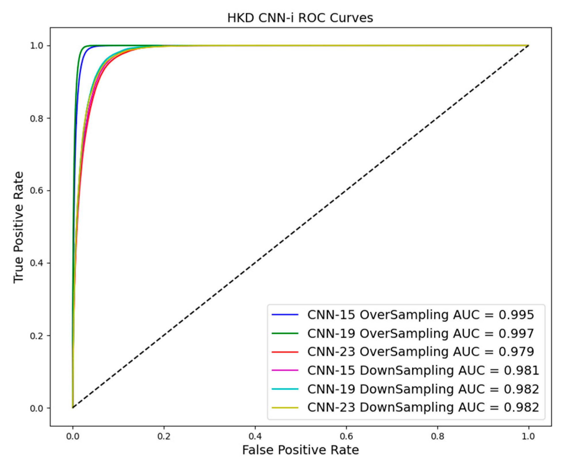
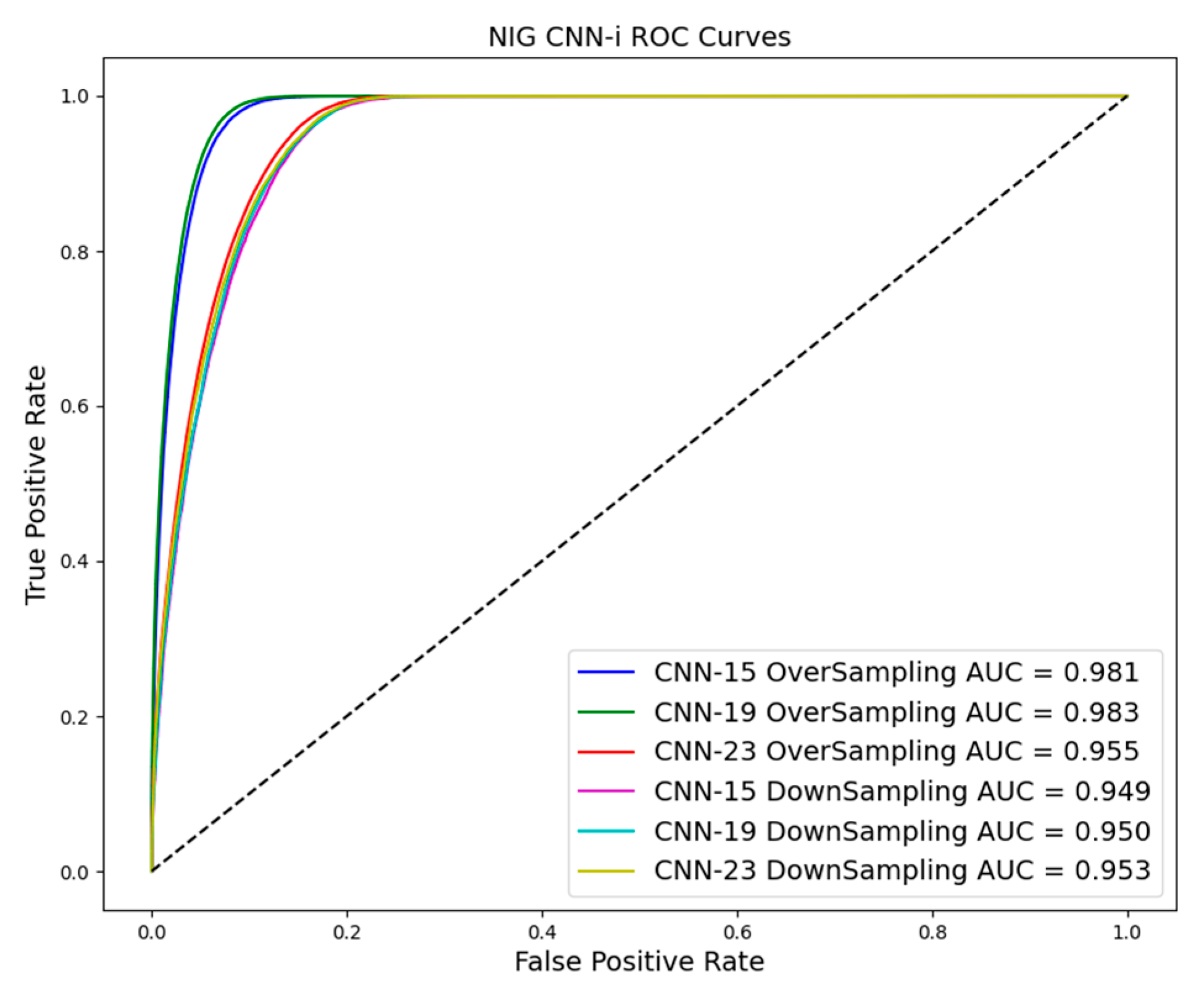
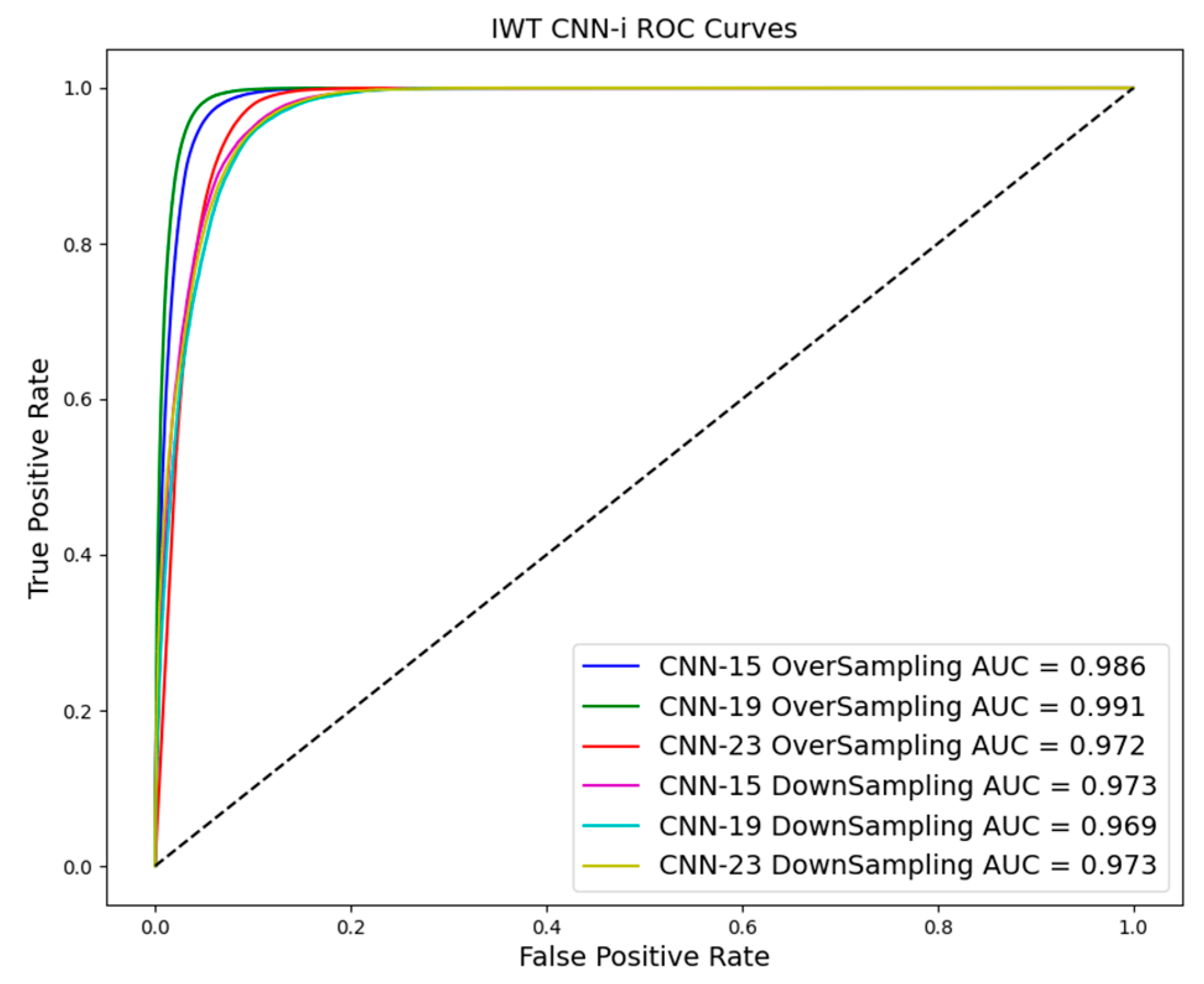
As shown in Table 3 and Table 4 and Figure 10, Figure 11 and Figure 12, evaluation indices such as AUC, P-score, and R-score obtained from models trained using the oversampling method tend to be higher than those using the downsampling method. This improvement is evident in both training and test results.
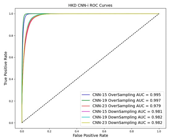
Figure 10.
ROC curve in downsampling and oversampling in HKD based on CNN-i.
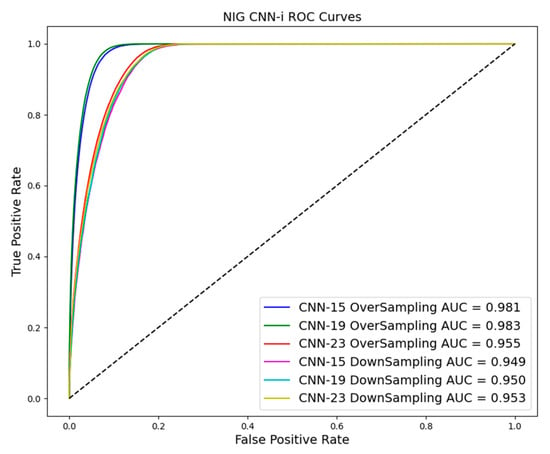
Figure 11.
ROC curve in downsampling and oversampling in NIG based on CNN-i.
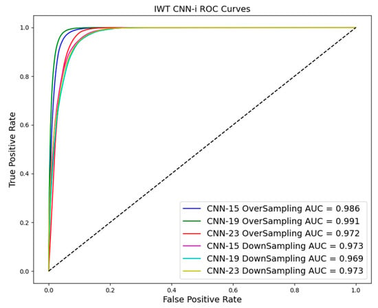
Figure 12.
ROC curve in downsampling and oversampling in IWT based on CNN-i.
The superiority of oversampling is particularly pronounced in the test model, where it outperforms the downsampling technique. Firstly, oversampling increases the number of samples across the entire dataset, which is crucial for training CNN models. Secondly, the oversampled data in this study consist of landslide data samples, making them distinct from non-landslide data. Achieving data alignment and sample balance is essential in deep learning, and oversampling effectively addresses these concerns.
As a result, oversampling increases the representation of landslide instances in the training data, significantly enhancing the model’s ability to detect subtle cues associated with landslide occurrences. This method reduces the model’s bias towards the more frequent non-landslide class. However, it may also introduce variance by potentially overfitting to the landslide class, particularly if the oversampling technique simply replicates existing samples without introducing variability.
On the other hand, while downsampling helps balance the classes by reducing the size of the dominant non-landslide class, it risks losing valuable information critical for identifying landslides. This approach can inadvertently simplify the model’s view of the landscape, potentially leading to underfitting and poorer generalization on new, unseen data.
In summary, both oversampling and downsampling have certain drawbacks. Further research should investigate adaptive sampling techniques that dynamically adjust the sampling method based on real-time model performance and feedback. This approach could optimize the balance between bias and variance dynamically, improving model accuracy and generalizability. Additionally, exploring advanced oversampling techniques that introduce more realistic variability into the training data could help develop more robust and accurate landslide prediction models.
4.4. Visualization
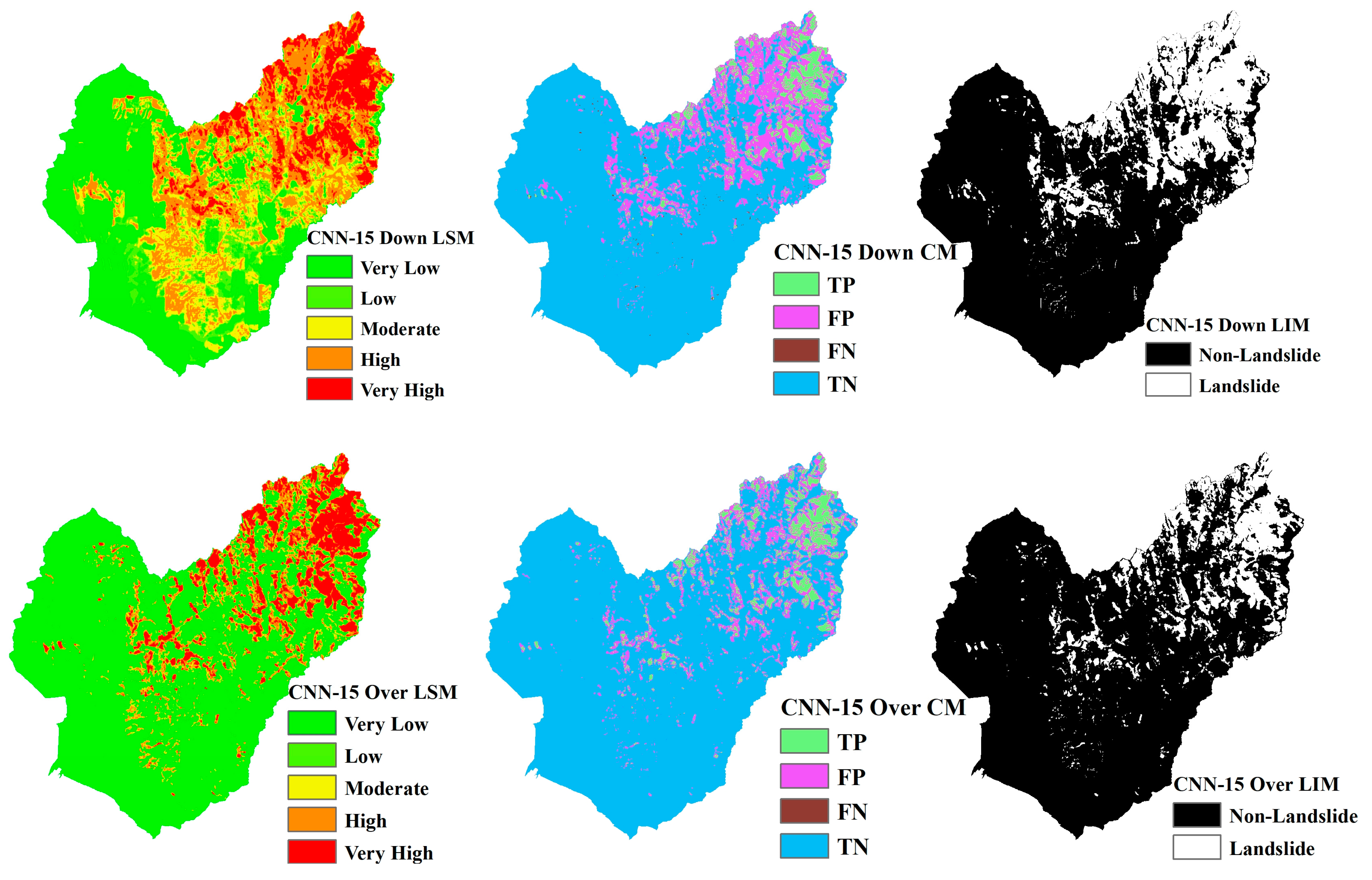
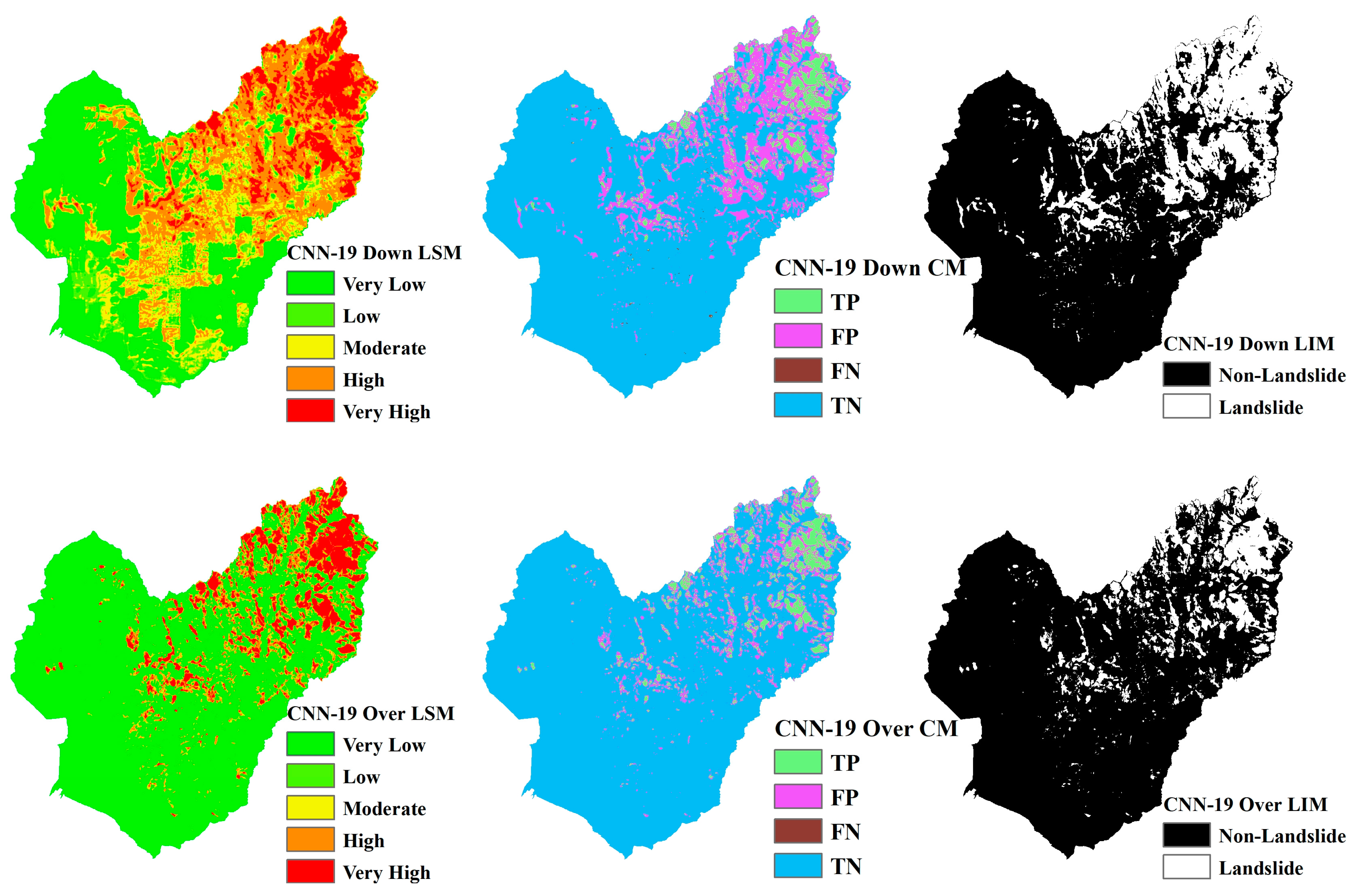
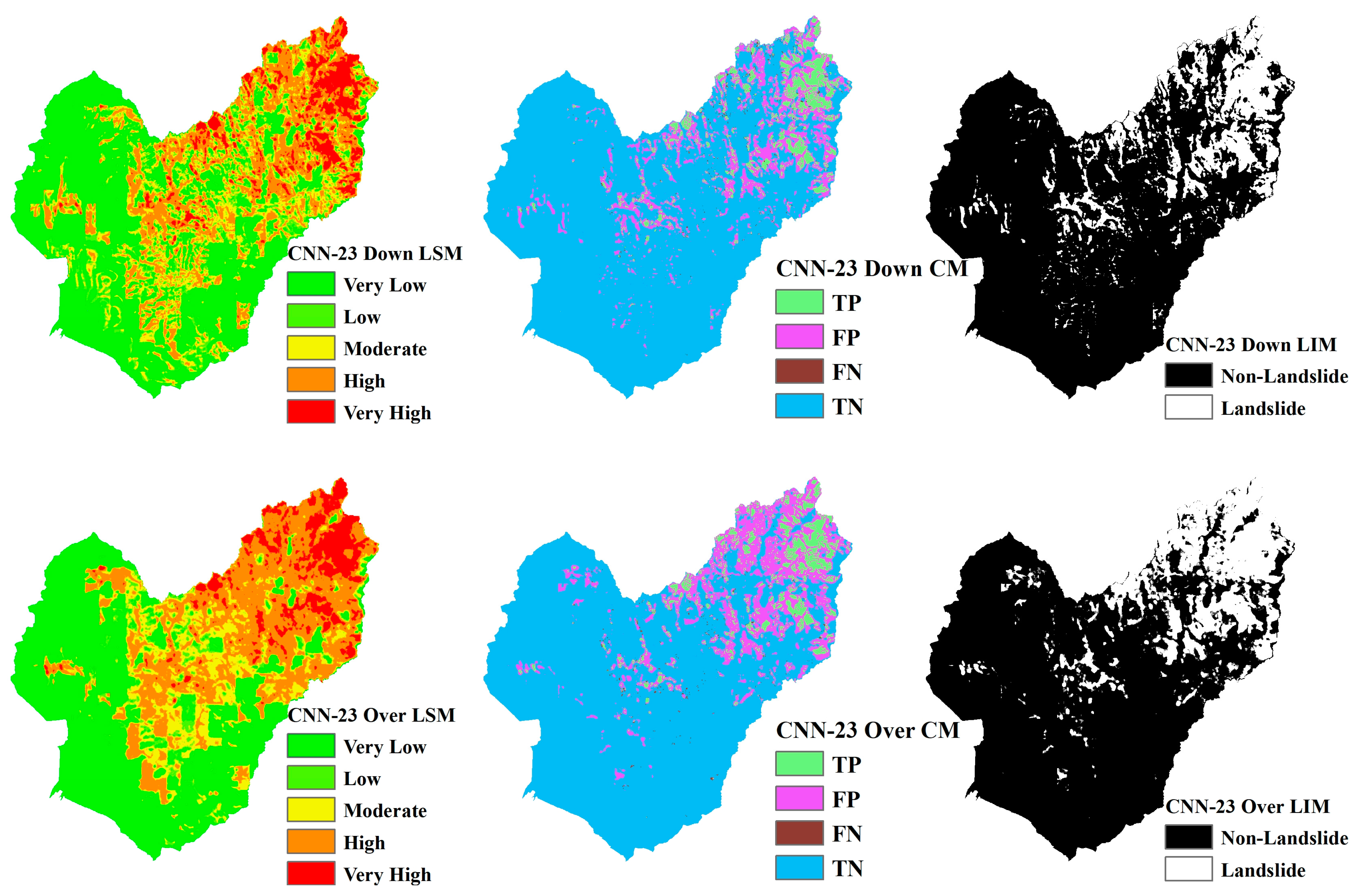
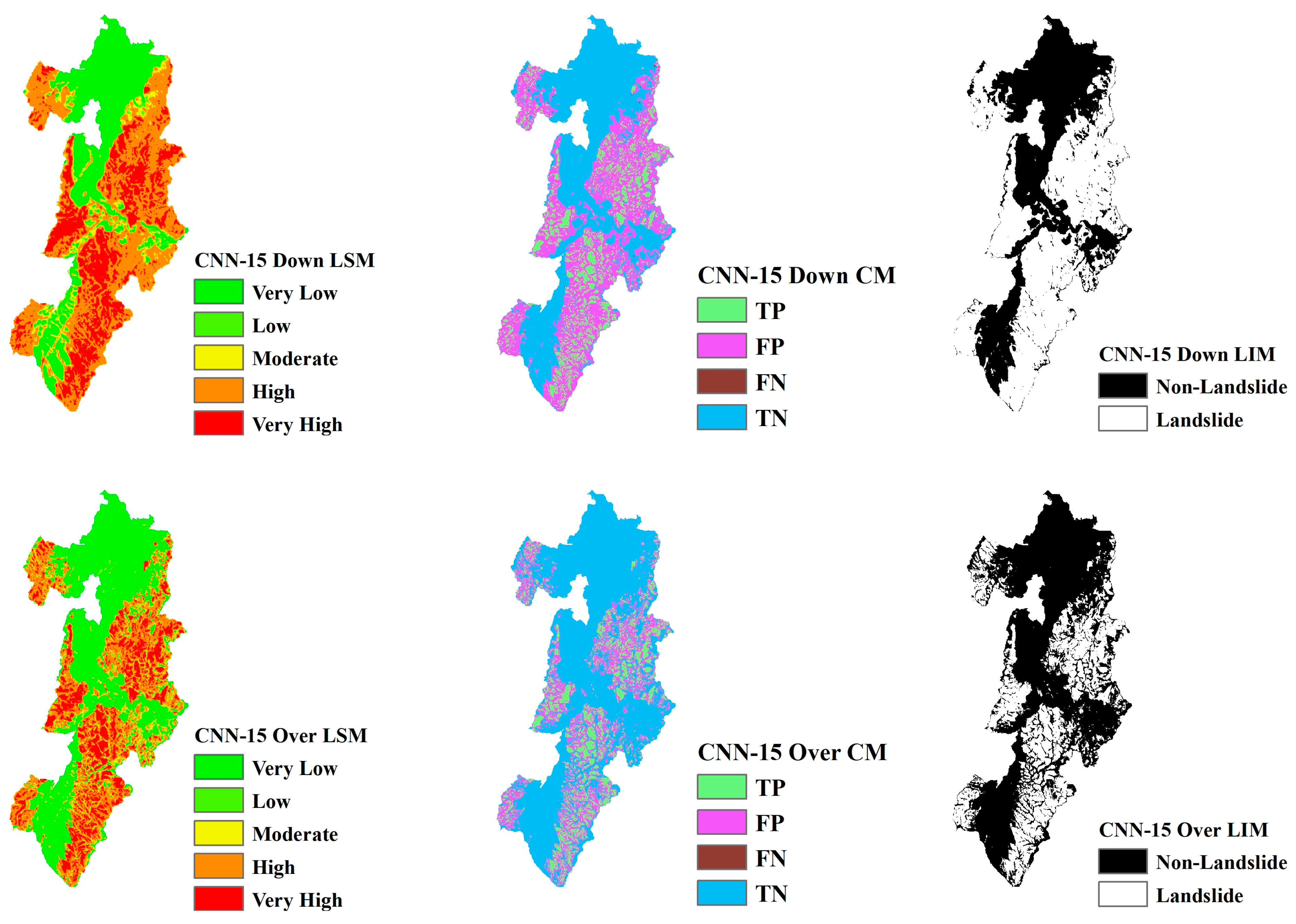
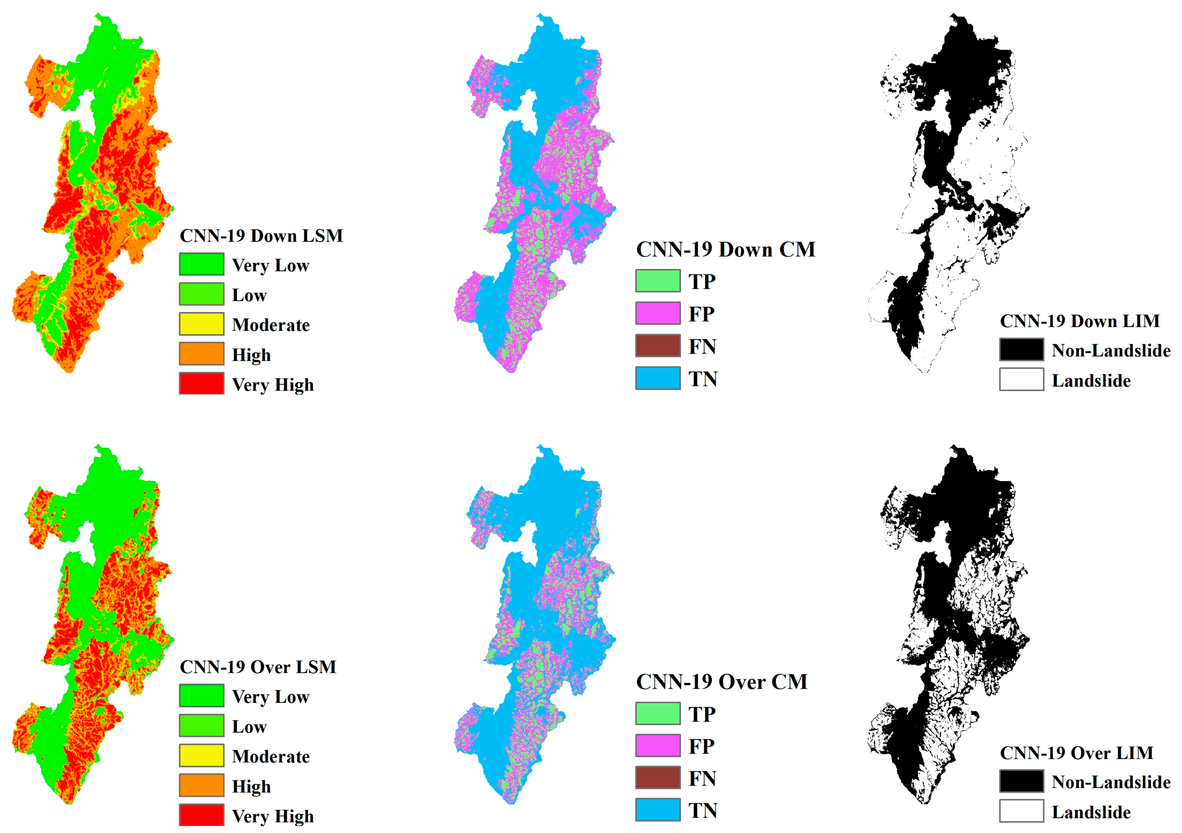
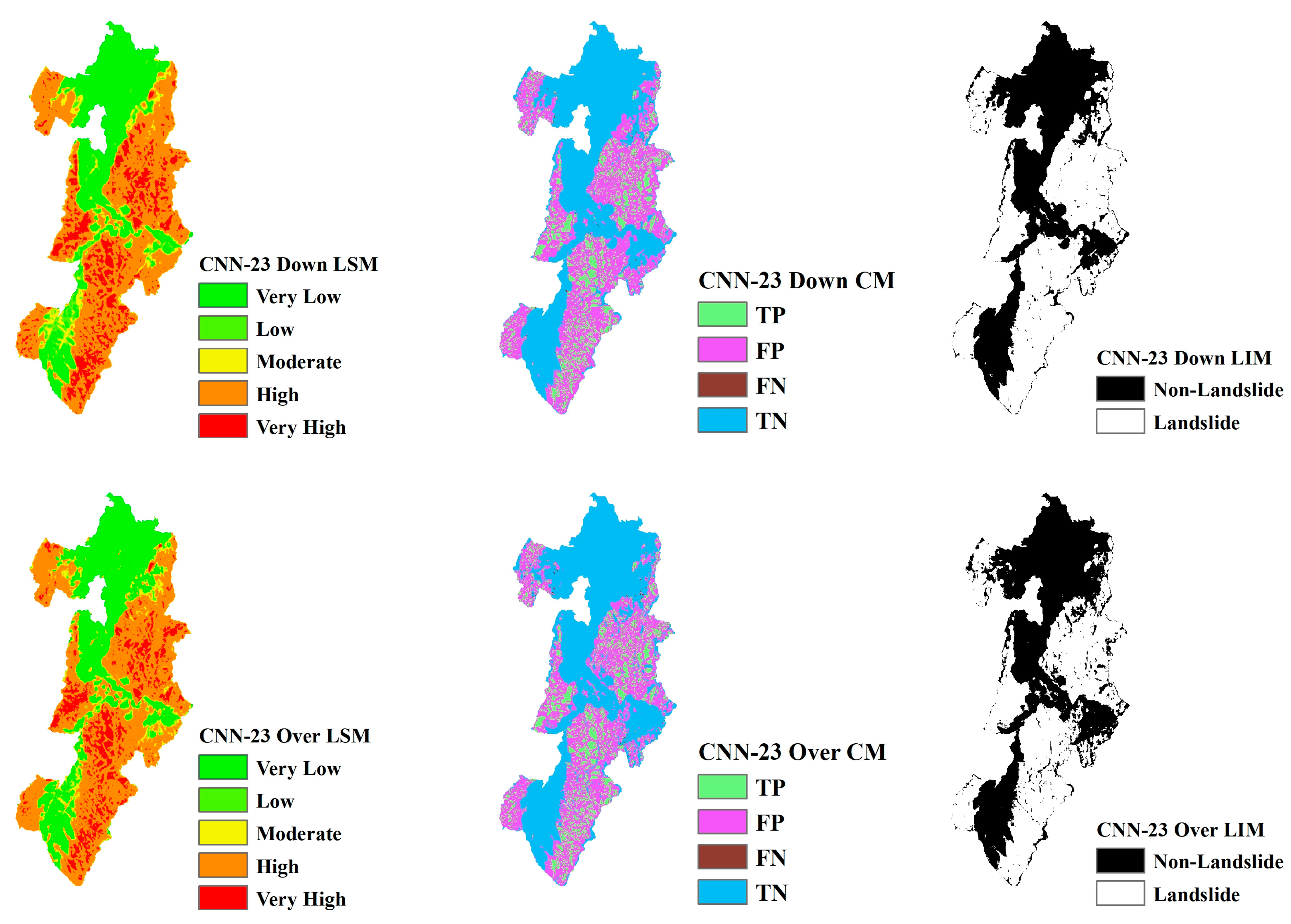
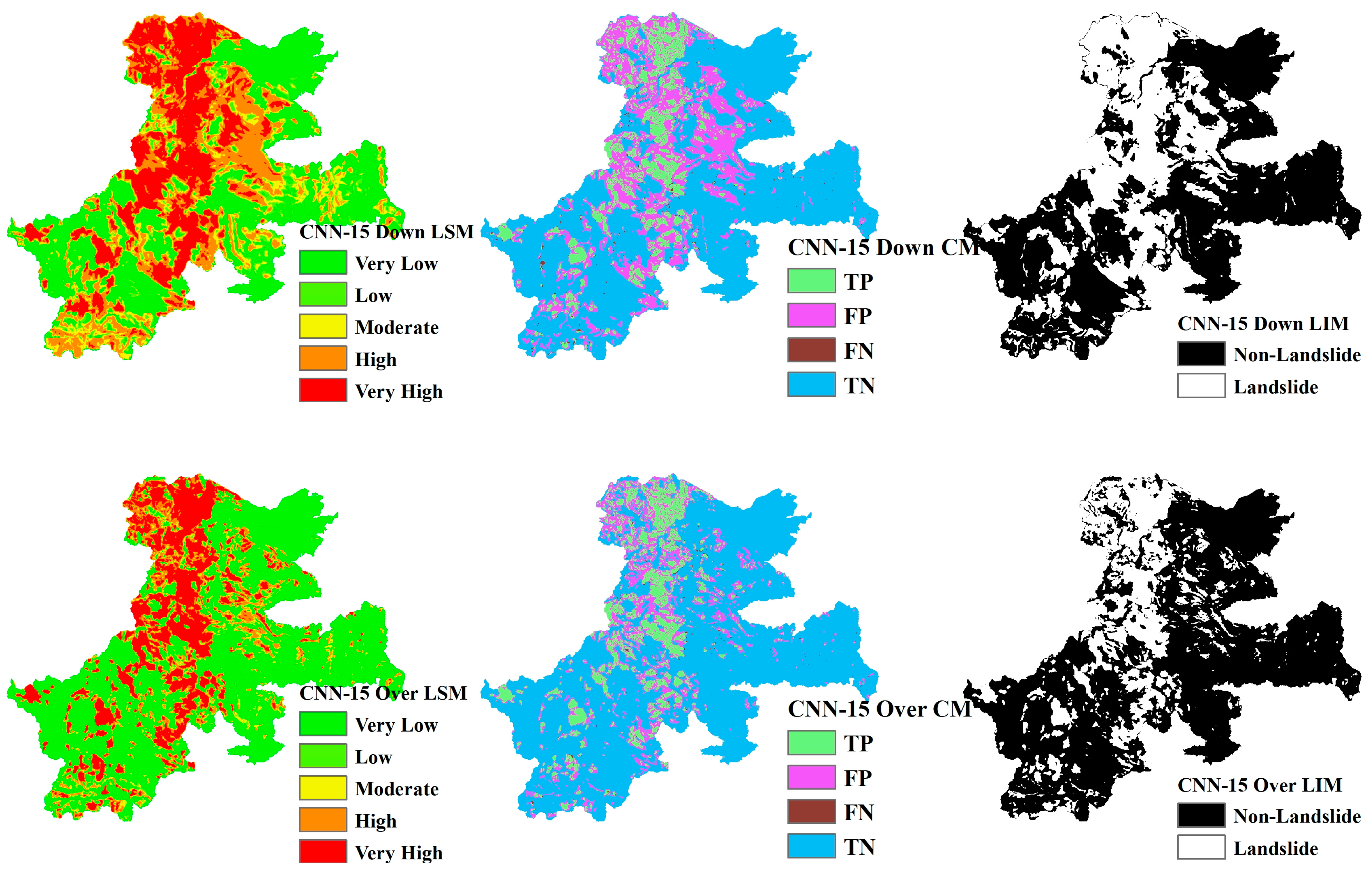
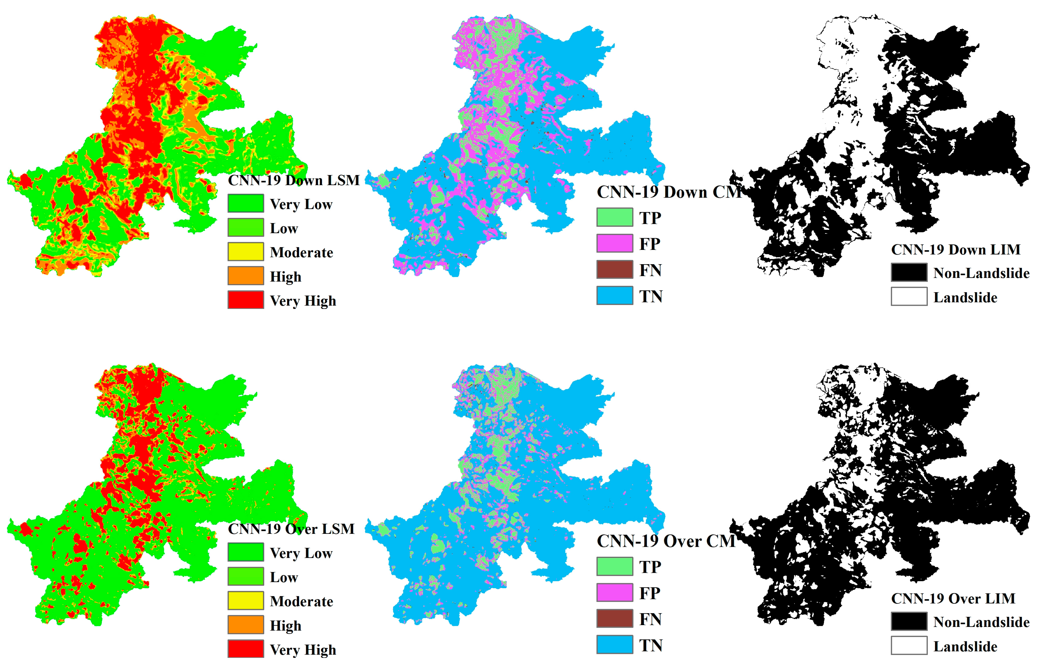
Landslide Susceptibility Mapping (LSM), Landslide Inventory Mapping (LIM), and the confusion matrix (CM) based on CNN models ranging from CNN-15 to CNN-23 are shown in Figure 13, Figure 14, Figure 15, Figure 16, Figure 17, Figure 18, Figure 19, Figure 20 and Figure 21. The LSM categorizes landslide risk into five levels: very low, low, moderate, high, and very high, enabling precise risk assessment across various geographic regions. LIM, on the other hand, uses the outcomes from the trained CNN models to test and predict the original dataset. The key difference between LSM and LIM is that LSM assesses potential hazard levels, while LIM focuses on the detection of actual landslide events. The confusion matrix (CM) visualization further provides a detailed analysis of the model’s performance, giving insights into accuracy, recall, precision, and misclassification rates within each category. This helps to identify both the model’s strengths and areas where the model needs improvement.
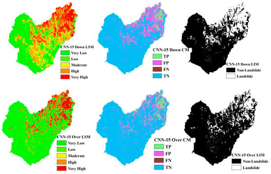
Figure 13.
LSM, CM, and LIM in CNN-15 (upper: downsampling, lower: oversampling).

Figure 14.
LSM, CM, and LIM of HKD in CNN-19 (upper: downsampling, lower: oversampling).
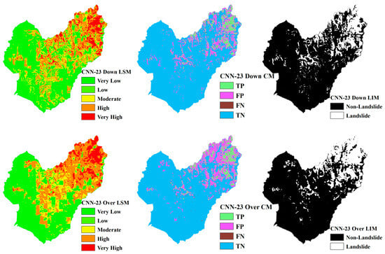
Figure 15.
LSM, CM, and LIM of HKD in CNN-23 (upper: downsampling, lower: oversampling).
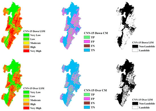
Figure 16.
LSM, CM, and LIM of NIG in CNN-15 (upper: downsampling, lower: oversampling).
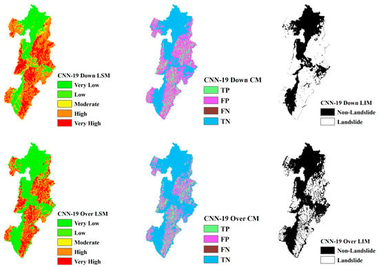
Figure 17.
LSM, CM, and LIM of NIG in CNN-19 (upper: downsampling, lower: oversampling).
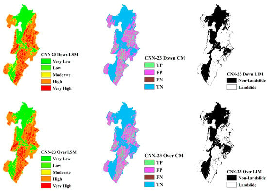
Figure 18.
LSM, CM, and LIM of NIG in CNN-23 (upper: downsampling, lower: oversampling).
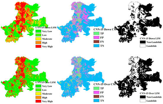
Figure 19.
LSM, CM, and LIM of IWT in CNN-15 (upper: downsampling, lower: oversampling).
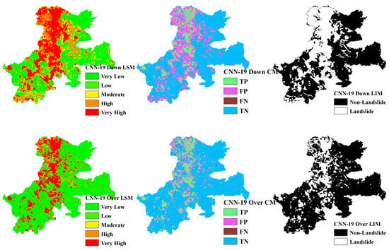
Figure 20.
LSM, CM, and LIM of IWT in CNN-19 (upper: downsampling, lower: oversampling).
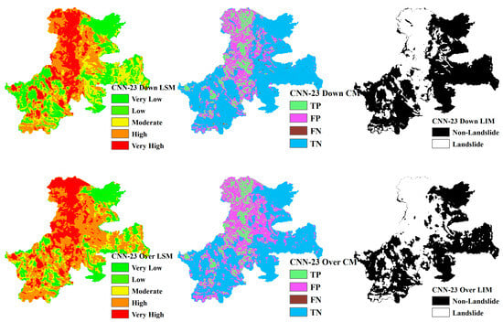
Figure 21.
LSM, CM, and LIM of IWT in CNN-23 (upper: downsampling, lower: oversampling).
Across different study areas, CNN-19 stands out, outperforming both CNN-15 and CNN-23 in terms of accuracy and predictive reliability, particularly when paired with sophisticated sampling techniques.
4.5. Versatility
The accuracy and confusion matrix of the results shown in Table 5 was obtained by applying the CNN models trained on data from one study area to test data from a different study area. These results indicate that using HKD as the training area produces better outcomes than when NIG or IWT are used as training regions. Similarly, when evaluated based on R-score and AUC, training on HKD achieves higher performance. Additionally, LSM corroborates these findings, as depicted in Figure 22, Figure 23 and Figure 24. Although accuracy alone does not fully confirm the proposed CNN model’s versatility, the obtained results are generally acceptable, given the substantial amount of non-landslide data.

Table 5.
Different test area results based on different area-trained CNN-19 model with oversampling.

Figure 22.
CM based on the CNN-19 with the oversampling method in HKD. Left to right: IWT, HKD, and NIG.

Figure 23.
CM based on the CNN-19 with the oversampling method in NIG. Left to right: IWT, HKD, and NIG.

Figure 24.
CM based on the CNN-19 with the oversampling method in IWT. Left to right: IWT, HKD, and NIG.
Analysis of the Information Gain Ratio (IGR) results suggest a possible explanation for the notable differences observed between the HKD and the NIG and IWT regions. In the HKD area, no single feature exhibits significant influence, whereas in the NIG and IWT regions, certain features demonstrate a significantly higher influence compared to others, leading to pronounced regional characteristics. Consequently, the model is influenced by these regional characteristics during the training process. However, such strong regional characteristics are absent in the HKD area. Therefore, when the HKD area is used as the training area, the model’s performance when applied to other areas is generally better compared to when the NIG and IWT areas are used as training areas. The variation in IGR among different features across regions suggests that certain features are more influential in some areas than in others. This disparity implies that a model’s ability to generalize across regions can be enhanced by identifying and focusing on features that offer the most predictive power universally, rather than those that are region-specific.
Based on the versatility tests conducted in this research, it must be acknowledged that there are significant challenges in achieving versatility. However, the results also point to specific directions for future efforts. To improve the universality of models, two key aspects must be prioritized. Firstly, when selecting features, it is crucial to avoid those with strong regional characteristics, as these can limit the model’s applicability across different contexts. Secondly, during the model training and testing processes, it is essential to select appropriate sampling methods and model structures. This ensures the development of robust models that are universally applicable. Despite these focused efforts, it is important to recognize that achieving high-precision generalization with the current models remains a challenging task. Therefore, continued research and refinement of models are necessary to enhance their predictive accuracy and generalizability. Additionally, at the current stage, a practical approach remains to assess landslide risks based on specific regional historical landslide records and characteristics. This method leverages localized knowledge and data, allowing for more targeted and effective risk assessment and the potential for proactive landslide mitigation strategies.
5. Conclusions
This study extensively explores the effectiveness of convolutional neural network (CNN) models in landslide risk assessment across three distinct regions, employing various evaluation metrics to assess predictive accuracy, model adaptability, and the impact of regional characteristics and sampling techniques on model performance.
The analysis reveals that increasing the CNN window size significantly improves the model’s predictive capabilities by more comprehensively capturing environmental features, crucial for accurately predicting landslide occurrences. The generalizability of CNN-19 across diverse geographical settings further underscores its suitability for comprehensive analysis across extensive study areas. It adapts well to different environmental conditions, ensuring consistency in predictive performance and reliability. The strategic selection of CNN-19 for landslide scale analysis leverages its capabilities to optimize performance on critical metrics, making it the most appropriate model for such applications. Its ability to balance feature capture with accurate and relevant output makes it a pivotal tool for landslide risk assessment and management, potentially guiding future enhancements and the exploration of hybrid or ensemble models to elevate accuracy and applicability in varied environmental settings. However, the study observes a significant performance disparity between the training and test models, largely due to data imbalances within the test datasets. This discrepancy is more pronounced in scenarios where there is a considerable gap between the number of landslide and non-landslide data points in the original dataset. To address these imbalances, our comparative analysis of downsampling and oversampling techniques demonstrates that oversampling notably enhances model performance in the test sets. This method proves particularly beneficial in imbalanced scenarios, improving model accuracy and overall effectiveness by providing a more balanced representation of both landslide and non-landslide conditions.
Regarding model versatility, the study explores the implications of varying window sizes, sampling methods, and regional feature sensitivities as reflected in Information Gain Ratio (IGR) findings. The results underscore the importance of considering regional characteristics in model training to enhance adaptability and generalizability across different landscapes. Oversampling emerges as a strategic approach to overcome data scarcity and imbalance challenges, significantly contributing to the development of robust models capable of delivering reliable predictions across diverse environmental settings.
Future research should explore advanced machine learning algorithms like Generative Adversarial Networks (GANs) and Recurrent Neural Networks (RNNs) to further enhance model robustness and accuracy. An in-depth examination of the influence of various environmental features on landslide predictions and optimizing feature engineering are vital steps. Additionally, increasing the generalizability of models across regions with varied geological and climatic conditions, and integrating CNN models into real-time disaster monitoring systems, will improve adaptability and practicality. To further enhance this approach, adopting more flexible CNN models and sampling methods is essential. For instance, combining CNN models with different window sizes can be particularly effective. The selection of appropriate sampling methods should be based on the actual conditions of the data, allowing for region-specific adaptations. Not only does this approach tailor the solution to the environmental context, but it also optimizes computational costs. These initiatives are crucial for developing robust models that deliver reliable predictions in diverse environments, thereby advancing disaster risk management and mitigation practices.
Author Contributions
Conceptualization, F.R. and K.I.; methodology, F.R.; software, F.R. and K.I.; validation, F.R.; formal analysis, F.R.; investigation, F.R.; resources, F.R. and K.I.; data curation, F.R.; writing—original draft preparation, F.R.; writing—review and editing, K.I.; visualization, F.R.; supervision, K.I. All authors have read and agreed to the published version of the manuscript.
Funding
This work was partially supported by JST SPRING Grant Number JPMJSP2119, KAKENHI Grant Number 23K04019, and Sato Kogyo Co., Ltd.
Data Availability Statement
The original contributions presented in the study are included in the article, further inquiries can be directed to the corresponding author.
Conflicts of Interest
The authors declare that this study received funding from Sato Kogyo Co., Ltd. The funder was not involved in the study design, collection, analysis, interpretation of data, the writing of this article or the decision to submit it for publication.
Appendix A

Figure A1.
Maps showing parts of landslide features in NIG area: (a) Land use, (b) Soil, (c) Lithology, and (d) Vegetation.
Figure A1.
Maps showing parts of landslide features in NIG area: (a) Land use, (b) Soil, (c) Lithology, and (d) Vegetation.
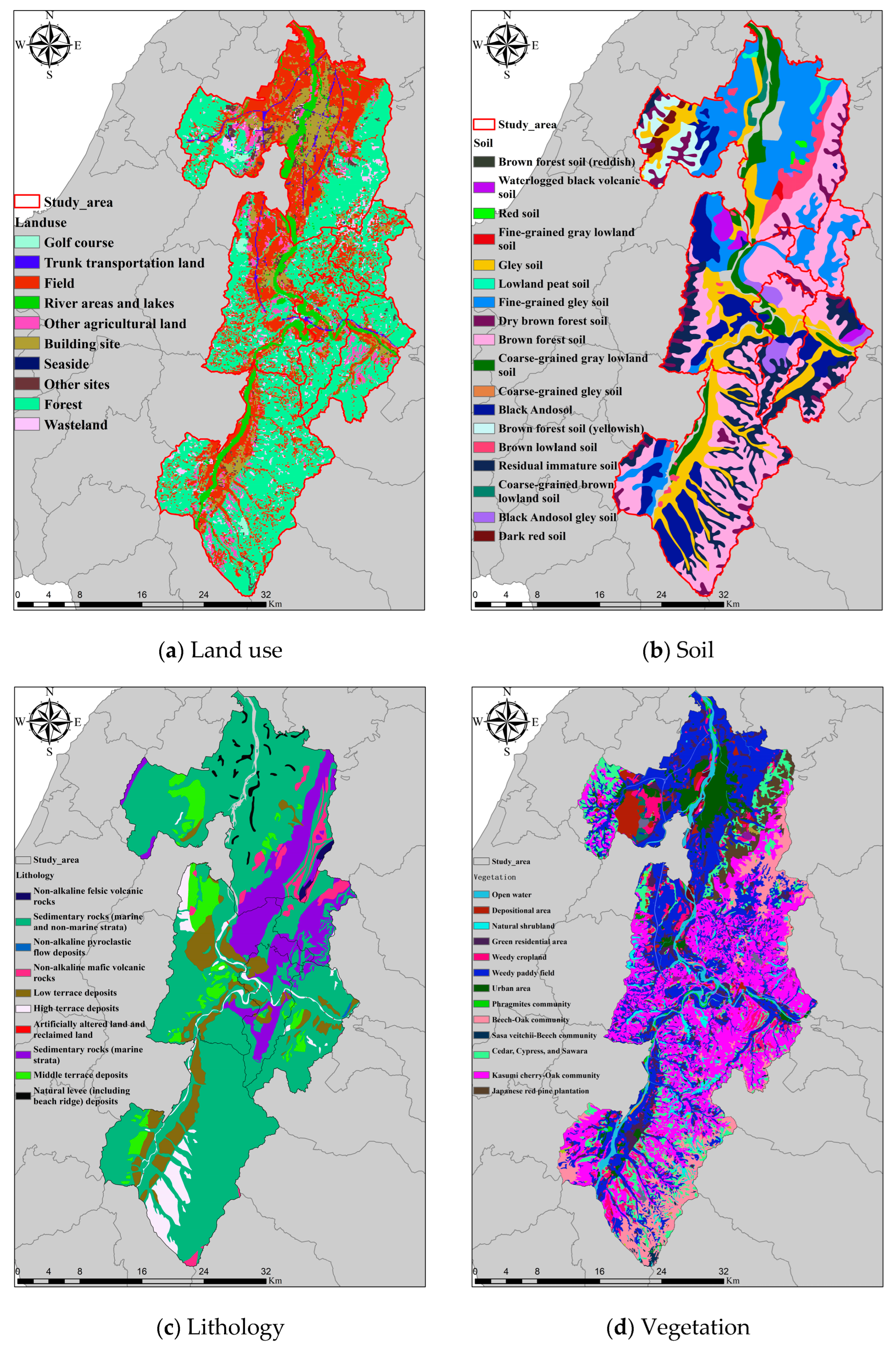
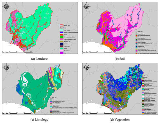
Figure A2.
Maps showing parts of landslide features in HKD area: (a) Land use, (b) Soil, (c) Lithology, and (d) Vegetation.
Figure A2.
Maps showing parts of landslide features in HKD area: (a) Land use, (b) Soil, (c) Lithology, and (d) Vegetation.
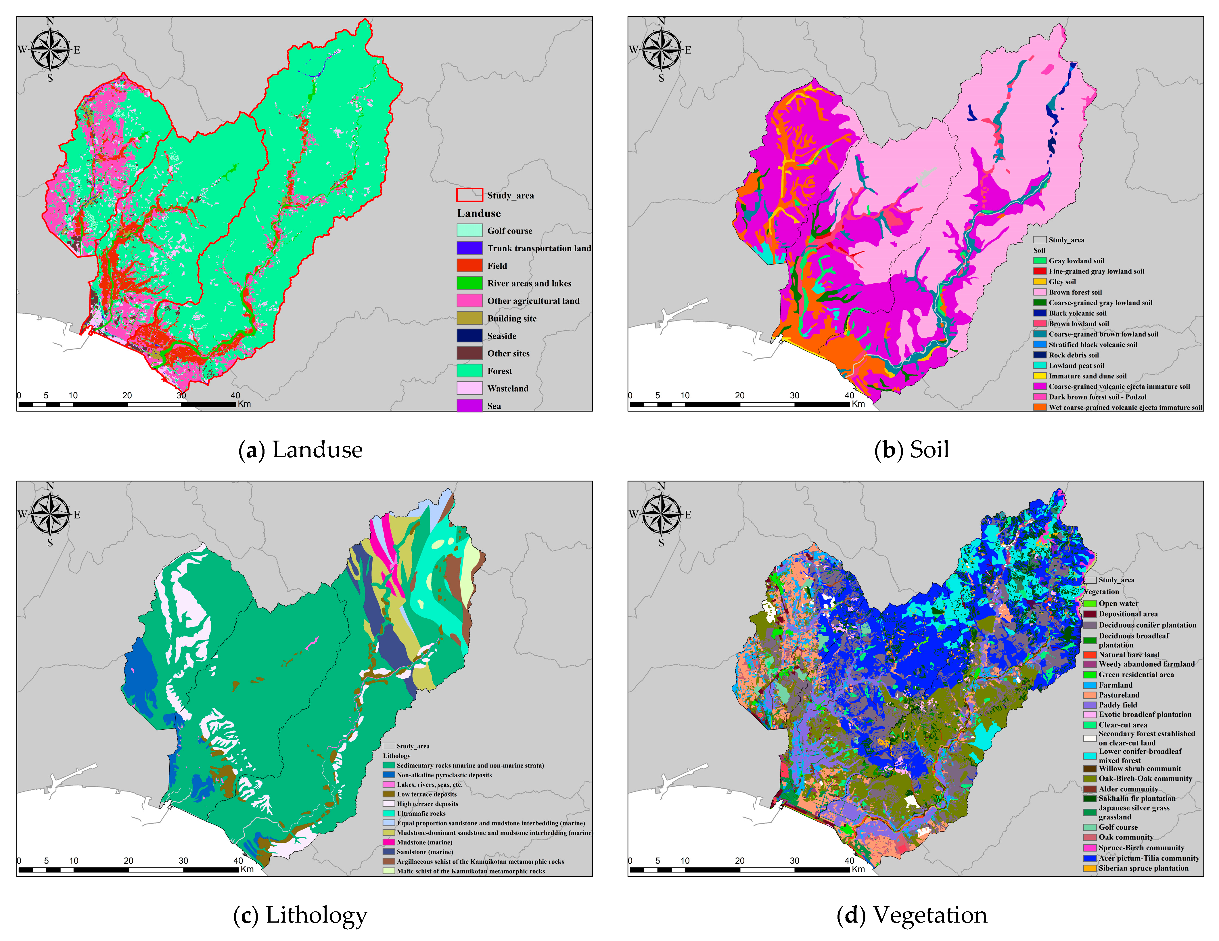

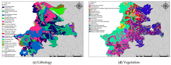
Figure A3.
Maps showing parts of landslide features in IWT-MYG area: (a) Land use, (b) Soil, (c) Lithology, and (d) Vegetation.
Figure A3.
Maps showing parts of landslide features in IWT-MYG area: (a) Land use, (b) Soil, (c) Lithology, and (d) Vegetation.
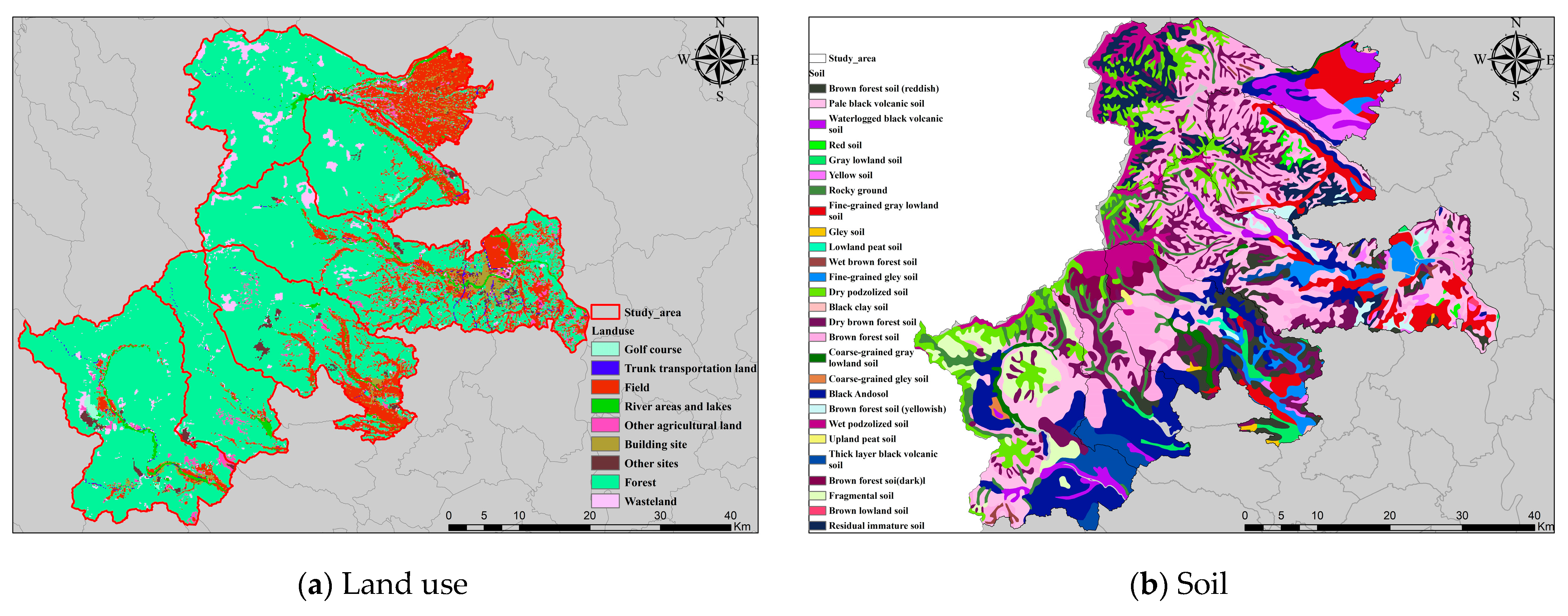


Table A1.
Results obtained by machine learning in three study areas.
Table A1.
Results obtained by machine learning in three study areas.
| Area | LR | DT | RF | KNN | ANN | MLP | |
|---|---|---|---|---|---|---|---|
| NIG | ACC | 0.704 | 0.873 | 0.654 | 0.832 | 0.827 | 0.811 |
| AUC | 0.744 | 0.873 | 0.654 | 0.931 | 0.919 | 0.914 | |
| HKD | ACC | 0.873 | 0.952 | 0.726 | 0.912 | 0.913 | 0.898 |
| AUC | 0.873 | 0.952 | 0.839 | 0.967 | 0.969 | 0.958 | |
| IWT | ACC | 0.802 | 0.908 | 0.756 | 0.848 | 0.880 | 0.876 |
| AUC | 0.769 | 0.961 | 0.844 | 0.927 | 0.938 | 0.942 |

Table A2.
Trained CNN-3 to CNN-11 model results with downsampling method.
Table A2.
Trained CNN-3 to CNN-11 model results with downsampling method.
| Train Area | Model | Confusion Matrix | ACC | P-Score | R-Score | F-Score | AUC | |||
|---|---|---|---|---|---|---|---|---|---|---|
| TP | FP | TN | FN | |||||||
| HKD (Down) | CNN-3 | 45,835 | 5759 | 43,881 | 3437 | 0.907 | 0.888 | 0.930 | 0.909 | 0.964 |
| CNN-7 | 47,525 | 5837 | 43,744 | 1806 | 0.923 | 0.891 | 0.963 | 0.926 | 0.971 | |
| CNN-11 | 47,170 | 4520 | 44,981 | 2241 | 0.932 | 0.913 | 0.955 | 0.933 | 0.977 | |
| NIG (Down) | CNN-3 | 46,111 | 10,928 | 36,115 | 979 | 0.874 | 0.808 | 0.979 | 0.886 | 0.933 |
| CNN-7 | 46,364 | 10,302 | 36,799 | 668 | 0.883 | 0.818 | 0.986 | 0.894 | 0.944 | |
| CNN-11 | 46,643 | 10,986 | 36,233 | 271 | 0.880 | 0.809 | 0.994 | 0.892 | 0.945 | |
| IWT (Down) | CNN-3 | 106,053 | 15,428 | 98,251 | 7548 | 0.899 | 0.873 | 0.934 | 0.902 | 0.959 |
| CNN-7 | 109,538 | 16,030 | 97,962 | 3750 | 0.913 | 0.872 | 0.967 | 0.917 | 0.966 | |
| CNN-11 | 109,430 | 14,585 | 99,164 | 4101 | 0.918 | 0.882 | 0.964 | 0.921 | 0.970 | |

Table A3.
Test group results using trained CNN-3 to CNN-11 model with downsampling method.
Table A3.
Test group results using trained CNN-3 to CNN-11 model with downsampling method.
| Test Area | Model | Confusion Matrix | ACC | P-Score | R-Score | F-Score | AUC | |||
|---|---|---|---|---|---|---|---|---|---|---|
| TP | FP | TN | FN | |||||||
| HKD (Down) | CNN-3 | 115,233 | 418,198 | 3,222,142 | 8407 | 0.887 | 0.216 | 0.932 | 0.351 | 0.418 |
| CNN-7 | 119,219 | 425,302 | 3,215,038 | 4421 | 0.886 | 0.219 | 0.964 | 0.357 | 0.429 | |
| CNN-11 | 118,046 | 336,527 | 3,303,813 | 5594 | 0.909 | 0.260 | 0.955 | 0.408 | 0.472 | |
| NIG (Down) | CNN-3 | 115,298 | 344,422 | 1,120,262 | 2368 | 0.781 | 0.251 | 0.980 | 0.399 | 0.430 |
| CNN-7 | 116,072 | 319,706 | 1,144,978 | 1594 | 0.797 | 0.266 | 0.986 | 0.419 | 0.451 | |
| CNN-11 | 117,009 | 341,023 | 1,123,661 | 657 | 0.784 | 0.255 | 0.994 | 0.406 | 0.441 | |
| IWT (Down) | CNN-3 | 265,495 | 599,087 | 3,789,656 | 18,604 | 0.868 | 0.307 | 0.935 | 0.462 | 0.491 |
| CNN-7 | 274,943 | 622,882 | 3,765,861 | 9156 | 0.865 | 0.306 | 0.968 | 0.465 | 0.501 | |
| CNN-11 | 274,090 | 567,355 | 3,821,388 | 10,009 | 0.876 | 0.326 | 0.965 | 0.487 | 0.520 | |

Table A4.
Trained CNN-3 to CNN-11 model results with oversampling method.
Table A4.
Trained CNN-3 to CNN-11 model results with oversampling method.
| Train Area | Model | Confusion Matrix | ACC | P-Score | R-Score | F-Score | AUC | |||
|---|---|---|---|---|---|---|---|---|---|---|
| TP | FP | TN | FN | |||||||
| HKD (Over) | CNN-3 | 1,426,211 | 124,347 | 1,331,308 | 30,406 | 0.947 | 0.920 | 0.979 | 0.949 | 0.984 |
| CNN-7 | 1,445,542 | 110,236 | 1,345,726 | 10,768 | 0.958 | 0.929 | 0.993 | 0.960 | 0.990 | |
| CNN-11 | 1,449,994 | 85,648 | 1,370,168 | 6462 | 0.968 | 0.944 | 0.996 | 0.969 | 0.993 | |
| NIG (Over) | CNN-3 | 581,436 | 121,195 | 464,813 | 4304 | 0.893 | 0.828 | 0.993 | 0.903 | 0.952 |
| CNN-7 | 581,505 | 98,173 | 487,608 | 4462 | 0.912 | 0.856 | 0.992 | 0.919 | 0.966 | |
| CNN-11 | 580,933 | 78,093 | 507,844 | 4878 | 0.929 | 0.882 | 0.992 | 0.933 | 0.974 | |
| IWT (Over) | CNN-3 | 1,713,553 | 180,576 | 1,573,831 | 43,035 | 0.936 | 0.905 | 0.976 | 0.939 | 0.979 |
| CNN-7 | 1,721,697 | 163,870 | 1,591,188 | 34,240 | 0.944 | 0.913 | 0.981 | 0.946 | 0.983 | |
| CNN-11 | 1,737,835 | 149,781 | 1,606,272 | 17,107 | 0.952 | 0.921 | 0.990 | 0.954 | 0.987 | |

Table A5.
Test group results using trained CNN-3 to CNN-11 model with downsampling method.
Table A5.
Test group results using trained CNN-3 to CNN-11 model with downsampling method.
| Test Area | Model | Confusion Matrix | ACC | P-Score | R-Score | F-Score | AUC | |||
|---|---|---|---|---|---|---|---|---|---|---|
| TP | FP | TN | FN | |||||||
| HKD (Over) | 121085 | 311,546 | 3,328,794 | 2555 | 0.917 | 0.280 | 0.979 | 0.435 | 0.499 | 121,085 |
| 122725 | 274,251 | 3,366,089 | 915 | 0.927 | 0.309 | 0.993 | 0.471 | 0.532 | 122,725 | |
| 123090 | 212,257 | 3,428,083 | 550 | 0.943 | 0.367 | 0.996 | 0.536 | 0.586 | 123,090 | |
| NIG (Over) | CNN-3 | 116,797 | 302,690 | 1,161,994 | 869 | 0.808 | 0.278 | 0.993 | 0.435 | 0.467 |
| CNN-7 | 116,759 | 245,016 | 1,219,668 | 907 | 0.845 | 0.323 | 0.992 | 0.487 | 0.515 | |
| CNN-11 | 116,676 | 194,057 | 1,270,627 | 990 | 0.877 | 0.375 | 0.992 | 0.545 | 0.567 | |
| IWT (Over) | CNN-3 | 277,195 | 450,606 | 3,938,137 | 6904 | 0.902 | 0.381 | 0.976 | 0.548 | 0.575 |
| CNN-7 | 278,574 | 408,079 | 3,980,664 | 5525 | 0.911 | 0.406 | 0.981 | 0.574 | 0.599 | |
| CNN-11 | 281,337 | 373,809 | 4,014,934 | 2762 | 0.919 | 0.429 | 0.990 | 0.599 | 0.623 | |
References
- Jiang, Q. Evaluation Based on ArcGIS for Slopes Geohazards. Master’s Thesis, Chengdu University of Technology, Chengdu, China, 2005. [Google Scholar]
- Chen, X. Application of Artificial Intelligence to Assessment of Earthquake-Induced Landslide Susceptibility. Ph.D. Thesis, Institute of Geology, China Earthquake Administration, Beijing, China, 2007. (In Chinese). [Google Scholar]
- Kadavi, P.R.; Lee, C.-W.; Lee, S. Landslide-susceptibility mapping in Gangwon-do, South Korea, using logistic regression and decision tree models. Environ. Earth Sci. 2019, 78, 116. [Google Scholar] [CrossRef]
- Lee, S.; Hong, S.-M.; Jung, H.-S. A support vector machine for landslide susceptibility mapping in Gangwon Province, Korea. Sustainability 2017, 9, 48. [Google Scholar] [CrossRef]
- Sameen, M.I.; Pradhan, B.; Bui, D.T.; Alamri, A.M. Systematic sample subdividing strategy for training landslide susceptibility models. Catena 2020, 187, 104358. [Google Scholar] [CrossRef]
- Adnan, M.S.G.; Rahman, M.S.; Ahmed, N.; Ahmed, B.; Rabbi, M.F.; Rahman, R.M. Improving spatial agreement in machine learning-based landslide susceptibility mapping. Remote Sens. 2020, 12, 3347. [Google Scholar] [CrossRef]
- Wei, R.; Ye, C.; Sui, T.; Zhang, H.; Ge, Y.; Li, Y. A feature enhancement framework for landslide detection. Int. J. Appl. Earth Obs. Geoinf. 2023, 124, 103521. [Google Scholar] [CrossRef]
- Wei, R.; Ye, C.; Sui, T.; Zhang, H.; Ge, Y.; Li, Y. Combining spatial response features and machine learning classifiers for landslide susceptibility mapping. Int. J. Appl. Earth Obs. Geoinf. 2022, 107, 102681. [Google Scholar] [CrossRef]
- He, Y.; Zhao, Z.; Yang, W.; Yan, H.; Wang, W.; Yao, S.; Zhang, L.; Liu, T. A unified network of information considering superimposed landslide factors sequence and pixel spatial neighbourhood for landslide susceptibility mapping. Int. J. Appl. Earth Obs. Geoinf. 2021, 104, 102508. [Google Scholar] [CrossRef]
- Jiang, W.; Xi, J.; Li, Z.; Zang, M.; Chen, B.; Zhang, C.; Liu, Z.; Gao, S.; Zhu, W. Deep Learning for Landslide Detection and Segmentation in High-Resolution Optical Images along the Sichuan-Tibet Transportation Corridor. Remote Sens. 2022, 14, 5490. [Google Scholar] [CrossRef]
- Jiang, Z.; Wang, M.; Liu, K. Comparisons of Convolutional Neural Network and Other Machine Learning Methods in Landslide Susceptibility Assessment: A Case Study in Pingwu. Remote Sens. 2023, 15, 798. [Google Scholar] [CrossRef]
- Hussain, M.A.; Chen, Z.; Zheng, Y.; Zhou, Y.; Daud, H. Deep Learning and Machine Learning Models for Landslide Susceptibility Mapping with Remote Sensing Data. Remote Sens. 2023, 15, 4703. [Google Scholar] [CrossRef]
- Ghorbanzadeh, O.; Blaschke, T.; Gholamnia, K.; Meena, S.R.; Tiede, D.; Aryal, J. Evaluation of different machine learning methods and deep-learning convolutional neural networks for landslide detection. Remote Sens. 2019, 11, 196. [Google Scholar] [CrossRef]
- Liu, R.; Yang, X.; Xu, C.; Wei, L.; Zeng, X. Comparative Study of Convolutional Neural Network and Conventional Machine Learning Methods for Landslide Susceptibility Mapping. Remote Sens. 2022, 14, 321. [Google Scholar] [CrossRef]
- National Research Institute for Earth Science and Disaster Resilience, Japan. Landslide Topography GIS Data. Available online: https://www.bosai.go.jp/e/index.html (accessed on 14 October 2024).
- Liu, R.; Sun, N.; Tang, G. Analysis of Geological Environment and Causes of Landslides in Guangdong. Trop. Geogr. 2010, 1, 13–17. [Google Scholar]
- Lee, S.; Min, K. Statistical analysis of landslide susceptibility at Yongin, Korea. Environ. Geol. 2001, 40, 1095–1113. [Google Scholar] [CrossRef]
- Glade, T. Landslide occurrence as a response to land use change: A review of evidence from New Zealand. Catena 2003, 51, 297–314. [Google Scholar] [CrossRef]
- Ray, R.L.; Jacobs, J.M. Relationships among remotely sensed soil moisture, precipitation and landslide events. Nat. Hazards 2007, 43, 211–222. [Google Scholar] [CrossRef]
- Sun, L.; Ma, B.; Pei, L.; Zhang, X.; Zhou, J.L. The relationship of human activities and rainfall-induced landslide and debris flow hazards in Central China. Nat. Hazards 2021, 107, 147–169. [Google Scholar] [CrossRef]
- Larsen, I.J.; Montgomery, D.R. Landslide erosion coupled to tectonics and river incision. Nat. Geosci. 2012, 5, 468–473. [Google Scholar] [CrossRef]
- Tibaldi, A.; Ferrari, L.; Pasquarè, G. Landslides triggered by earthquakes and their relations with faults and mountain slope geometry: An example from Ecuador. Geomorphology 1995, 11, 215–226. [Google Scholar] [CrossRef]
- Gonzalez-Ollauri, A.; Mickovski, S.B. Hydrological effect of vegetation against rainfall-induced landslides. J. Hydrol. 2017, 549, 374–387. [Google Scholar] [CrossRef]
- Catani, F.; Casagli, N.; Ermini, L.; Righini, G.; Menduni, G. Landslide hazard and risk mapping at catchment scale in the Arno River basin. Landslides 2005, 2, 329–342. [Google Scholar] [CrossRef]
- Yokoyama, R.; Sirasawa, M.; Kikuchi, Y. Representation of topographical features by opennesses. J. Jpn. Soc. Photogramm. Remote Sens. 1999, 38, 26–34. [Google Scholar]
- Ding, A.; Zhang, Q.; Zhou, X.; Dai, B. Automatic recognition of landslide based on CNN and texture change detection. In Proceedings of the 2016 31st Youth Academic Annual Conference of Chinese Association of Automation (YAC), Wuhan, China, 11–13 November 2016. [Google Scholar]
- Zhang, C.; Sargent, I.; Pan, X.; Li, H.; Gardiner, A.; Hare, J.; Atkinson, P.M. An object-based convolutional neural network (OCNN) for urban land use classification. Remote Sens. Environ. 2018, 216, 57–70. [Google Scholar] [CrossRef]
- Dixit, M.; Kwitt, R.; Niethammer, M.; Vasconcelos, N. Aga: Attribute-guided augmentation. In Proceedings of the IEEE Conference on Computer Vision and Pattern Recognition, Honolulu, HI, USA, 21–26 July 2017. [Google Scholar]
- Liu, B.; Wang, X.; Dixit, M.; Kwitt, R.; Vasconcelos, N. Feature Space Transfer for Data Augmentation. In Proceedings of the 2018 IEEE/CVF Conference on Computer Vision and Pattern Recognition, Salt Lake City, UT, USA, 18–23 June 2018. [Google Scholar]
- Wang, Y.; Fang, Z.; Hong, H. Comparison of convolutional neural networks for landslide susceptibility mapping in Yanshan County, China. Sci. Total Environ. 2019, 666, 975–993. [Google Scholar] [CrossRef] [PubMed]
- Ghorbanzadeh, O.; Meena, S.R.; Abadi, H.S.S.; Piralilou, S.T.; Zhiyong, L.; Blaschke, T. Landslide mapping using two main deep-learning convolution neural network streams combined by the Dempster–Shafer model. IEEE J. Sel. Top. Appl. Earth Obs. Remote Sens. 2020, 14, 452–463. [Google Scholar] [CrossRef]
- Matthews, B.W. Comparison of the predicted and observed secondary structure of T4 phage lysozyme. Biochim. Biophys. Acta (BBA)-Protein Struct. 1975, 405, 442–451. [Google Scholar] [CrossRef]
- Shirzadi, A.; Solaimani, K.; Roshan, M.H.; Kavian, A.; Chapi, K.; Shahabi, H.; Keesstra, S.; Ahmad, B.B.; Bui, D.T. Uncertainties of prediction accuracy in shallow landslide modeling: Sample size and raster resolution. Catena 2019, 178, 172–188. [Google Scholar] [CrossRef]
Disclaimer/Publisher’s Note: The statements, opinions and data contained in all publications are solely those of the individual author(s) and contributor(s) and not of MDPI and/or the editor(s). MDPI and/or the editor(s) disclaim responsibility for any injury to people or property resulting from any ideas, methods, instructions or products referred to in the content. |
© 2024 by the authors. Licensee MDPI, Basel, Switzerland. This article is an open access article distributed under the terms and conditions of the Creative Commons Attribution (CC BY) license (https://creativecommons.org/licenses/by/4.0/).


