Machine Learning Models for Traffic Prediction on Arterial Roads Using Traffic Features and Weather Information

Abstract

This study addresses the challenges of predicting traffic flow on arterial roads where dynamic behaviours such as passenger pick-ups, vehicle turns, and parking interruptions complicate forecasting. The research develops and evaluates unidirectional and bidirectional Long Short-Term Memory (LSTM) models using a dataset of 70,072 observations collected over 12 months from Hoddle Street in Melbourne, Australia. The models were trained to predict traffic speeds and volumes up to 60 min ahead. The results indicated that the BiLSTM model significantly outperformed unidirectional LSTM, achieving over 99% accuracy for speed predictions and over 96% for volume predictions. The research also tested the impacts of incorporating weather variables such as rainfall, temperature, humidity, and wind speed on model performance, which was found to provide small improvements. Traffic flow prediction accuracy increased from 97.5% to 97.6% for 30-min horizons, and from 96.9% to 97.6% for 60-min horizons. Although the inclusion of weather data only marginally enhanced prediction performance, its inclusion has practical implications for public awareness of travel impacts under severe weather. The findings in this study highlight the effectiveness of deep learning techniques for traffic forecasting on arterial roads, establishing a foundation for future research in this area.

1. Introduction

The complex dynamic flow behaviour on arterial roads can be challenging to predict because some vehicles may stop to pick up or drop off passengers, or vehicles might turn into adjacent streets or parks. This is further complicated by the presence of traffic junctions, which interrupt traffic flow and make it more challenging to provide accurate predictions [1,2]. Such predictions, however, are important for Intelligent Transport Systems (ITS) applications and have been the focus of many research efforts in the past, but accuracy has remained a challenge. This study aims to address this challenge by focusing on the development and evaluation of short-term traffic flow and speed prediction models that can be used for arterial roads. The study considers this in terms of a case study on Hoddle Street, Melbourne, Australia, which is one of the busiest arterial roads in Melbourne.

Multiple machine learning models were developed and tested in this research for short-term traffic prediction up to 60 min into the future using traffic speed and traffic volume data. These included BiLSTM, unidirectional LSTM, Recurrent Neural Networks (RNN), Elman, and Deep Learning Backpropagation (DLBP) models. The performance of multiple AI models was assessed in this study for different time horizons using data obtained from a commercial company, Intelematics, who collect real-time traffic data across many cities in Australia. The traffic volumes and speed field data used in this research were collected from Hoddle Street in Melbourne. A total of 70,072 data observations were extracted during a 12-month period from the southbound and northbound directions of Hoddle Street. The analysis also considered other factors influencing the performance of the prediction model, such as weather conditions.

The main research objective tackled in this research was to determine the prediction models’ capabilities, particularly the well-known BiLSTM, in capturing the dynamic traffic behaviour of vehicles on one of the busiest arterial roads in Melbourne. Although there were a few research studies that explored the capability of BiLSTM models for short-term traffic prediction, the majority of those existing studies focused on freeways [3,4,5]. As outlined above, arterial roads present more challenging conditions, mainly due to traffic interruptions. Hence, this study evaluates model performance using more complex traffic patterns from arterials and provides short-term forecasting up to 60 min into the future. In addition, this study incorporates BiLSTM and LSTM models for traffic and weather prediction and evaluates the model prediction accuracy under multiple weather conditions such as rainfall, wind, humidity, and air temperature for Hoddle Street, Melbourne, Australia.

2. Literature Review

Accurate traffic prediction is fundamental for Intelligent Transport Systems (ITS), particularly in urban areas where congestion is a major issue. Congestion can be categorised as recurrent (e.g., regular peak-hour traffic) or non-recurrent (e.g., incidents such as crashes, severe weather conditions, or road maintenance) [6,7,8,9]. Non-recurrent events are particularly challenging, as they are difficult to predict and manage. Identifying the time, location, and severity of such incidents has long been a focus of traffic management research, evolving from manual reporting to automated algorithms and neural networks [10,11]. Early methods like the California Algorithm [12] and statistical approaches such as Autoregressive Integrated Moving Average (ARIMA) and Kalman Filters were widely used but struggled to capture the non-linear and dynamic nature of traffic flow, especially on arterial roads [13,14].

Arterial roads present unique challenges for traffic prediction due to frequent interruptions, including passenger pick-ups, vehicle turns, and parking activities, which introduce high variability into the traffic flow [15]. These irregular behaviours make it difficult to apply standard algorithms, as they often fail to account for these complexities [16,17,18]. Parametric models such as Autoregressive Integrated Moving Average (ARIMA) and Kalman filters, while effective for structured and stationary data, often fall short in the dynamic and unpredictable conditions found on arterial roads [19,20]. Kalman filters, in particular, were used for incident detection by measuring flow characteristics before and after incidents. However, they often struggle with the irregular traffic patterns on arterial roads, which require more adaptive models [21,22,23,24].

2.1. Parametric Approaches

Parametric approaches, including ARIMA and Kalman filters, are based on pre-determined mathematical structures that assume a fixed relationship between traffic variables [25,26,27]. While effective for short-term traffic forecasting in relatively stable conditions, these models are limited in their ability to capture non-linear traffic behaviours [28,29,30]. For example, ARIMA models are frequently used to predict traffic speed and volume by identifying patterns in historical time-series data [31]. However, they tend to perform poorly when applied to unpredictable traffic conditions, such as those caused by weather or incidents [13,32]. Despite their limitations, parametric models have been widely used in traffic prediction. Kalman filters have been particularly useful for real-time traffic monitoring, as they can adjust predictions based on new sensor data [33,34]. However, like ARIMA, they are less effective in highly dynamic environments, such as arterial roads where interruptions are frequent and difficult to predict [35]. Other novel methods, like the lightweight approach, have been used for real-time vehicle detection, further improving the accuracy of incident detection and response [36]. Combining these algorithms with non-parametric traffic prediction models offers a robust approach to managing traffic on arterial roads, particularly in urban environments where incidents and weather conditions can cause significant disruptions.

2.2. Non-Parametric Approaches

In contrast, non-parametric models do not assume a fixed model structure, making them more adaptable to non-linear traffic patterns [37,38,39,40]. Neural Networks (NNs) and Support Vector Regression (SVR) have proven highly effective in handling complex, multi-source traffic data, especially on arterial roads where traditional parametric models struggle [41,42,43]. NNs, for instance, have demonstrated superior performance in predicting both speed and volume by learning from large datasets and adapting to changing traffic conditions [44,45,46,47,48]. Non-parametric models are particularly well-suited for real-time applications in ITS, where conditions can change rapidly. Long Short-Term Memory (LSTM) networks, a type of Recurrent Neural Network (RNN) [49,50,51,52], have emerged as a leading approach for traffic forecasting. LSTMs are designed to handle temporal dependencies in data, making them highly effective for predicting traffic conditions over time [53]. These models are particularly valuable for arterial roads, where traffic can vary significantly due to external factors like weather or incidents. LSTMs have been shown to provide more accurate and reliable predictions than parametric approaches, especially when combined with real-time sensor data [54].

2.3. LSTM Models for Traffic Prediction

The prediction and forecasting of short-term traffic conditions (up to 60 min into the future) play a vital role in the success of ITS, such as adaptive traffic management systems and travel information systems. LSTM networks have been widely used for traffic prediction, leveraging real-world data from inductive loop detectors, CCTV, and probe vehicles [3]. LSTMs are designed to capture long-term dependencies in sequential data, making them highly effective in predicting future traffic speeds, flows, and travel times [53,55]. For example, Ref. [3] applied LSTM models for future speed prediction, demonstrating higher accuracy than classical methods, while [54] showed that LSTM models are particularly promising for irregular travel time prediction, with a relatively small prediction error for 1-step-ahead forecasts. Additionally, LSTM models were applied to traffic flow prediction, achieving high accuracy for various prediction horizons, in [56], which demonstrated that LSTM models outperformed other models in predicting speed and flow across different road hierarchies, including arterial roads, where the variability of traffic is higher. LSTM models have also been applied in studies on car-following behaviour, predicting vehicle acceleration and deceleration on different road networks. These models have proven to be particularly useful in urban environments where traffic conditions fluctuate due to external factors such as weather or incidents [3,57,58,59].

2.4. BiLSTM Models

While LSTM models have shown excellent performance in traffic prediction, Bidirectional LSTMs (BiLSTMs) have emerged as a more powerful variant, capable of learning both forward and backward temporal dependencies. BiLSTM models have demonstrated superior performance in predicting future traffic speeds and flows, especially under complex traffic conditions. By capturing the bidirectional dependencies in traffic data, BiLSTM models are better equipped to handle the stochastic nature of traffic flow, providing more accurate predictions than unidirectional LSTM models [54]. In one study, Ref. [56] developed an end-to-end deep learning model incorporating BiLSTM layers for traffic flow prediction. The results showed that the model was capable of overcoming overfitting and accurately predicting traffic flow under varying conditions. Another study compared stacked BiLSTM and Uni-LSTM models, finding that the stacked architecture outperformed both individual models in predicting network-wide traffic speeds.

2.5. Impact of Weather and Incidents

Weather conditions, such as rainfall, temperature, and humidity, also significantly affect traffic flow on arterial roads. These conditions can alter driver behaviour and impact road safety, complicating the prediction of traffic speeds and volumes. Studies have shown that incorporating weather data into traffic prediction models can improve their accuracy, particularly in non-parametric models like NNs and LSTMs, which can better capture the complex, non-linear effects of weather [60]. Furthermore, incidents that are non-recurrent events further complicate traffic prediction. Manual incident reports, while informative, are often slow and costly. Automated systems, such as those using neural networks, have been developed to detect incidents faster and more efficiently [21].

In summary, while parametric models like ARIMA and Kalman Filters have been useful for short-term traffic prediction, they are limited in their ability to capture complex, non-linear relationships in real-world traffic data, such as those for arterial roads. LSTM and BiLSTM models, on the other hand, offer a robust alternative for predicting traffic speed, flow, and volume, particularly on arterial roads where irregular traffic behaviours are common. By incorporating external factors such as weather and incidents, these models provide more accurate and adaptive predictions, making them essential tools for modern ITS. BiLSTM models, in particular, have shown superior performance in capturing bidirectional dependencies in traffic data, making them highly effective for real-time traffic management and congestion mitigation. Hence, the focus of this research will be on their application in the context of a case study for Melbourne, Australia.

Recent models, such as JointSTNet, have introduced joint pre-training techniques that capture spatial–temporal dependencies critical for accurate traffic forecasting. JointSTNet influences spatial correlations across different locations and temporal patterns within traffic sequences, which enhances its robustness in complex urban networks [61]. By comparison, this study focuses on BiLSTM’s ability to handle missing data and capture dependencies through bidirectional temporal modelling, which is especially suited for real-time applications on arterial roads. Integrating these approaches demonstrates the range of methodologies available to address spatial–temporal forecasting challenges effectively.

3. Data Collection

The dataset, sourced from the commercial provider Intelematics [62], covered a turbulent period from June 2020 to May 2021, which included various pandemic-related mobility restrictions and lockdowns. The data were collected from all sections of Hoddle Street, mainly at traffic signals at intersections but also leveraging multiple other fixed and non-fixed sources such as inductive loops, sensors, cameras, and in-vehicle trackers for collection and validation. However, the main locations were at signalised intersections in Melbourne, Australia. Intelematics provided pre-configured, high-quality data through its INSIGHT platform. This thorough data validation approach contributed to ensuring the data’s quality and reliability for the forecasting models.

3.1. Field Speed and Flow Data

As mentioned, the real-world traffic speed and traffic volume data used in this research were provided by Intelematics INSIGHT Studio, Australia [62]. The data were collected from sections on Hoddle Street, including traffic signals at intersections along the street in Melbourne, Australia (see Figure 1). The availability of signal control schemes at intersections in the study area makes it more challenging to provide accurate prediction results for both traffic volume and speed. This is because of the highly fluctuating traffic demands distributed at each section of the road for different time horizons.

The study area included a 14-km section of Hoddle Street, an arterial road bounded by Citylink in Richmond (Northbound) and Eastern Freeway in Fitzroy (Southbound), that runs through a highly urbanised area with a speed limit of 70 km/h along the section. For this study, all sections of Hoddle Street along this corridor were analysed, as illustrated in Figure 2.

The dataset used in this study included speed and volume observations collected for a period of 12 months. The data were aggregated in 15-min intervals across all lanes, covered 24-h durations, weekday and weekend traffic, and represented different traffic conditions (free flow and congested conditions).

Hoddle Street is a major arterial road known as one of the busiest and most congested roads in Melbourne. The road consists of multiple lanes in each direction, with several signalised and non-signalised intersections. It serves as a key corridor connecting various inner and outer suburbs, and its traffic flow is influenced by varying conditions throughout the day, including peak-hour congestion and weekend traffic patterns. These road characteristics, including lane configurations and intersection types, were factored into the model to improve the accuracy of the traffic flow and speed predictions.

For this study, traffic flow is defined as the number of vehicles passing a specific point per unit of time, averaged across all lanes within the study sections. This encompasses both peak and off-peak hours. The data collected for this study span from 12 AM on 1 June 2020 to 11:45 PM on 31 May 2021, with observations taken in 15-min intervals. While peak hours may vary depending on daily traffic patterns, especially given the fluctuating traffic conditions during and post-COVID, we did not specifically define peak hours in this study. The general categorisation of traffic flow as either peak or off-peak was based on observed patterns over the 12 months. Therefore, evaluating peak hours is not central to the focus of this research. For transparency, the raw data used in this study, including time, date, and traffic flow observations, can be made available if necessary.

Machine learning models require large amounts of data that are needed for model development. The data are typically divided into a training dataset used for model calibration and a testing dataset used for model verification. The validity of the model is tested on an independent dataset not used in model training, referred to as the testing dataset. These data sets, as used in this study, are shown in

Table 1. Data used for model development.

Location	Total Data Set	Training Data Set (60%)	Test and Validation Data Set (40%)
Hoddle Street, Southbound	35,036 observations	21,022 observations	14,014 observations
Hoddle Street, Northbound	35,036 observations	21,022 observations	14,014 observations
Total	70,072 observations	42,044 observations	28,028 observations

.

3.2. Weather Data

Previous studies have shown that weather conditions have a significant impact on traffic flow characteristics such as road capacity and operating speed [64,65]. This work uses this evidence to assess weather impacts in prediction modelling and achieves this by retrieving historical weather observations from the Bureau of Meteorology from the nearest station to Hoddle Street in Melbourne, Australia. Weather data were collected every minute from the Melbourne Olympic Park—86,338 station, which is the closest station to Hoddle Street. The collection time of weather data corresponds to traffic flow and speed data described in the data collection section. The environmental factors included in this analysis are:

• Rainfall observation in mm.
• Air temperature in degrees Celsius.
• Relative humidity in percentage %.
• Wind (1 min) speed in km/h.

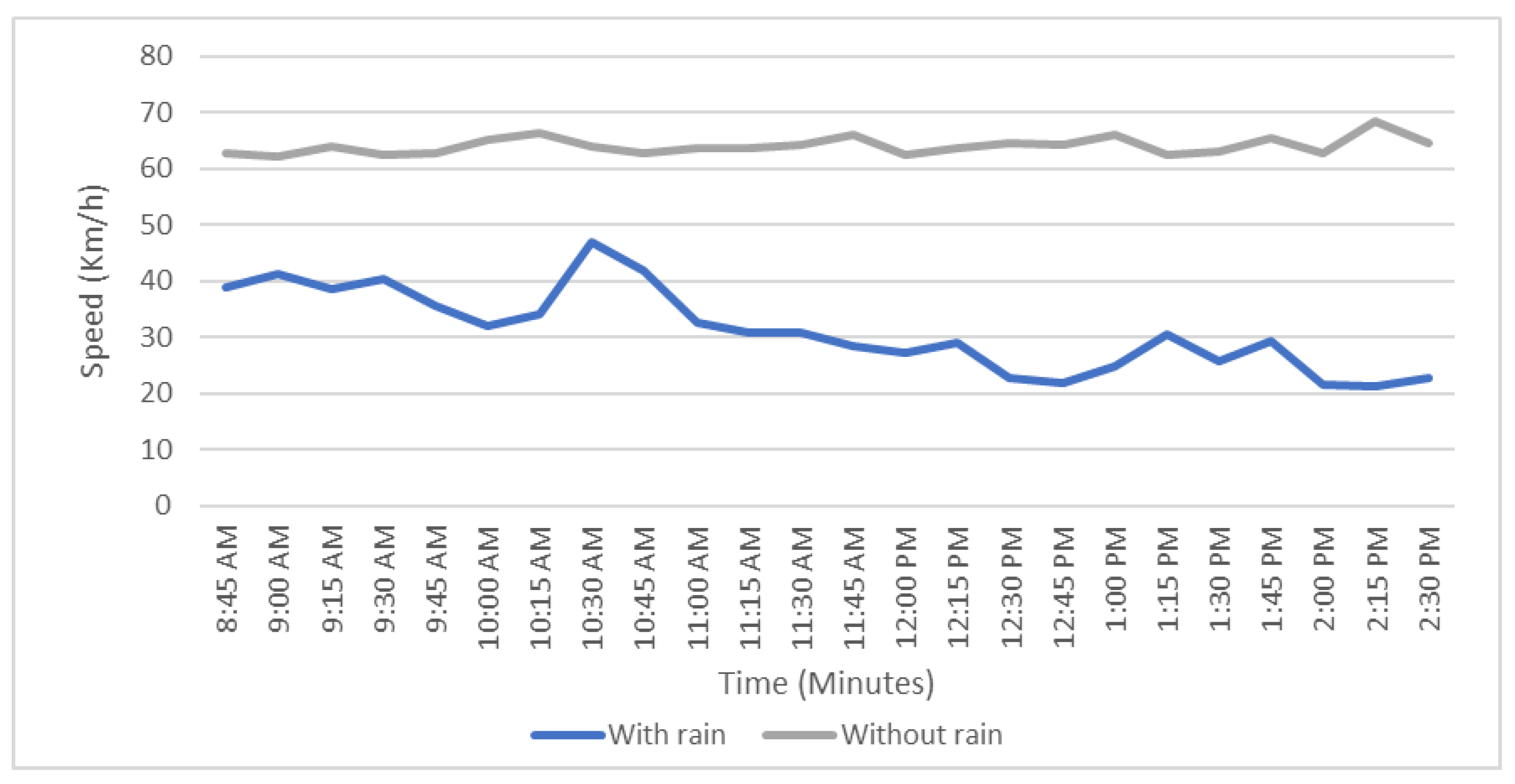
The weather data were aggregated into 15-min intervals to match the speed and flow input field observations. Figure 3 and Figure 4 show speed and flow data under rainfall conditions. The data were incorporated alongside traffic flow and speed to evaluate the model’s effectiveness under weather conditions. The x-axis shows the time between the observations, while the y-axis shows the speed/volume conditions for the selected arterial road. The blue line represents the speed/volume values during rainy days, while the grey line refers to the speed/volume values during sunny weather.

4. Model Development

This study evaluated several machine learning models, including BiLSTM, LSTM, RNN, Elman, and DLBP, based on their respective capabilities in handling sequential data and forecasting traffic flow and speed.

• LSTM and BiLSTM were chosen due to their strong ability to capture temporal dependencies and non-linear relationships in traffic data. While LSTM can model long-range dependencies in time-series data, BiLSTM enhances this by learning from past and future time steps, which is particularly beneficial for capturing the bidirectional nature of traffic patterns.
• RNN was used as a baseline model, offering a simple yet effective architecture for time-series forecasting. It was included to benchmark the performance of more complex models like LSTM and BiLSTM.
• Elman networks, a type of simple recurrent neural network, were also evaluated to investigate the performance of less complex models in traffic prediction, providing a reference for comparison with the more advanced models.
• DLBP was included to explore the potential of deep learning-based approaches in handling traffic flow prediction complexities and assess the added value of deeper architectures in this context.

Different time horizons were employed (i.e., 15 min, 30 min, 45 min and 60 min) to evaluate the models’ performance under both short-term forecasting conditions; the short-term forecasts aimed to capture rapid changes in traffic patterns.

As discussed, while deep learning models like LSTM and BiLSTM provide significant advantages for capturing complex, non-linear relationships in traffic data, they are often considered “black box” models due to their lack of transparency in showing how specific input variables affect outputs [66,67]. Although these are often seen as “black box” methods, the mathematical framework governing these models is well-defined. The following set of equations outlines how the model generates predictions. These equations govern the information flow through the network, which determines the model’s ability to predict traffic flow, speed, and volume effectively. By incorporating these equations, the interpretability of the model can be addressed, and the underlying mechanism driving the predictions can be clarified.

Long Short-Term Memory (LSTM) and Bidirectional Long-Short Term Memory (BiLSTM)

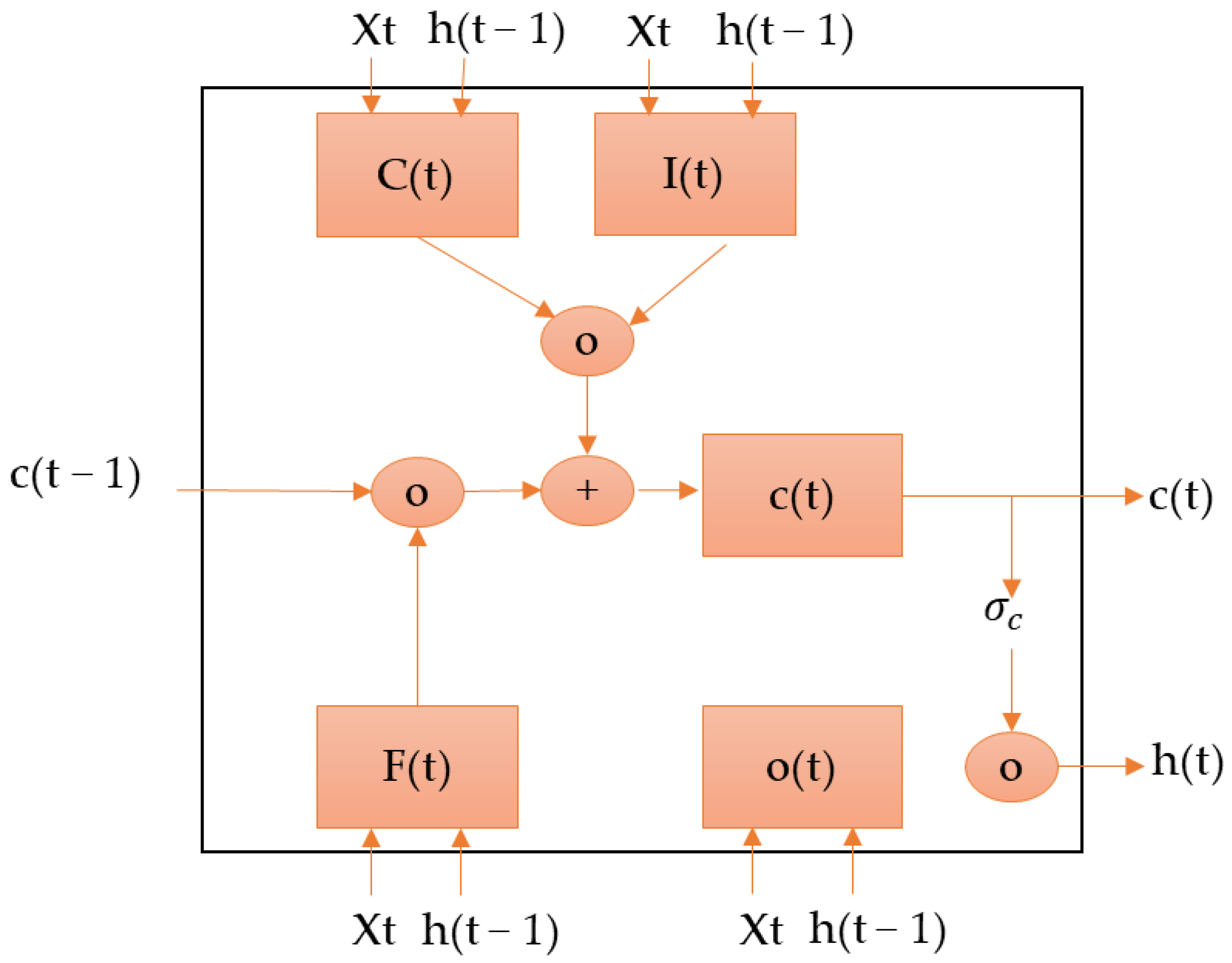
Long Short-Term Memory (LSTM) is a type of RNN model that was developed to overcome some shortcomings of conventional RNN. Because RNNs are trained using a back-propagation algorithm, the weights are impacted in the model, leading to difficulty in predicting a longer-term relationship. Long Short-Term Memory (LSTM) overcomes this issue because it has multiple gates (input gate, output gate, and forget gate), ensuring that the hidden layer’s stored values are helpful in the prediction process and pass through the output layer (Figure 5). Hence, LSTM can learn longer-term dependencies and generate better results than the RNN model.

In these models, the following formulae are used to calculate the predicted values (Matlab 2021b):

$$\mathrm{Input}\mathrm{gate}\left({\mathrm{I}}_{\mathrm{t}}\right)={\mathsf{\sigma }}_{\mathrm{g}}\left({\mathrm{W}}_{\mathrm{i}}{\mathrm{X}}_{\mathrm{t}}+{\mathrm{R}}_{\mathrm{i}}{\mathrm{h}}_{\mathrm{t}-1}+{\mathrm{b}}_{\mathrm{i}}\right)$$

(1)

$$\mathrm{Forget}\mathrm{gate}\left({\mathrm{f}}_{\mathrm{t}}\right)={\mathsf{\sigma }}_{\mathrm{g}}\left({\mathrm{W}}_{\mathrm{f}}{\mathrm{X}}_{\mathrm{t}}+{\mathrm{R}}_{\mathrm{f}}{\mathrm{h}}_{\mathrm{t}-1}+{\mathrm{b}}_{\mathrm{f}}\right)$$

(2)

$$\mathrm{Cell}\mathrm{state}\left({\mathrm{C}}_{\mathrm{t}}\right)={\mathsf{\sigma }}_{\mathrm{c}}({\mathrm{W}}_{\mathrm{c}}{\mathrm{X}}_{\mathrm{t}}+{\mathrm{R}}_{\mathrm{c}}{\mathrm{h}}_{\mathrm{t}-1}+{\mathrm{b}}_{\mathrm{c}})$$

(3)

$$\mathrm{Output}\mathrm{gate}\left({\mathrm{o}}_{\mathrm{t}}\right)={\mathsf{\sigma }}_{\mathrm{g}}\left({\mathrm{W}}_{\mathrm{o}}{\mathrm{X}}_{\mathrm{t}}+{\mathrm{R}}_{\mathrm{o}}{\mathrm{h}}_{\mathrm{t}-1}+{\mathrm{b}}_{\mathrm{o}}\right)$$

(4)

where σ_g is the gate activation function, ${\mathrm{W}}_{\mathrm{i}},{\mathrm{W}}_{\mathrm{f}},{\mathrm{W}}_{\mathrm{c}}\mathrm{a}\mathrm{n}\mathrm{d}{\mathrm{W}}_{\mathrm{o}}$ are input weight matrices, ${\mathrm{R}}_{\mathrm{i}},{\mathrm{R}}_{\mathrm{f}},{\mathrm{R}}_{\mathrm{c}}\mathrm{a}\mathrm{n}\mathrm{d}{\mathrm{R}}_{\mathrm{o}}$ are recurrent weight matrices, ${\mathrm{X}}_{\mathrm{t}}$ represents the input, ${\mathrm{h}}_{\mathrm{t}-1}$ represents the output at the previous time (t−1), and ${\mathrm{b}}_{\mathrm{i}},{\mathrm{b}}_{\mathrm{f}},{\mathrm{b}}_{\mathrm{c}}\mathrm{a}\mathrm{n}\mathrm{d}{\mathrm{b}}_{\mathrm{o}}$ are bias vectors. The “input gate” specifies new input to the cell state; the “forget gate” determines how much of the prior memory values should be removed from the “cell state”. The “cell state” and “output gate” of the LSTM at time t are calculated as follows:

Ct = ft⊙ct − 1 + it⊙gt

(5)

Ht = ot⊙σc(ct)

(6)

where ⊙ denotes the Hadamard product (element-wise multiplication of vectors).

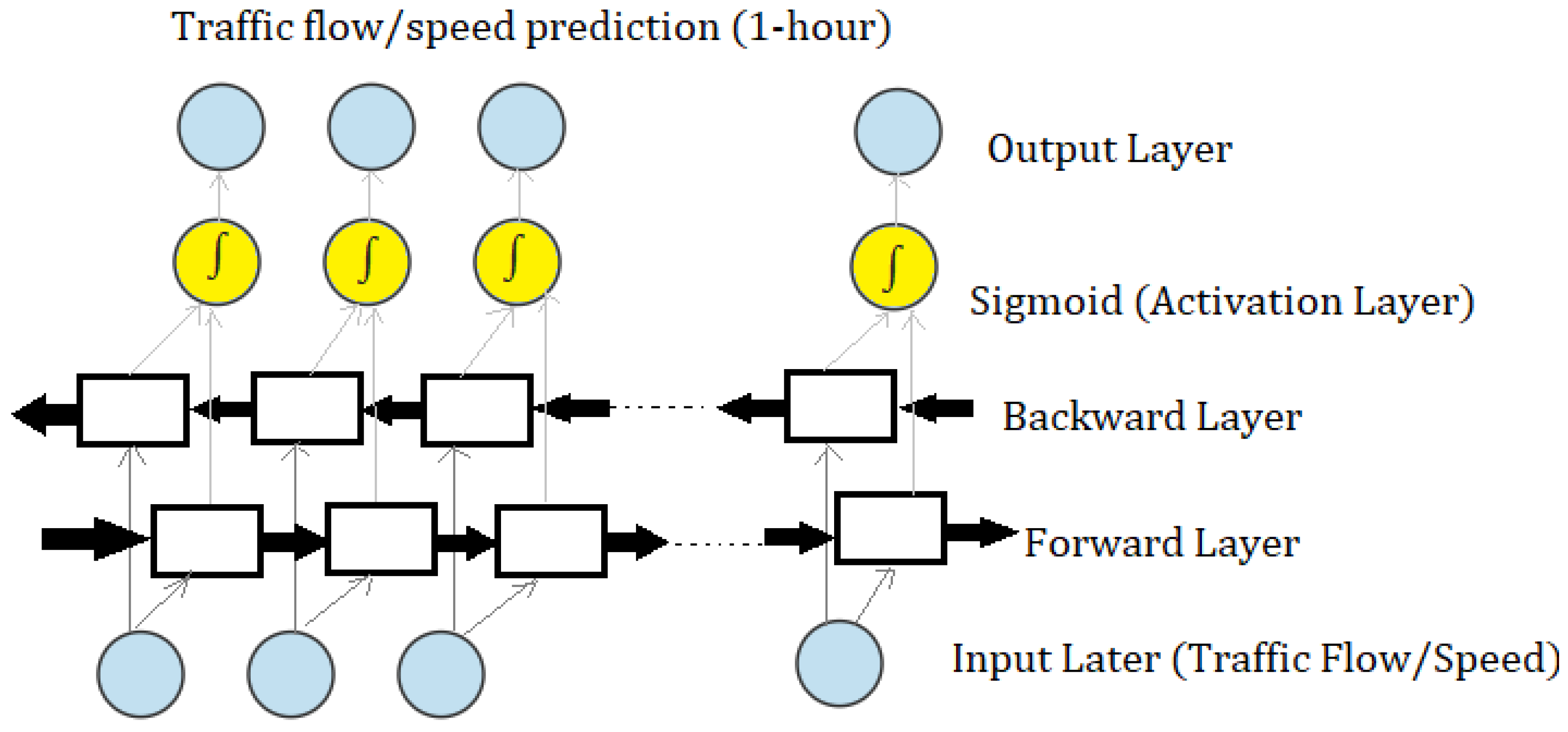
Bidirectional Long-Short Term Memory (BiLSTM) is a deep learning model that has the capability to process the input data in two directions (forward and backward), i.e., the model stores the future and the past values in comparison to LSTM (Figure 6). This helps to gain a deeper knowledge of the relationships in the sequential information fed to the network. This bidirectional processing is particularly beneficial in traffic prediction, where future states (e.g., upcoming intersections or traffic signals) can influence current traffic conditions. For example, Melbourne’s Hoddle Street’s traffic flow can be impacted by prior and upcoming signal phases and intersections. The BiLSTM’s ability to process bidirectionally allows it to leverage these dependencies, enhancing prediction accuracy in dynamic traffic environments.

When selecting a traffic prediction model, there is often a trade-off between accuracy and computational complexity. While models such as BiLSTM provide high accuracy due to their ability to capture bidirectional dependencies in data, they require more computational resources and may present challenges for real-time processing, especially when handling large datasets or when quick decision-making is essential. For real-time applications, simpler models may be preferred for faster processing times, though they may have limitations in predictive accuracy. Future studies may focus on optimising BiLSTM and other complex models to balance accuracy with computational efficiency, enabling broader applications in real-time traffic management systems.

5. Model Evaluation

Five machine learning systems were evaluated using the datasets described above. These included BiLSTM, Uni-LSTM, RNNs, Elman, and DLBP neural networks. These models have been widely used for traffic forecasts, and they were implemented using MATLAB R2020b and Neuralware Professional [68].

This study collected traffic data across all lanes of Hoddle Street during weekdays and weekends and under varying traffic conditions. The data were categorised based on time of day (e.g., peak hours, off-peak hours) and specific traffic conditions (e.g., free-flowing, congested), allowing the model to account for different patterns in traffic behaviour. Lane-specific data were also integrated, capturing variations in traffic flow across different lanes of the arterial road.

For clarity, the following variables were included in the model:

• Traffic Flow: Measured as the number of vehicles passing a specific point per unit of time.
• Traffic Speed: The average speed of vehicles at each measurement point.
• Time of Day: Categorised as peak or off-peak hours.

These variables were carefully defined and included as input features to ensure that the model could adapt to the dynamic nature of traffic on the arterial road.

In this study, the primary variables for predictions are traffic speed and volume, the dependent variables in the LSTM and BiLSTM models. It is acknowledged that the spatial location of the measurement points along the arterial road is an important factor influencing these variables; in this case, they were fixed at signalised intersections.

First, the data were arranged as two-column values. The first column corresponds to speed/volume at time t, and the second column corresponds to the expected output (t + n), where n ranges from 15 min to 60 min into the future. Then, the data were partitioned into training and testing sets. The models were trained on the first 60% of the sequence and tested on the last 40%. To prevent model overfitting, the training/testing data were standardised to have zero mean and unit variance. The DLPB model parameters used for this experiment included three hidden layers with 4, 6, and 2 neurons. The transfer function was Tanh with a learning coefficient output (α = 0.15). The learning rule was Ext DBD with 100,000 iterations and a momentum of 0.4. RNN and Elman’s models were created using one hidden layer with ten neurons, activation function (tanh), learn rule (ext DBD), and [1:2] layers delay. The BiLSTM and Uni-LSTM networks were created using four layers: sequence input layer (number of features = 1), Uni-LSTM/BiLSTM layers (number of hidden units = 300), fully connected layer (number of responses = 1), and regression layer. The model hyperparameter settings are presented in

Table 2. Model hyperparameters for Uni-LSTM and BiLSTM.

Parameters	Values
Gradient decay factor	0.9
Initial learning rate	0.005
Minimum batch size	128
Maximum epochs	300
Training optimiser	Adaptive moment estimation optimiser
Dropping learning rate during training	Piecewise
Learning rate drop period	125
The factor for the learning rate dropping	0.2

. The experiments were also implemented with the Deep Learning Toolbox functions of trainNetwork, training options, and predictAndUpdateState using the following hyperparameters [69,70].

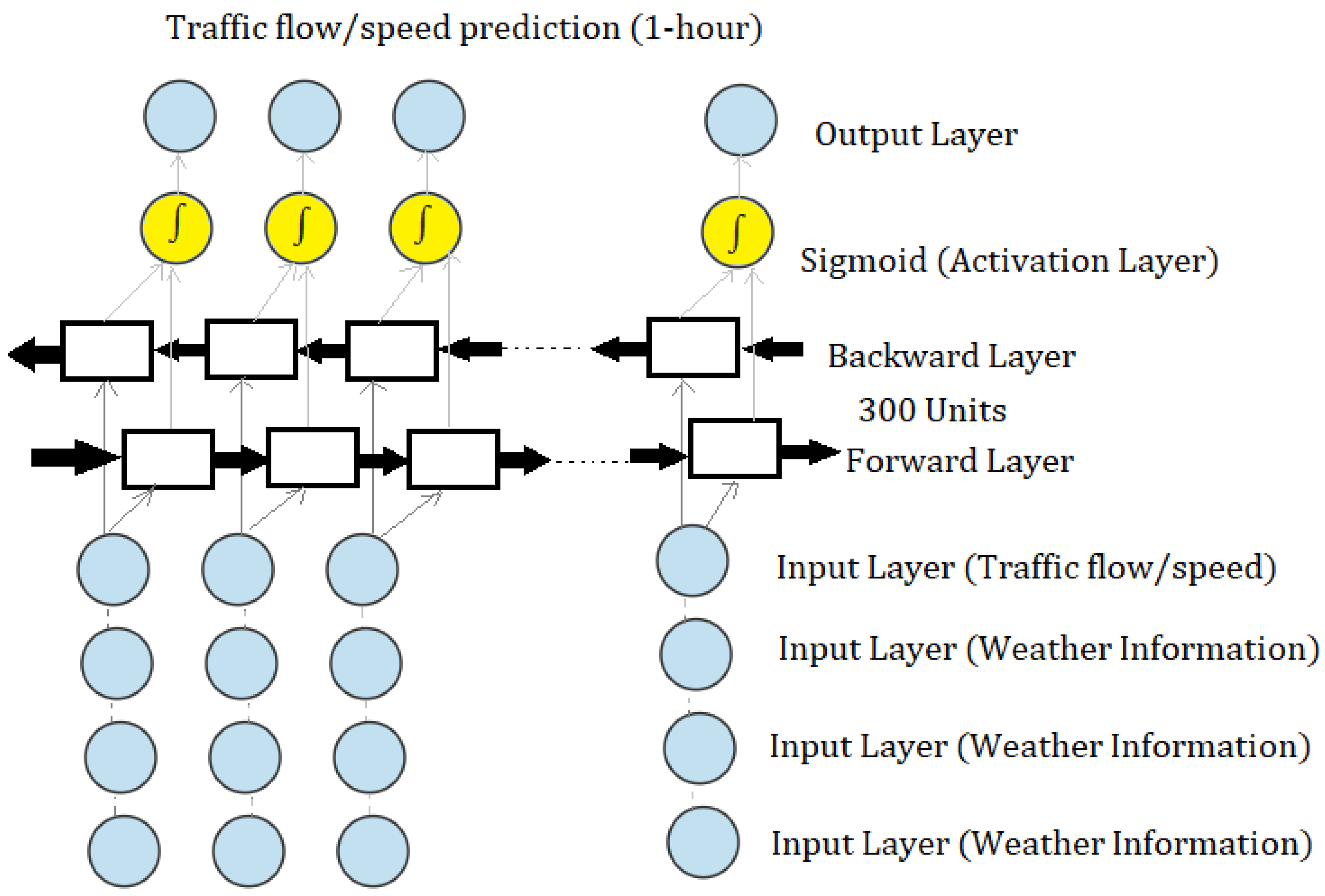
A total of four experiments were tested with the model. The first two experiments predicted speed and flow traffic conditions for up to 1 h using only flow and speed information as inputs (Figure 7). The other two experiments explored the impacts of multiple weather data on traffic flow and speed prediction for up to 1 h into the future (Figure 8). See the figures below for architecture and model representation.

5.1. Model Experiment 1: Speed Prediction

The data for speed and traffic volumes were divided into 60% training data and 40% testing data. The mean absolute percentage error (MAPE) was used to calculate the accuracy of the model prediction for different time horizons. MAPE measurements were used to calculate the average absolute difference between the predicted output from the model (Y1) and the expected true output (Y):

$$\mathrm{MAPE}(\%)=({\displaystyle \frac{1}{n}}{\sum }_{i=1}^n{\displaystyle \frac{|Y-Y_1|}{Y}})\times 100$$

(7)

Accuracy (%) = (100 − MAPE)

(8)

The speed results from the northbound direction (

Table 3. Speed prediction accuracy results for northbound and southbound directions.

Prediction Horizons	Speed (km/h) Northbound
	BiLSTM		Uni-LSTM		RNN		Elman		DLBP
	MAPE (%)	Accuracy (%)	MAPE (%)	Accuracy (%)	MAPE (%)	Accuracy (%)	MAPE (%)	Accuracy (%)	MAPE (%)	Accuracy (%)
15 min	0.07%	99.93%	8.63%	91.37%	10.77%	89.23%	10.88%	89.12%	11.16%	88.84%
30 min	0.14%	99.86%	9.24%	90.76%	12.74%	87.26%	12.72%	87.28%	12.85%	87.15%
45 min	0.11%	99.89%	9.21%	90.79%	12.78%	87.22%	12.67%	87.33%	16.17%	83.83%
60 min	0.16%	99.84%	9.42%	90.58%	13.74%	86.26%	13.62%	86.38%	12.89%	87.11%
Prediction Horizons	Speed (km/h) Southbound
	BiLSTM		LSTM		RNN		Elman		DLBP
	MAPE (%)	Accuracy (%)	MAPE (%)	Accuracy (%)	MAPE (%)	Accuracy (%)	MAPE (%)	Accuracy (%)	MAPE (%)	Accuracy (%)
15 min	0.13%	99.87%	11.24%	88.76%	13.94%	86.06%	14.06%	85.94%	16.06%	83.94%
30 min	0.14%	99.86%	12.35%	87.65%	17.05%	82.95%	17.33%	82.67%	17.86%	82.14%
45 min	0.16%	99.84%	12.46%	87.54%	17.67%	82.33%	18.07%	81.93%	18.37%	81.63%
60 min	0.20%	99.80%	12.59%	87.41%	18.41%	81.59%	18.77%	81.23%	17.11%	82.89%

Note: The green cells represent the best-performing models, while the yellow cells represent the worst-performing models.

) show that BiLSTM provided the least MAPE (%) error and the best accuracy of 99% from the 15-min to the 60-min prediction horizon. The second-best model was Uni-LSTM, with an accuracy above 90% for up to a 60-min prediction horizon. For both LSTM models, the accuracy did not deteriorate substantially as the prediction horizon increased, showing the ability of the system to capture the complexity of longer speed prediction horizons. On the other hand, the RNN and Elman models provided an accuracy above 85% for up to 60-min prediction horizons, and they provided better accuracy than the DLBP model for up to 45-min prediction horizons. DLBP provided a better prediction accuracy for a longer speed prediction horizon of 60 min into the future, with an accuracy of 87%. However, the DLBP model had the lowest performance of less than 85% from 15-min to 45-min prediction horizons.

A similar result can be noticed for speeds from the southbound direction (Table 3). The green cells represent the best-performing models, while the yellow cells represent the worst-performing models. It shows that BiLSTM provided the least MAPE (%) error and the best accuracy of 99% from a 15-min to a 60-min prediction horizon. As above, the second-best model was Uni-LSTM, with an accuracy above 87% for up to a 60-min prediction horizon. On the other hand, the RNN and Elman models provided an accuracy above 81% for up to 60-min prediction horizons, and they provided better accuracy than the DLBP model for up to 45-min prediction horizons. At the same time, DLBP provided a better prediction accuracy for a longer speed prediction horizon of 60 min into the future with an accuracy of 83%. However, the DLBP model had the lowest performance among all models from 15-min to 45-min prediction horizons.

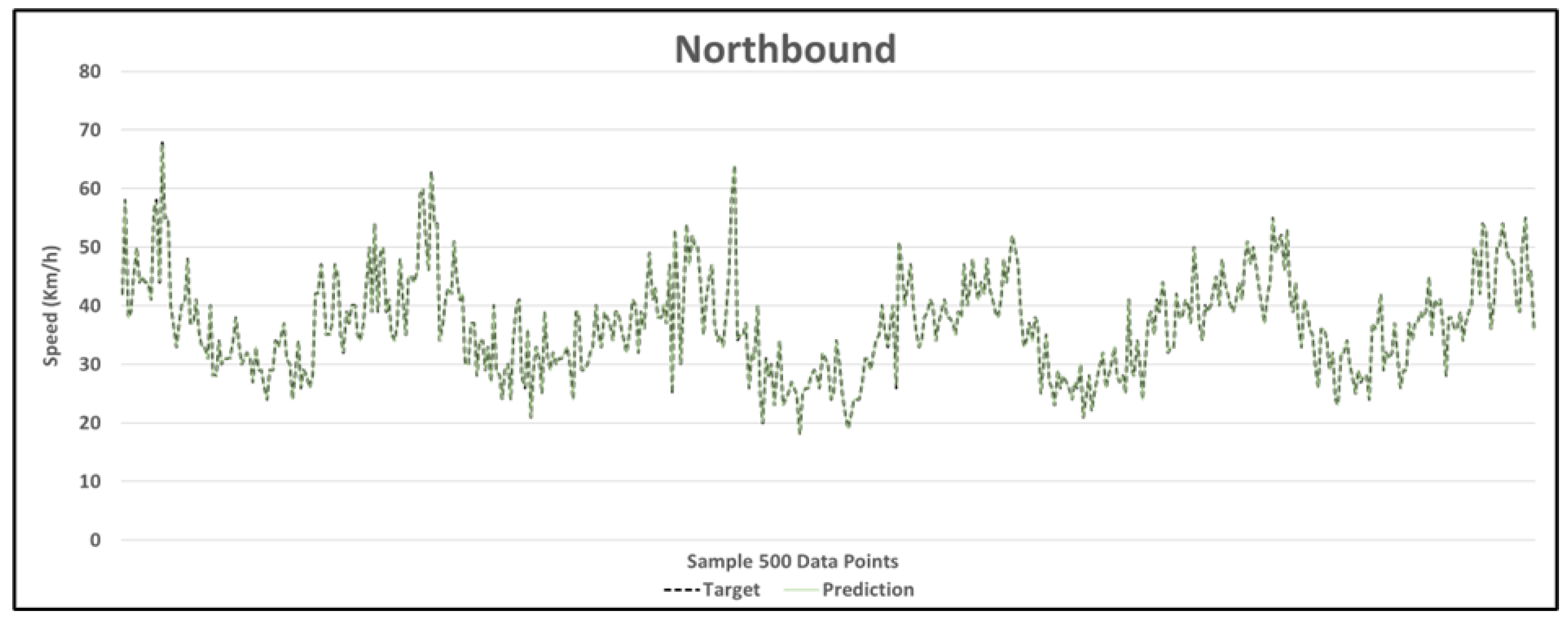
The best speed prediction performance from the BiLSTM model is illustrated in Figure 9, Figure 10, Figure 11 and Figure 12. The black dashed line represents the target real-speed data compared to the green trendline, which represents the results generated from the model.

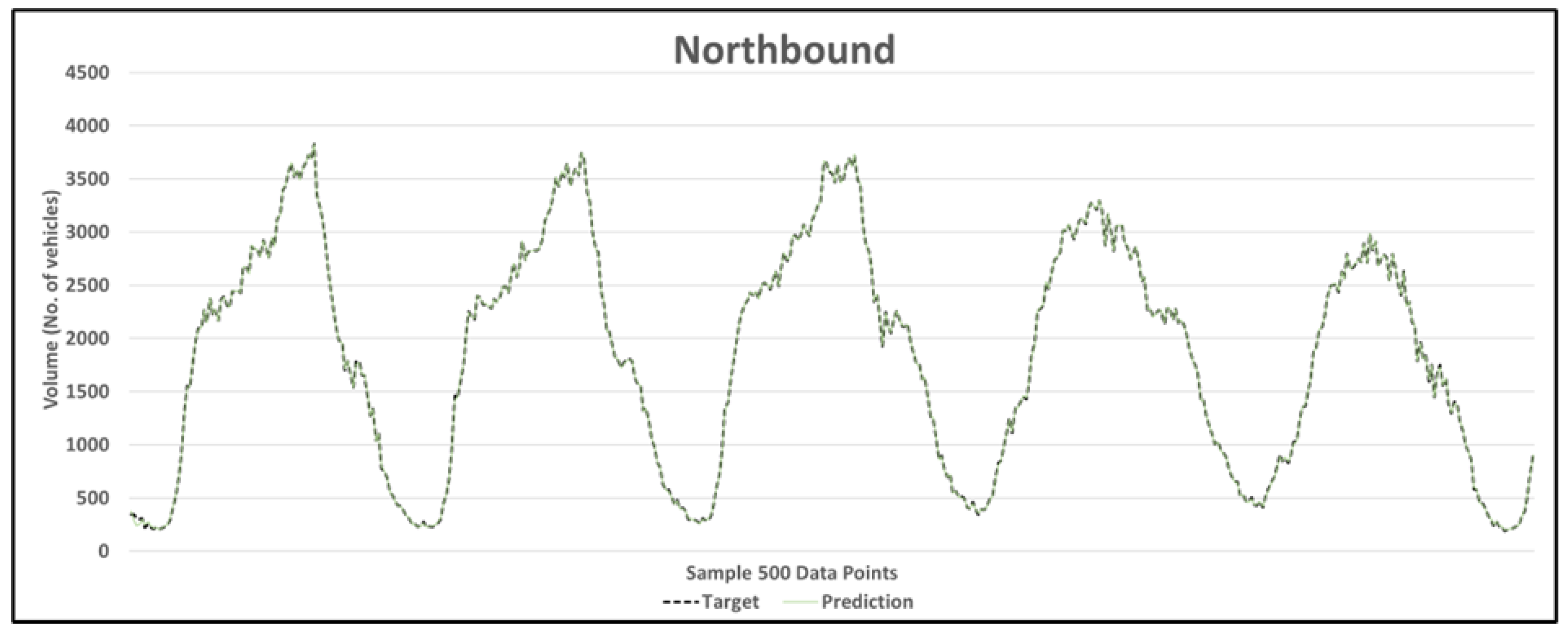
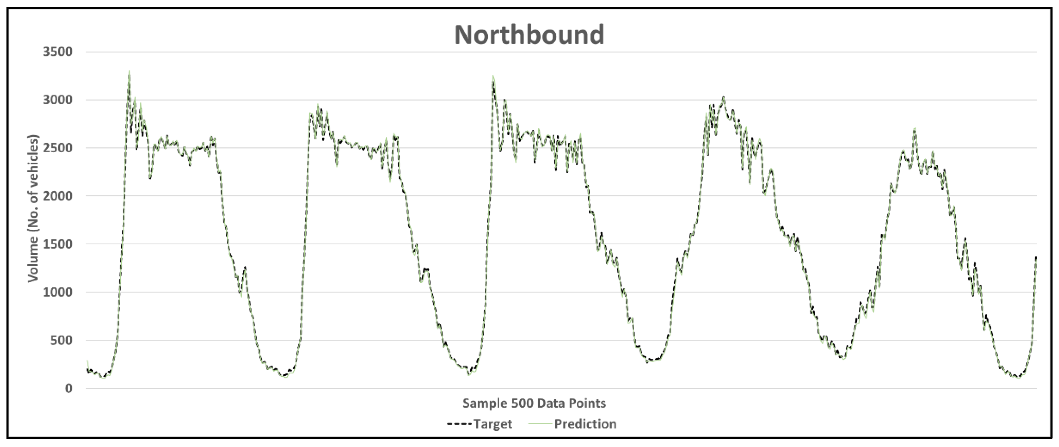
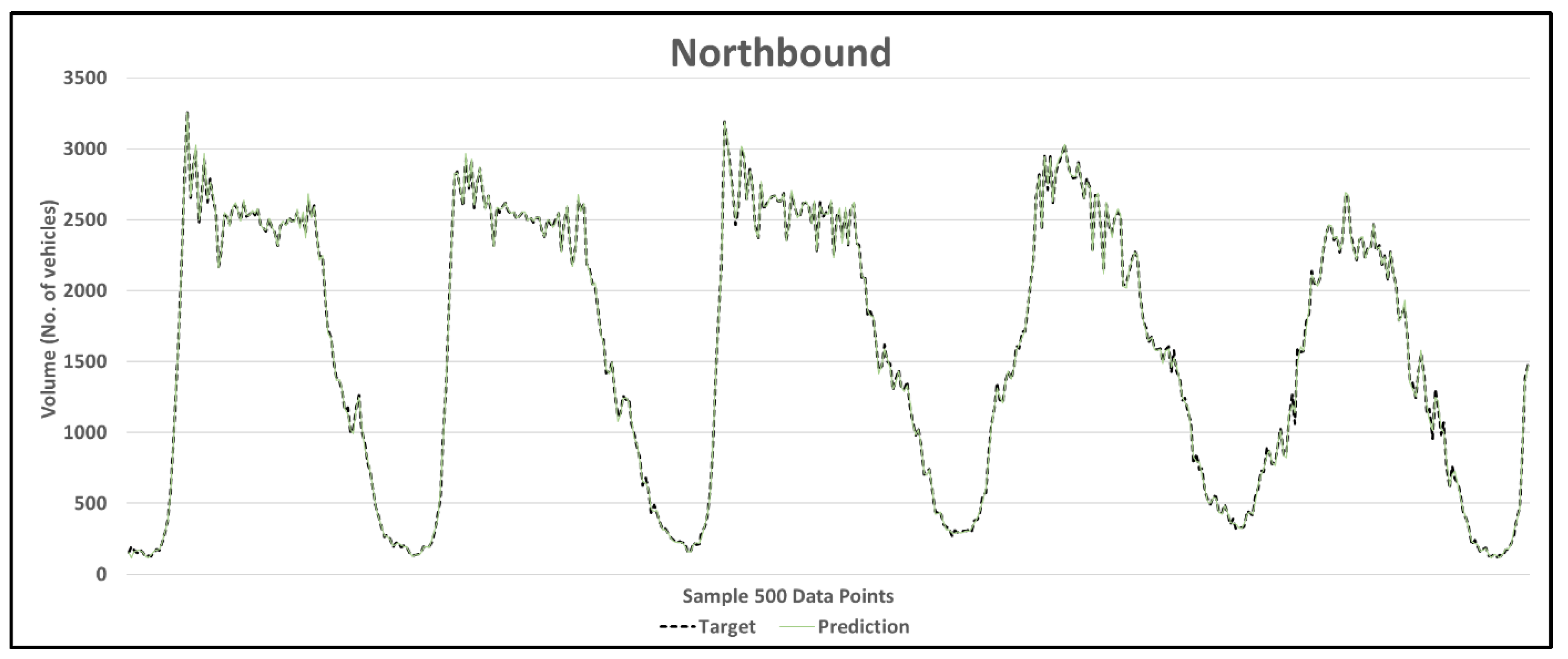
In the figures below, the x-axis represents the time period of data collection (in minutes), while the y-axis shows the speed and volume of observations. The figures compare the target values (black dashed line) with the prediction values from the developed model (green lines).

5.2. Model Experiment 2: Flow Prediction

The traffic volume results from the northbound direction (

Table 4. Volume prediction accuracies results for northbound and southbound directions.

Prediction Horizons	Volume (No. of Vehicles) Northbound
	BiLSTM		Uni-LSTM		RNN		Elman		DLBP
	MAPE (%)	Accuracy (%)	MAPE (%)	Accuracy (%)	MAPE (%)	Accuracy (%)	MAPE (%)	Accuracy (%)	MAPE (%)	Accuracy (%)
15 min	0.54%	99.46%	4.77%	95.23%	7.32%	92.68%	7.30%	92.70%	8.38%	91.62%
30 min	2.37%	97.63%	5.12%	94.88%	12.41%	87.59%	12.34%	87.66%	11.68%	88.32%
45 min	3.20%	96.80%	5.13%	94.87%	18.17%	81.83%	17.86%	82.14%	17.58%	82.42%
60 min	3.18%	96.82%	5.92%	94.08%	24.46%	75.54%	24.03%	75.97%	21.45%	78.55%
Prediction Horizons	Volume (No. of Vehicles) Southbound
	BiLSTM		LSTM		RNN		Elman		DLBP
	MAPE (%)	Accuracy (%)	MAPE (%)	Accuracy (%)	MAPE (%)	Accuracy (%)	MAPE (%)	Accuracy (%)	MAPE (%)	Accuracy (%)
15 min	1.07%	98.93%	6.80%	93.20%	9.43%	90.57%	9.38%	90.62%	9.86%	90.14%
30 min	1.24%	98.76%	7.67%	92.33%	15.23%	84.77%	14.90%	85.10%	13.94%	86.06%
45 min	2.15%	97.85%	8.67%	91.33%	22.18%	77.82%	21.32%	78.68%	23.58%	76.42%
60 min	3.87%	96.13%	9.87%	90.13%	28.67%	71.33%	29.05%	70.95%	26.96%	73.04%

Note: The green cells represent the best-performing models, while the yellow cells represent the worst-performing models.

) show that BiLSTM provided the least MAPE (%) error and the best accuracy, ranging from 99% to 96% from the 15-min to 60-min prediction horizon. The second-best model was Uni-LSTM, with an accuracy above 94% for up to a 60-min prediction horizon. On the other hand, the RNN and Elman models provided an accuracy above 82% for up to 45-min prediction; then, it decreased to 75% for 60-min prediction horizons. DLBP provided a better prediction accuracy compared to RNN and Elman for a longer speed prediction horizon of 60 min into the future, with an accuracy of 78%.

The traffic volume results from the southbound direction (Table 4) show that BiLSTM provided the least MAPE (%) error and the best accuracy, ranging from 99% to 96% from a 15-min to a 60-min prediction horizon. The green cells represent the best-performing models, while the yellow cells represent the worst-performing models. The second-best model was Uni-LSTM, with an accuracy above 93% for up to a 60-min prediction horizon. On the other hand, the RNN and Elman models provided an accuracy above 78% for up to 45-min prediction; then, it decreased to 71% for 60-min prediction horizons. DLBP provided a better prediction accuracy compared to RNN and Elman for a longer speed prediction horizon of 60 min into the future, with an accuracy of 73%.

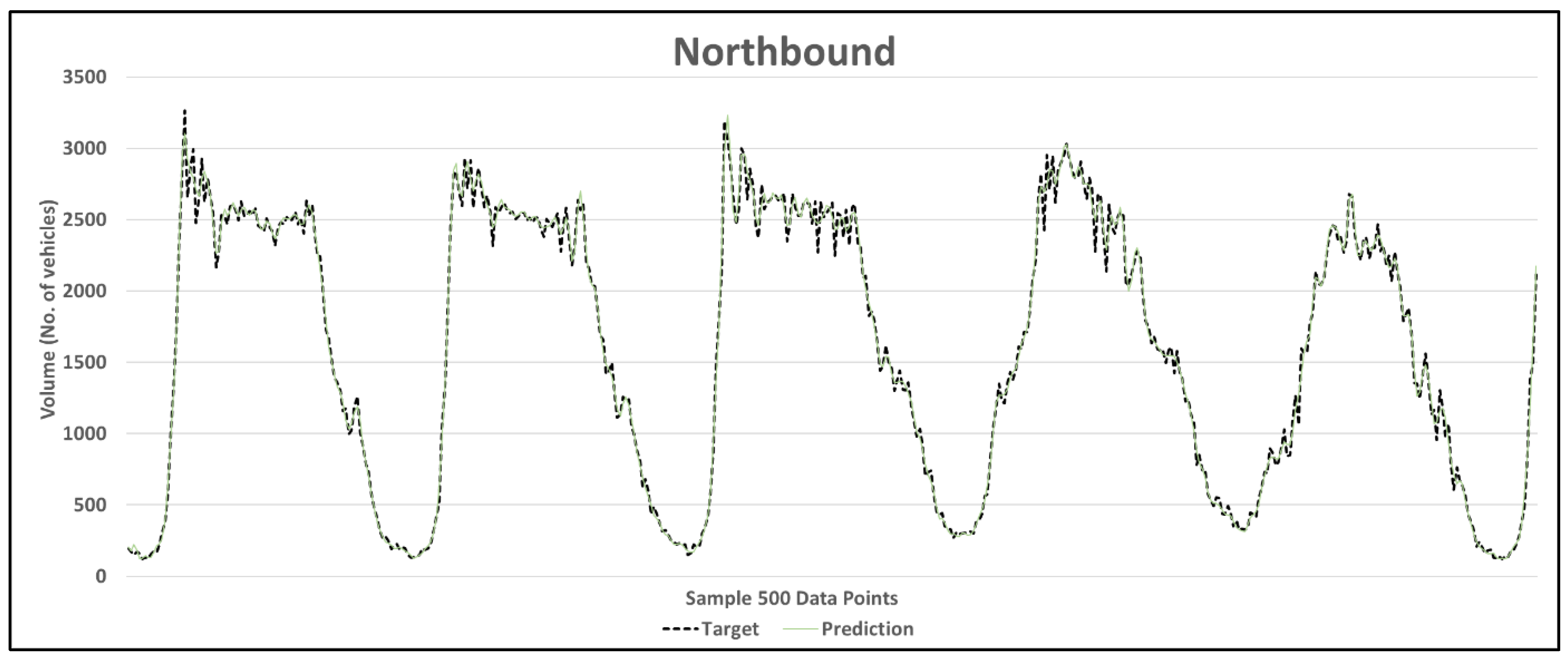
The best traffic volume prediction performance from the BiLSTM model is illustrated in Figure 13, Figure 14, Figure 15 and Figure 16. The black dashed line represents the target real volume data compared to the green trendline, which represents the results generated from the model. In the figures below, the x-axis represents the time period of data collection (in minutes), while the y-axis shows the speed and volume of observations. The figures compare the target values (black dashed line) with the prediction values from the developed model (green lines).

5.3. Model Experiment 3: Weather Integrated Speed Prediction

The weather conditions incorporated in this experiment included rainfall observation in mm, air temperature in degrees Celsius, relative humidity in percentage % and wind speed in km/h. Weather data were gathered at 1-min intervals, and speed data were gathered every 15 min; the weather data were then aggregated into 15-min intervals to match the frequency of the traffic data. These models achieved the highest performance in the previous experiments when tested in the northbound and southbound directions. Hence, multiple BiLSTM and LSTM scenarios were trained/tested under different weather conditions to evaluate the model’s robustness. The total observations used in all scenarios were 35,036 observations for speed and weather information, with 21,022 observations used for training and 14,014 observations used for testing/validation.

In the first scenario, “BiLSTM_No weather”, the input only included the average speed (northbound and southbound directions). The results for this scenario demonstrated a high accuracy for the BiLSTM model above 99% for multiple prediction horizons. For the “LSTM_No weather” scenario, the results also showed a high level of accuracy above 91% for multiple prediction horizons up to 60 min into the future. For the second scenario, “BiLSTM_Rain” and “LSTM_Rain”, the input data included two features: speed (km/h) and rain intensity (mm). The results for the BiLSTM model showed a similar accuracy of above 99% for multiple prediction horizons and above 91% for the LSTM model for up to 60 min into the future (

Table 5. Speed prediction accuracies under multiple weather conditions results.

Prediction Horizons	Speed (km/h)
	15 min		30 min		45 min		60 min
	MAPE (%)	Accuracy (%)	MAPE (%)	Accuracy (%)	MAPE (%)	Accuracy (%)	MAPE (%)	Accuracy (%)
BiLSTM_No weather	0.12	99.88	0.15	99.85	0.17	99.83	0.25	99.75
BiLSTM_Rain	0.40	99.60	0.28	99.72	0.41	99.59	2.02	97.98
BiLSTM_Rain and Wind	0.30	99.70	0.23	99.77	0.55	99.45	1.91	98.09
BiLSTM_Weather	0.21	99.79	0.32	99.68	0.32	99.68	0.23	99.77
LSTM_No weather	7.08	92.92	7.76	92.24	7.87	92.13	8.09	91.91
LSTM_Rain	7.40	92.60	8.07	91.93	8.32	91.68	8.47	91.53
LSTM_Rain and Wind	7.40	92.60	8.18	91.82	8.22	91.78	8.38	91.62
LSTM_All Weather	7.34	92.66	8.04	91.96	8.18	91.82	8.35	91.65

). The third scenario, “BiLSTM_Rain and Wind” and “LSTM_Rain and Wind”, incorporated three inputs: speed data with rain and wind speed. The results showed prediction accuracies above 99% and 91% for BiLSTM and LSTM, respectively. The last scenario, “BiLSTM_Weather” and “LSTM_Weather”, involved five inputs: speed, rain, wind speed and humidity and air temperature. The results for both models demonstrate the robustness of the models when tested under multiple weather conditions with an accuracy above 99% for the BiLSTM model and 91% for the LSTM model. The green cells in Table 5 represent the best-performing models, while the yellow cells represent the worst-performing models.

5.4. Model Experiment 4: Weather Integrated Volume Prediction

The results for this scenario demonstrated a high accuracy for the BiLSTM model above 96% for multiple prediction horizons. For the “LSTM_No weather” scenario, the results also showed a high level of accuracy above 93% for multiple prediction horizons up to 60 min into the future. In the second scenario, “BiLSTM_Rain” and “LSTM_Rain”, the input data included two features: traffic volume and rain data. The results for the BiLSTM model maintained a similar accuracy above 96% for multiple prediction horizons and above 93% for the LSTM model for up to 60 min into the future. The third scenario, “BiLSTM_Rain and Wind” and “LSTM_Rain and Wind”, incorporated three inputs: volume data with rain and wind speed. The results showed prediction accuracies above 96% and 93% for BiLSTM and LSTM, respectively. The last scenario, “BiLSTM_Weather” and “LSTM_Weather”, involved five inputs: volume, rain, wind speed and humidity and air temperature. The results for both models demonstrated the robustness of the models when tested under multiple weather conditions with an accuracy above 96% for the BiLSTM model and 93% for the LSTM model (

Table 6. Volume prediction accuracies under multiple weather conditions results.

Prediction Horizons	Volume (No. of Vehicles)
	15 min		30 min		45 min		60 min
	MAPE (%)	Accuracy (%)	MAPE (%)	Accuracy (%)	MAPE (%)	Accuracy (%)	MAPE (%)	Accuracy (%)
BiLSTM_No weather	1.16	98.84	2.46	97.54	2.38	97.62	3.14	96.86
BiLSTM_Rain	0.87	99.13	2.47	97.53	2.62	97.38	2.87	97.13
BiLSTM_Rain and Wind	2.34	97.66	2.60	97.40	2.75	97.25	2.87	97.13
BiLSTM_Weather	2.13	97.87	2.40	97.60	3.42	96.58	2.94	97.06
LSTM_No weather	4.37	95.63	4.60	95.40	4.89	95.11	5.97	94.03
LSTM_Rain	5.02	94.98	5.03	94.97	5.39	94.61	6.00	94.00
LSTM_Rain and Wind	4.73	95.27	5.52	94.48	5.37	94.63	6.19	93.81
LSTM_All Weather	4.93	95.07	5.50	94.50	5.86	94.14	6.61	93.39

). It can also be noticed that incorporating weather data into BiLSTM led to a minor improvement in the accuracy for multiple prediction horizons. For example, the prediction increased the most when traffic volume was trained and tested with rainfall intensities for 15-min prediction horizons. For 60-min prediction horizons, volume with rain and wind improved the accuracy to 97.13% when compared to 96.86% without weather information. However, the overall results demonstrated the robustness of the model in achieving high prediction accuracy when trained/tested under variable weather conditions. The green cells represent the best-performing models, while the yellow cells represent the worst-performing models.

6. Analysis of Results

The BiLSTM models were shown to outperform other prediction models such as ELMAN, RNN and LSTM. The accuracy improvement percentages ranged between 2% and 6% for traffic volume prediction in both travel directions for up to 60 min into the future. The accuracy ranged between 96% and 99% for multiple prediction horizons for both directions. A greater improvement can be noticed for speed prediction, ranging between 9% and 12% for both travel directions. The accuracy ranged between 99.80% and 99.93% for up to 60 min into the future.

This study also focused on the impact of weather on traffic prediction performance. When rain intensities (in mm) are added to the inputs, the flow performance is not affected for a prediction horizon of up to 30 min. However, a slight improvement can be noticed for the 60-min prediction horizon through an increase from an accuracy of 96.86% to 97.13%. On the other hand, no improvement was noticed for speed predictions, noting that the previous accuracy was above 99% and it is hard to outperform that by adding more features, such as weather information. Another experiment included adding both rain and wind speed to the traffic flow and speed inputs. However, no improvement could be observed in model performance for both speed and flow for multiple prediction horizons.

The last experiment included adding multiple types of weather information (rain intensity, wind speed, humidity and air temperature) to the traffic information inputs. The results showed a minimal improvement in traffic flow prediction from 97.54% to 97.60% for the 30-min prediction horizons and from 96.86% to 97.60% for the 60-min prediction horizons. For speed prediction, the only improvement noticed was for the 60-min prediction horizon, with a minimal enhancement from 99.75% to 99.77%. This shows that adding weather information can enhance the model only if the initial traffic information is not performing well as inputs to the model. Adding weather information data to the inputs also provided good accuracy overall, similar to the initial results, with minor enhancements to a few traffic prediction horizons for both speed and flow. However, adding weather information to the model has practical implications for the public, who might want to know how their travel is impacted by severe weather conditions on their travel routes.

In this study, the BiLSTM model demonstrated superior performance in predicting traffic flow compared to the unidirectional LSTM. A comparison with other neural network models, such as RNN, Elman, and DLBP, is provided to contextualise these findings further, as shown in Table 3, Table 4, Table 5 and Table 6. This comparative analysis allows a clearer understanding of BiLSTM’s advantages and limitations in various forecasting scenarios.

The performance disparities between the LSTM and BiLSTM models observed in this study can be attributed to their architectural differences and how each model processes temporal dependencies. The unidirectional LSTM model processes data in a forward direction, limiting its ability to capture dependencies that rely on future and past information. This can impact prediction accuracy in cases where forward-looking context is crucial, such as predicting sudden traffic changes influenced by upcoming intersections or congestion.

On the other hand, the BiLSTM model processes sequences in both forward and backward directions, enabling it to be influenced by information from past and future states. This bidirectional processing allows BiLSTM to capture complex, fluctuating traffic conditions. As a result, the BiLSTM model demonstrated higher accuracy, especially in scenarios where traffic flow is influenced by prior and forthcoming events, leading to improved predictions over the unidirectional LSTM model.

7. Conclusions

In this study, unidirectional and bidirectional LSTM models were developed using data from a busy arterial road in Melbourne, Australia, to predict speed and traffic volumes. The models were trained/tested using historical field data collected by Intelematics INSIGHT Studio for a forecasting horizon up to 60 min into the future. A total of 70,072 data observations were extracted for a 12-month period from Hoddle Street’s southbound and northbound directions. The data represented different patterns and variable traffic conditions, including peak, non-peak, weekday, weekend, and incident data.

A comprehensive and rigorous procedure was adopted to evaluate the suitability of different architectures and modelling parameters. The results showed superior performance for the BiLSTM compared to unidirectional Uni-LSTM, RNN, Elman and DLBP for both speed and traffic volume forecasts. For speed, the model was able to provide a prediction accuracy above 99% for up to 60 min into the future in both directions (southbound and northbound). For volume, the BiLSTM model was able to achieve an accuracy above 96% for up to 60 min into the future in both directions (northbound and southbound). It was also noticed that the accuracy did not deteriorate substantially as the prediction horizon increased, which shows the ability of the system to capture the complexity of longer speed/volume prediction horizons.

The study also investigated the robustness of the AI models when developed under variable weather conditions such as rainfall observation in mm, air temperature in degrees Celsius, relative humidity and wind (1 min) speed in km/h. The experimental results showed that BiLSTM and LSTM models can effectively predict traffic speed/volume under various weather conditions.

In summary, the results showed that the model has excellent stability and prediction accuracy when tested on data collected from an arterial road. The analysis also highlighted the robustness of deep learning models when incorporating weather data, with a slight improvement in prediction accuracy achieved in some instances.

Accurate traffic prediction models have significant implications for emergency response and disaster management. Models such as BiLSTM, which can accurately forecast traffic conditions even under dynamic or incomplete data conditions, are essential for planning evacuation routes, prioritising emergency vehicle access, and optimising traffic flow during crises. By anticipating congestion points and adjusting response routes based on predicted traffic volumes and speeds, authorities can improve the safety and efficiency of emergency operations, ensuring timely assistance and enhancing community resilience in disaster scenarios.

While this study demonstrates the effectiveness of BiLSTM models in traffic prediction, future research should focus on a more detailed statistical analysis of weather variables to further enhance model robustness. Methods such as correlation analysis, regression models, and sensitivity analysis can help identify weather factors—such as rain intensity, wind speed, humidity, and temperature—that significantly impact traffic flow and speed predictions. Future studies could also benefit from case studies examining model performance under varied weather conditions (e.g., heavy rain, fog, snow) to assess prediction accuracy in challenging contexts. Additionally, investigating the temporal effects of weather on traffic, as well as interactions with other factors (e.g., time of day, special events), could provide a holistic view of weather impacts. These insights would improve the applicability of BiLSTM models for Intelligent Transport Systems (ITS) under diverse environmental conditions.

References

1. Bartlett, Z.; Han, L.; Nguyen, T.T.; Johnson, P. A machine learning based approach for the prediction of road traffic flow on urbanised arterial roads. In Proceedings of the 2018 IEEE 20th International Conference on High Performance Computing and Communications; IEEE 16th International Conference on Smart City; IEEE 4th International Conference on Data Science and Systems (HPCC/SmartCity/DSS), Exeter, UK, 28–30 June 2018; IEEE: Piscataway, NJ, USA, 2018; pp. 1285–1292. [Google Scholar]
2. Mackenzie, J.; Roddick, J.F.; Zito, R. An evaluation of HTM and LSTM for short-term arterial traffic flow prediction. IEEE Trans. Intell. Transp. Syst. 2018, 20, 1847–1857. [Google Scholar] [CrossRef]
3. Cui, Z.; Ke, R.; Pu, Z.; Wang, Y. Deep bidirectional and unidirectional LSTM recurrent neural network for network-wide traffic speed prediction. arXiv 2018, arXiv:1801.02143. [Google Scholar]
4. Cui, Z.; Ke, R.; Pu, Z.; Wang, Y. Stacked bidirectional and unidirectional LSTM recurrent neural network for forecasting network-wide traffic state with missing values. Transp. Res. Part C Emerg. Technol. 2020, 118, 102674. [Google Scholar] [CrossRef]
5. Kouziokas, G.N. Deep bidirectional and unidirectional LSTM neural networks in traffic flow forecasting from environmental factors. In Advances in Mobility-as-a-Service Systems, Proceedings of 5th Conference on Sustainable Urban Mobility, Virtual CSUM2020, Volos, Greece, 17–19 June 2020; Springer: Berlin/Heidelberg, Germany, 2021; pp. 171–180. [Google Scholar]
6. Lippi, M.; Bertini, M.; Frasconi, P. Short-term traffic flow forecasting: An experimental comparison of time-series analysis and supervised learning. IEEE Trans. Intell. Transp. Syst. 2013, 14, 871–882. [Google Scholar] [CrossRef]
7. Lund, R. Time Series Analysis and Its Applications: With R Examples; Taylor & Francis: Abingdon, UK, 2007. [Google Scholar]
8. Papageorgiou, M.; Diakaki, C.; Dinopoulou, V.; Kotsialos, A.; Wang, Y. Review of road traffic control strategies. Proc. IEEE 2003, 91, 2043–2067. [Google Scholar] [CrossRef]
9. Vlahogianni, E.I.; Karlaftis, M.G.; Golias, J.C. Short-term traffic forecasting: Where we are and where we’re going. Transp. Res. Part C Emerg. Technol. 2014, 43, 3–19. [Google Scholar] [CrossRef]
10. Jiang, B.; Fei, Y. Vehicle speed prediction by two-level data driven models in vehicular networks. IEEE Trans. Intell. Transp. Syst. 2016, 18, 1793–1801. [Google Scholar] [CrossRef]
11. Song, Z.; Guo, Y.; Wu, Y.; Ma, J. Short-term traffic speed prediction under different data collection time intervals using a SARIMA-SDGM hybrid prediction model. PLoS ONE 2019, 14, e0218626. [Google Scholar] [CrossRef]
12. Yang, F.; Yin, Z.; Liu, H.; Ran, B. Online recursive algorithm for short-term traffic prediction. Transp. Res. Rec. 2004, 1879, 1–8. [Google Scholar] [CrossRef]
13. Kalman, R.E. A New Approach to Linear Filtering and Prediction Problems. J. Basic Eng. 1960, 82, 35–45. [Google Scholar] [CrossRef]
14. Lv, Y.; Duan, Y.; Kang, W.; Li, Z.; Wang, F.-Y. Traffic flow prediction with big data: A deep learning approach. IEEE Trans. Intell. Transp. Syst. 2014, 16, 865–873. [Google Scholar] [CrossRef]
15. Lee, W.H.; Tseng, S.S.; Shieh, J.L.; Chen, H.H. Discovering Traffic Bottlenecks in an Urban Network by Spatiotemporal Data Mining on Location-Based Services. IEEE Trans. Intell. Transp. Syst. 2011, 12, 1047–1056. [Google Scholar] [CrossRef]
16. Stathopoulos, A.; Karlaftis, M.G. A multivariate state space approach for urban traffic flow modeling and prediction. Transp. Res. Part C Emerg. Technol. 2003, 11, 121–135. [Google Scholar] [CrossRef]
17. Abduljabbar, R.; Dia, H. A deep learning approach for freeway vehicle speed and flow prediction. In Proceedings of the Australasian Transport Research Forum, Canberra, Australia, 30 September–2 October 2019. [Google Scholar]
18. Ding, Q.Y.; Wang, X.F.; Zhang, X.Y.; Sun, Z.Q. Forecasting traffic volume with space-time ARIMA model. Adv. Mater. Res. 2011, 156, 979–983. [Google Scholar] [CrossRef]
19. Williams, B.M.; Hoel, L.A. Modeling and forecasting vehicular traffic flow as a seasonal ARIMA process: Theoretical basis and empirical results. J. Transp. Eng. 2003, 129, 664–672. [Google Scholar] [CrossRef]
20. Karlaftis, M.G.; Vlahogianni, E.I. Statistical methods versus neural networks in transportation research: Differences, similarities and some insights. Transp. Res. Part C Emerg. Technol. 2011, 19, 387–399. [Google Scholar] [CrossRef]
21. Dia, H.; Rose, G. Development and evaluation of neural network freeway incident detection models using field data. Transp. Res. Part C Emerg. Technol. 1997, 5, 313–331. [Google Scholar] [CrossRef]
22. Thomas, K.; Dia, H. Comparative Evaluation of Freeway Incident Detection Models Using Field Data. In IEE Proceedings-Intelligent Transport Systems; IET: Stevenage, UK, 2006; Volume 153, pp. 230–241. [Google Scholar]
23. Thomas, K.; Dia, H. Neural network incident detection on arterials using fusion of simulated probe vehicle and loop detector data. In Proceedings of the 12th ITS World Congress, San Francisco, CA, USA, 6–10 November 2005; pp. 1–12. [Google Scholar]
24. Thomas, K.; Dia, H.; Cottman, N. Simulation of arterial incident detection using neural networks. In Proceedings of the 8th World Congress on Intelligent Transport Systems, Sydney, Australia, 30 September–4 October 2001. [Google Scholar]
25. CVan Hinsbergen, I.; Van Lint, J.; Van Zuylen, H. Bayesian committee of neural networks to predict travel times with confidence intervals. Transp. Res. Part C Emerg. Technol. 2009, 17, 498–509. [Google Scholar] [CrossRef]
26. Ahmed, M.S.; Cook, A.R. Analysis of Freeway Traffic Time-Series Data by Using Box-Jenkins Techniques; Transportation Research Board: Washington, DC, USA, 1979. [Google Scholar]
27. Guo, J.; Huang, W.; Williams, B.M. Adaptive Kalman filter approach for stochastic short-term traffic flow rate prediction and uncertainty quantification. Transp. Res. Part C Emerg. Technol. 2014, 43, 50–64. [Google Scholar] [CrossRef]
28. Davis, G.A.; Nihan, N.L. Nonparametric regression and short-term freeway traffic forecasting J. Transp. Eng. 1991, 117, 178–188. [Google Scholar] [CrossRef]
29. Chan, K.Y.; Dillon, T.S.; Singh, J.; Chang, E. Neural-network-based models for short-term traffic flow forecasting using a hybrid exponential smoothing and Levenberg–Marquardt algorithm. IEEE Trans. Intell. Transp. Syst. 2011, 13, 644–654. [Google Scholar] [CrossRef]
30. Zahid, M.; Chen, Y.; Jamal, A.; Mamadou, C.Z. Freeway short-term travel speed prediction based on data collection time-horizons: A fast forest quantile regression approach. Sustainability 2020, 12, 646. [Google Scholar] [CrossRef]
31. Fusco, G.; Colombaroni, C.; Isaenko, N. Short-term speed predictions exploiting big data on large urban road networks. Transp. Res. Part C Emerg. Technol. 2016, 73, 183–201. [Google Scholar] [CrossRef]
32. Karlaftis, M.G.; Vlahogianni, E.I. Memory properties and fractional integration in transportation time-series. Transp. Res. Part C Emerg. Technol. 2009, 17, 444–453. [Google Scholar] [CrossRef]
33. Kashinath, S.A.; Mostafa, S.A.; Mustapha, A.; Mahdin, H.; Lim, D.; Mahmoud, M.A.; Mohammed, M.A.; Al-Rimy, B.A.S.; Fudzee, M.F.M.; Yang, T.J. Review of Data Fusion Methods for Real-Time and Multi-Sensor Traffic Flow Analysis. IEEE Access 2021, 9, 51258–51276. [Google Scholar] [CrossRef]
34. Ross, P. Exponential Filtering of Traffic Data; Transportation Research Board: Washington, DC, USA, 1982. [Google Scholar]
35. Dougherty, M. A review of neural networks applied to transport. Transp. Res. Part C Emerg. Technol. 1995, 3, 247–260. [Google Scholar] [CrossRef]
36. Sivaraman, S.; Trivedi, M.M. Real-time vehicle detection using parts at intersections. In Proceedings of the 2012 15th International IEEE Conference on Intelligent Transportation Systems, Anchorage, AK, USA, 16–19 September 2012; IEEE: Piscataway, NJ, USA, 2012; pp. 1519–1524. [Google Scholar]
37. Gu, Y.; Lu, W.; Qin, L.; Li, M.; Shao, Z. Short-term prediction of lane-level traffic speeds: A fusion deep learning model. Transp. Res. Part C Emerg. Technol. 2019, 106, 1–16. [Google Scholar] [CrossRef]
38. Castro-Neto, M.; Jeong, Y.-S.; Jeong, M.-K.; Han, L.D. Online-SVR for short-term traffic flow prediction under typical and atypical traffic conditions. Expert Syst. Appl. 2009, 36, 6164–6173. [Google Scholar] [CrossRef]
39. Smith, B.L.; Demetsky, M.J. Short-term traffic flow prediction models-a comparison of neural network and nonparametric regression approaches. In Proceedings of the IEEE International Conference on Systems, Man and Cybernetics, San Antonio, TX, USA, 2–5 October 1994; IEEE: Piscataway, NJ, USA, 1994; Volume 2, pp. 1706–1709. [Google Scholar]
40. Sun, C.; Hu, X.; Moura, S.J.; Sun, F. Velocity predictors for predictive energy management in hybrid electric vehicles. IEEE Trans. Control. Syst. Technol. 2014, 23, 1197–1204. [Google Scholar]
41. Chen, C.; Hu, J.; Meng, Q.; Zhang, Y. Short-time traffic flow prediction with ARIMA-GARCH model. In Proceedings of the 2011 IEEE Intelligent Vehicles Symposium (IV), Baden-Baden, Germany, 5–9 June 2011; IEEE: Piscataway, NJ, USA, 2011; pp. 607–612. [Google Scholar]
42. Vanajakshi, L.; Rilett, L.R. Support vector machine technique for the short term prediction of travel time. In Proceedings of the 2007 IEEE Intelligent Vehicles Symposium, Istanbul, Turkey, 13–15 June 2007; IEEE: Piscataway, NJ, USA, 2007; pp. 600–605. [Google Scholar]
43. Wang, J.; Shi, Q. Short-term traffic speed forecasting hybrid model based on chaos–wavelet analysis-support vector machine theory. Transp. Res. Part C Emerg. Technol. 2013, 27, 219–232. [Google Scholar] [CrossRef]
44. Laña, I.; Lobo, J.L.; Capecci, E.; Del Ser, J.; Kasabov, N. Adaptive long-term traffic state estimation with evolving spiking neural networks. Transp. Res. Part C Emerg. Technol. 2019, 101, 126–144. [Google Scholar] [CrossRef]
45. Li, L.; Qin, L.; Qu, X.; Zhang, J.; Wang, Y.; Ran, B. Day-ahead traffic flow forecasting based on a deep belief network optimized by the multi-objective particle swarm algorithm. Knowl.-Based Syst. 2019, 172, 1–14. [Google Scholar] [CrossRef]
46. Kuang, X.; Xu, L.; Huang, Y.; Liu, F. Real-time forecasting for short-term traffic flow based on general regression neural network. In Proceedings of the 2010 8th World Congress on Intelligent Control and Automation, Jinan, China, 7–9 July 2010; IEEE: Piscataway, NJ, USA, 2010; pp. 2776–2780. [Google Scholar]
47. Lefèvre, S.; Sun, C.; Bajcsy, R.; Laugier, C. Comparison of parametric and non-parametric approaches for vehicle speed prediction. In Proceedings of the 2014 American Control Conference, Portland, OR, USA, 4–6 June 2014; IEEE: Piscataway, NJ, USA, 2010; pp. 3494–3499. [Google Scholar]
48. Ma, X.; Dai, Z.; He, Z.; Ma, J.; Wang, Y.; Wang, Y. Learning traffic as images: A deep convolutional neural network for large-scale transportation network speed prediction. Sensors 2017, 17, 818. [Google Scholar] [CrossRef]
49. Manibardo, E.L.; Laña, I.; Del Ser, J. Deep learning for road traffic forecasting: Does it make a difference? IEEE Trans. Intell. Transp. Syst. 2021, 23, 6164–6188. [Google Scholar] [CrossRef]
50. Gers, F.A.; Schmidhuber, J.; Cummins, F. Learning to forget: Continual prediction with LSTM. Neural Comput. 2000, 12, 2451–2471. [Google Scholar] [CrossRef]
51. Guo, J.; Luo, Y.; Li, K. Adaptive neural-network sliding mode cascade architecture of longitudinal tracking control for unmanned vehicles. Nonlinear Dyn. 2017, 87, 2497–2510. [Google Scholar] [CrossRef]
52. Yeon, K.; Min, K.; Shin, J.; Sunwoo, M.; Han, M. Ego-vehicle speed prediction using a long short-term memory based recurrent neural network. Int. J. Automot. Technol. 2019, 20, 713–722. [Google Scholar] [CrossRef]
53. Hochreiter, S.; Schmidhuber, J. Long short-term memory. Neural Comput. 1997, 9, 1735–1780. [Google Scholar] [CrossRef]
54. Li, Y.; Yu, R.; Shahabi, C.; Liu, Y. Diffusion convolutional recurrent neural network: Data-driven traffic forecasting. arXiv 2017, arXiv:1707.01926. [Google Scholar]
55. Morton, J.; Wheeler, T.A.; Kochenderfer, M.J. Analysis of recurrent neural networks for probabilistic modeling of driver behavior. IEEE Trans. Intell. Transp. Syst. 2016, 18, 1289–1298. [Google Scholar] [CrossRef]
56. Abduljabbar, R.L.; Dia, H.; Tsai, P.-W.; Liyanage, S. Short-Term Traffic Forecasting: An LSTM Network for Spatial-Temporal Speed Prediction. Future Transp. 2021, 1, 21–37. [Google Scholar] [CrossRef]
57. Yu, H.; Wu, Z.; Wang, S.; Wang, Y.; Ma, X. Spatiotemporal recurrent convolutional networks for traffic prediction in transportation networks. Sensors 2017, 17, 1501. [Google Scholar] [CrossRef] [PubMed]
58. Vlahogianni, E.I.; Golias, J.C.; Karlaftis, M.G. Short-term traffic forecasting: Overview of objectives and methods. Transp. Rev. 2004, 24, 533–557. [Google Scholar] [CrossRef]
59. Vlahogianni, E.I.; Karlaftis, M.G.; Golias, J.C. Spatio-temporal short-term urban traffic volume forecasting using genetically optimized modular networks. Comput.-Aided Civ. Infrastruct. Eng. 2007, 22, 317–325. [Google Scholar] [CrossRef]
60. Ma, X.; Tao, Z.; Wang, Y.; Yu, H.; Wang, Y. Long short-term memory neural network for traffic speed prediction using remote microwave sensor data. Transp. Res. Part C Emerg. Technol. 2015, 54, 187–197. [Google Scholar] [CrossRef]
61. Cai, D.; Chen, K.; Lin, Z.; Li, D.; Zhou, T.; Ling, Y.; Leung, M.F. JointSTNet: Joint Pre-Training for Spatial-Temporal Traffic Forecasting. IEEE Trans. Consum. Electron. 2024. [Google Scholar] [CrossRef]
62. Intelematics. Case Study: Predicting Traffic Speeds and Volumes 60 Minutes in Advance. Available online: https://www.intelematics.com/case-studies/predicting-60-minutes-ahead-a-case-study-in-predicting-traffic-speeds-and-volumes/ (accessed on 5 September 2023).
63. Google Earth. Available online: https://earth.google.com/web/@0,-1.9336001,0a,22251752.77375655d,35y,0h,0t,0r/data=CgRCAggBOgMKATBKDQj___________8BEAA (accessed on 31 August 2024).
64. Yasanthi, R.G.; Mehran, B. Modeling free-flow speed variations under adverse road-weather conditions: Case of cold region highways. Case Stud. Transp. Policy 2020, 8, 22–30. [Google Scholar] [CrossRef]
65. Bi, H.; Ye, Z.; Zhu, H. Data-driven analysis of weather impacts on urban traffic conditions at the city level. Urban Clim. 2022, 41, 101065. [Google Scholar] [CrossRef]
66. Abdelaziz, N.; El-Hakim, R.T.A.; El-Badawy, S.M.; Afify, H.A. International Roughness Index prediction model for flexible pavements. Int. J. Pavement Eng. 2020, 21, 88–99. [Google Scholar] [CrossRef]
67. Alonso-Solorzano, Á.; Pérez-Acebo, H.; Findley, D.J.; Gonzalo-Orden, H. Transition probability matrices for pavement deterioration modelling with variable duty cycle times. Int. J. Pavement Eng. 2023, 24, 2278694. [Google Scholar] [CrossRef]
68. Neuralware. Neural Ware. Available online: https://www.neuralware.com/ (accessed on 5 September 2024).
69. Matlab. Long Short-Term Memory (LSTM) Networks—MATLAB & Simulink. Available online: https://www.mathworks.com/help/deeplearning/ug/long-short-term-memory-networks.html (accessed on 9 February 2024).
70. Matlab. Recurrent Neural Network (RNN)—MATLAB & Simulink. Available online: https://www.mathworks.com/discovery/rnn.html (accessed on 9 February 2024).
Figure 1. The Hoddle Street section used for collecting datasets [63]. Note: The red arrow represents the Northbound direction towards the Eastern Freeway and the yellow arrow represents the Southbound direction towards Citylink.
Applsci 14 11047 g001
Figure 2. Sections of Hoddle Street along this corridor selected for this study. Note: The sections included in this study are marked and numbered.
Applsci 14 11047 g002
Figure 3. Sample of weather impact on traffic speed. Source: authors.
Applsci 14 11047 g003
Figure 4. Sample of weather impact on traffic flow. Source: authors.
Applsci 14 11047 g004
Figure 5. LSTM Architecture (Matlab 2021b). Note: X t represents the input, h t 1 represents the output at the previous time (t − 1). Ct and C(t − 1) represent the cell state at time step t and t − 1, respectively.
Applsci 14 11047 g005
Figure 6. Uni-LSTM/BiLSTM Architecture (source: author).
Applsci 14 11047 g006
Figure 7. Traffic flow and speed prediction with one input layer. Source: authors.
Applsci 14 11047 g007
Figure 8. Traffic flow and speed prediction with multiple input layers. Source: authors.
Applsci 14 11047 g008
Figure 9. Speed prediction results for 15-min horizons using the 4-BiLSTM model. Source: authors. Note: The first 500 conservative data points in the northbound direction were selected for presentation.
Applsci 14 11047 g009
Figure 10. Speed prediction results for 30-min horizons using the 4-BiLSTM model. Source: authors. Note: The first 500 conservative data points in the northbound direction were selected for presentation.
Applsci 14 11047 g010
Figure 11. Speed prediction results for 45-min horizons using the 4-BiLSTM model. Source: authors. Note: The first 500 conservative data points in the northbound direction were selected for presentation.
Applsci 14 11047 g011
Figure 12. Speed prediction results for 60-min horizons using the 4-BiLSTM model. Source: authors. Note: The first 500 conservative data points in the northbound direction were selected for presentation.
Applsci 14 11047 g012
Figure 13. Volume prediction results for 15-min horizons using the 4-BiLSTM model. Source: authors. Note: The first 500 conservative data points in the northbound direction were selected for presentation.
Applsci 14 11047 g013
Figure 14. Volume prediction results for 30-min horizons using the 4-BiLSTM model. Source: authors. Note: The first 500 conservative data points in the northbound direction were selected for presentation.
Applsci 14 11047 g014
Figure 15. Volume prediction results for 45-min horizons using the 4-BiLSTM model. Source: authors. Note: The first 500 conservative data points in the northbound direction were selected for presentation.
Applsci 14 11047 g015
Figure 16. Volume prediction results for 60-min horizons using the 4-BiLSTM model. Source: authors. Note: The first 500 conservative data points in the northbound direction were selected for presentation.
Applsci 14 11047 g016