Abstract
The dynamical behavior of a Duffing oscillator under periodic excitation is investigated using semi-analytical methods. Bifurcation trees with varying periodic excitation are constructed. The stability, saddle-node bifurcation and period-doubling bifurcation are revealed by assessing the eigenvalue of the model. From the bifurcation trees, we observed that saddle-node and period-doubling bifurcations occur when the excitation frequency and excitation amplitude vary to an appropriate value. The generation of periodic-doubling bifurcation leads to a change in the periodicity of periodic motion. The relationships among periodic-m motions are interconnected yet independent of each other. To satisfy the need of parameter selection for FPGA circuits, a dual-parameter map is calculated to study the periodic characteristics. Then, an FPGA circuit model is designed and implemented. The results show that the phase trajectory and waveform of the FPGA hardware circuit match the numerical model.
1. Introduction
The Duffing system, commonly utilized as a mathematical model for nonlinear oscillations, finds its applications in mechanics, circuitry, and communications [1,2,3]. Due to its sensitivity to initial conditions, coefficients, and inputs, the Duffing system serves as a useful instrument in comprehending intricate systems [4]. By conducting simulations and analyses on this system, we can grasp its oscillatory traits and enhance system performance. From a numerical analysis standpoint, numerous research outcomes exist concerning the Duffing model. Mohamed et al. focus on a novel nonlinear Duffing system incorporating sequential fractional derivatives [5]. Their research delves into the complexities and dynamics of this system, highlighting its unique characteristics and behavior. By exploring the implications of such a system, they contribute valuable insights to the field of nonlinear dynamics and differential equations. Antonio et al. investigate the development of localized states within the context of weakly coupled Duffing oscillators in a nonlinear regime [6]. Through their study, they shed light on the emergence and properties of these localized states, offering a deeper understanding of the behavior of coupled oscillators and nonlinear systems. Uriostegui-Legorreta et al. present a numerical analysis of synchronization in Rayleigh–Duffing oscillators. Their study explores the dynamics of synchronization within these oscillators, illustrating the potential for coherent behavior and collective phenomena in coupled systems [7]. Eduardo et al. explore spatiotemporal chaos in Duffing oscillators. Their research involves numerical simulations that demonstrate quasi-periodic chaotic responses within this system [8]. In this paper, we investigate the typical Duffing oscillator, focusing on its superior parameter and excitation regulation response. We also consider its ease of implementation in field-programmable gate arrays (FPGAs) circuits and its potential for fault diagnosis in rotating machinery circuits. This study serves as a foundation for future research.
The work mentioned comprises a thorough investigation of the Duffing oscillator, yet most studies primarily focused on modeling aspects rather than precise solution methods. Conventional numerical methods can directly solve nonlinear models. However, errors accumulate with the increase in iteration cycles [9]. Inaccurate computational outcomes undermine research reliability. To enhance computational accuracy for nonlinear systems, Luo et al. [10,11] introduced a semi-analytical method to analyze analytical solutions of periodic motion in nonlinear systems. This method offers a comprehensive examination of nonlinear systems undergoing periodic motion. Guo et al. [12,13] extended this approach by utilizing discrete mapping techniques to analyze and predict complex periodic motion in damped, hardening Duffing oscillators subjected to periodic forcing. The combination of discrete mapping and analytical solutions offers a more detailed understanding of the dynamics of such systems. Xing et al. [14] further expanded on these methods by applying a semi-analytical approach to predict bifurcation trees of a time-delay, hardening Duffing oscillator. This innovative technique provides insights into the stability and behavior of systems with time delays, enhancing our ability to analyze complex dynamics. Subsequently, the discrete implicit mapping method has been increasingly utilized to analyze even more intricate systems [15,16,17], leading to significant advancements in the field of nonlinear dynamics. By integrating various mapping methods, researchers are able to explore and understand the dynamics of nonlinear systems in greater depth, opening up new possibilities for research and application.
Compared to analog circuits, FPGAs provide superior computational performance and parallel processing capabilities, enabling efficient computation of intricate mathematical models [18]. The design flexibility and modifiability of FPGAs also make it easier to map complex equations, such as Duffing equations, to hardware in a more efficient manner [19,20]. So, we decided to verify the hardware circuit on the FPGA platform. Nowadays, the Duffing oscillator system has been widely used in the field of detection. Li et al. proposed a method of detecting intermittent chaos based on a variable step size dual Duffing oscillator differential system to detect the line spectrum of ship-radiated noise under the ocean background noise. Compared with the conventional Duffing oscillator detection method, this method can obtain a better signal-to-noise ratio [21]. Yan et al. implemented an improved Duffing chaotic system for periodic weak signal detection and investigated dynamical characteristics. The advantage of the improved Duffing system for wide area detection is demonstrated by analyzing the corresponding Lyapunov exponent spectrum and bifurcation diagram [22]. Rajagopal et al. address a new modified hyperchaotic van der Pol–Duffing snap oscillator. Various dynamical properties of the proposed system are investigated with the help of Lyapunov exponents, stability analysis of the equilibrium, points and bifurcation plots, and it is implemented in field-programmable gate arrays [23].
In this study, semi-analytical solutions for periodic motions of a typical Duffing oscillator are predicted using the implicit mapping method. Through eigenvalue analysis, stability and bifurcations are identified. By optimizing and adjusting the model with dual parameters, namely excitation frequency and amplitude, we establish model parameters suitable for FPGA circuit implementation. Subsequently, a corresponding FPGA hardware circuit is constructed to validate complex bifurcation phenomena. The comparison between the numerical model and the FPGA hardware circuit exhibits strong consistency in the results.
2. Semi-Analytical Solution of the Duffing Model
The forced and damped Duffing oscillator expression is as follows:
where constant , is the stiffness coefficient of soft spring. Here, we analyze the bifurcations of the Holmes–Duffing system, which is a typical Duffing oscillator. Let , = 1.
The state equation of Equation (2) in state space is
From the work of Luo and Xu [24,25], the discretization of Equation (3) can be achieved by applying a midpoint scheme during the time interval [], resulting in the following implicit expression:
where represents the initial time, and is the discrete time step. The structure of the implicit mapping can be depicted as follows:
The motion of period-1 can be discretized by N points, while period-m motions require points. By applying corresponding periodic conditions, we obtain the following expression:
The equations in Equations (5) and (6) are used to explore periodic motions. By calculating the numerical outcomes of such periodic movements, one can subsequently examine the stability and bifurcations by analyzing the eigenvalues of the related Jacobian matrix. Let represent a value from the semi-analytical solution, and be the homogenized version of discretization, where . In the small perturbations around period-m motion , the linear equation is derived as
So, we can have
Meanwhile,
To analyze the periodic motion, the eigenvalues of the Jacobian matrix, which represent the discretized system, are computed.
Nonlinear bifurcation theory investigates the fundamental or topological modifications of curves, which may either be an integral curve in a vector field or a solution to a group of differential equations. In specific nonlinear systems, as a parameter of the system progressively varies towards a specific critical value, the overall state of the system (geometric structure or topological characteristics, etc.) abruptly shifts. This occurrence is referred to as the bifurcation phenomenon.
Due to the two-dimensional mapping, there exist two eigenvalues. Based on the findings of Luo [11], the stability of periodic motions can be described as follows:
- (i)
- When the absolute value of both eigenvalues is less than one (i.e., , i = 1, 2), the periodic motion is stable.
- (ii)
- When one of the two eigenvalues exceeds one (i.e., , i = 1, 2), the periodic motion is unstable.
For the bifurcation conditions:
- (i)
- When , i = 1, 2 and , j = 1, 2 but , the saddle-node bifurcation of periodic motion occurs.
- (ii)
- When , i = 1, 2 and , j = 1, 2 but , the period-doubling bifurcation occurs. In the case of a stable period-doubling bifurcation, the period-doubling periodic motion will be observed.
3. Periodic Motions to Chaos in Oscillator
3.1. Periodic Motions of Duffing Oscillator with Excitation Frequency
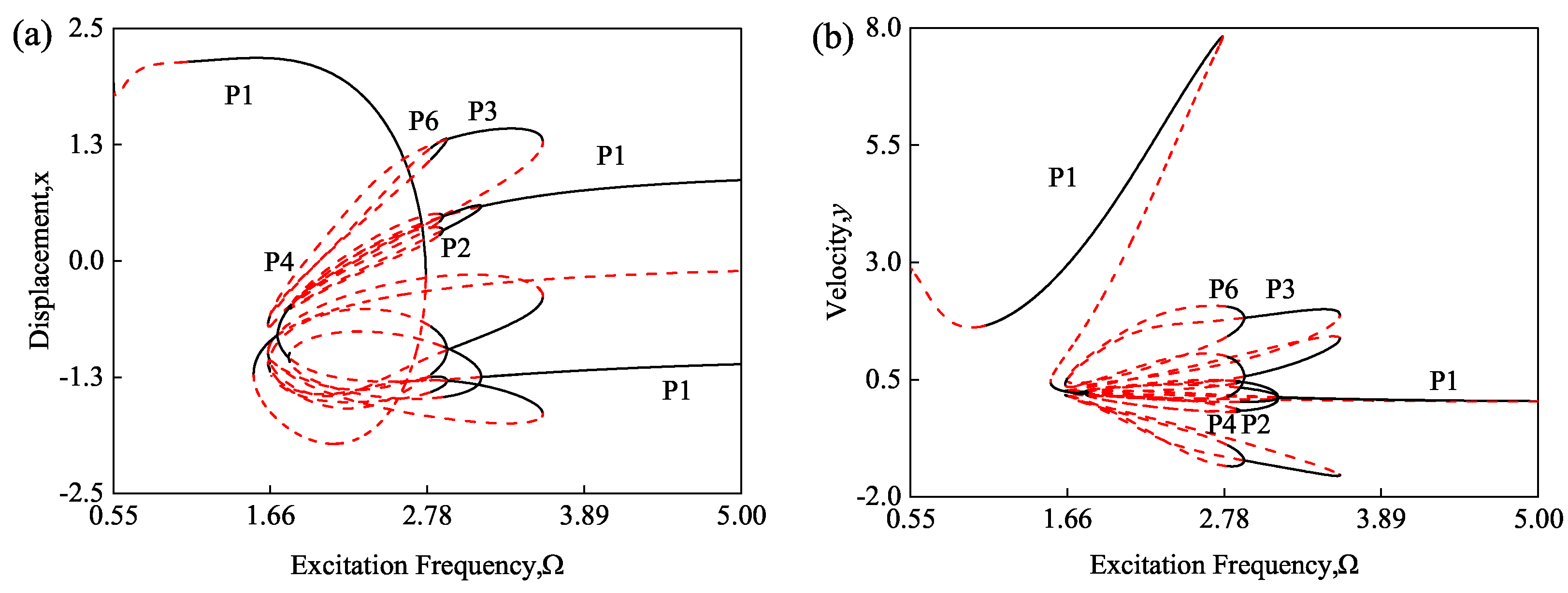
Setting system parameters , , the bifurcation analysis can be obtained via the discrete mapping method. The global bifurcation diagram of the Duffing oscillator is shown in Figure 1. The excitation frequency is calculated from 0.55 to 5. “SN” and “PD”, respectively, represent saddle-node and period-doubling bifurcations. The stable motion is depicted by the black solid line, whereas the red dashed line illustrates unstable solutions that are unattainable through conventional numerical methods. Through the implicit mapping algorithm, a comprehensive overview of both stable and unstable periods of the Duffing oscillator is presented. In implicit mapping method, instability refers to higher-order period existence. And the eigenvalues provide the bifurcation characteristics in Duffing oscillator motion. From Figure 1, the complete bifurcation tree from period-1 to chaos could be predicted by analyzing the periodic motions of the Duffing oscillator. Period-1, 2, 4, and period-3, 6 are labeled P1, P2, P4, and P3, P6, respectively.

Figure 1.
A global view of bifurcation trees varying with excitation frequency : (a) node displacement x; (b) node velocity y.
To clearly describe the periodic motion, the bifurcation trees and points of periods 1, 2, and 4 are depicted in Figure 2. From Figure 2, it can be observed that period-1 motion exists in the range of (0.55, 5.00). The stable period-1 motion is (0.55, 0.5577), (1.07, 2.76), (1.54, 1.79), (3.16, 5.00), while the unstable period-1 motion takes place in the range of (0.5577, 1.07), (1.54, 2.76), (1.71, 5.00). There are many interlaced periodic lines indicating different periodic behaviors of the system. The corresponding saddle-node bifurcations in the multiple solution ranges occur at = 0.5577, 1.55, 1.71, 1.79, 2.76, where there exists a jumping phenomenon. Additionally, at = 3.16, a period-doubling bifurcation leads to a transition from period-1 to period-2 motion with excitation frequency decrease. The periodic line of period-2 motion has two limit circles. The stable motion range of period-2 is (1.79, 1.80), (2.89, 3.16), while the unstable motion range is (1.80, 2.89). The system has period-doubling bifurcations at = 1.80 and = 2.89, respectively. Through the two period-doubling bifurcation points, period-2 undergoes a transition from stable to unstable and then back to stable. At = 2.89, period-doubling bifurcation appears and then the Duffing enters period-4 motion from period-2 motions with excitation frequency decrease. Period-4 motion is characterized by the presence of four limit circles within the range of (1.80, 2.89), with period-doubling bifurcations occurring at = 2.85 and = 2.89. The system exhibits a transition in stability as it moves through these bifurcation points, showcasing the complexity and dynamics of the periodic motion in the system.
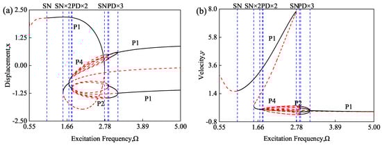
Figure 2.
A zoomed view of bifurcation trees (period-1 motions to period-4 to chaos): (a) node displacement x; (b) node velocity y.
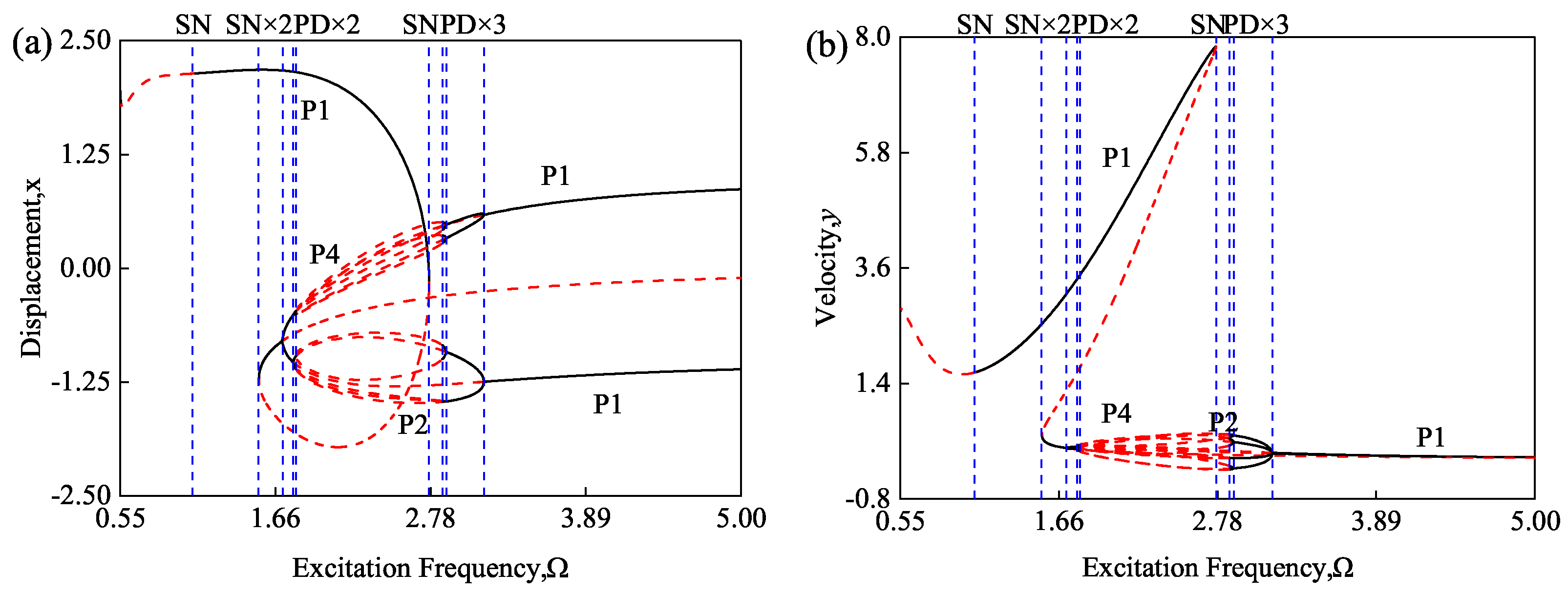
The bifurcation trees and points of period-3 to period-6 motion are depicted in Figure 3. Period-3 motion can be observed in (1.647, 3.596). The stability of period-3 motion is categorized into two areas: (1.647, 1.65) and (2.79, 3.596) for the stable motion; (1.65, 2.79) and (1.647, 3.596) for the unstable motion. In period-3 motion, there are mainly three mutually influencing periodic lines. The occurrence of four saddle-node bifurcations in period-3 motion happens at = 1.647, 1.65, 2.92, 3.595. Additionally, at = 2.92, it is still period-3 motion despite there being six periodic orbits. When = 2.79, a period-doubling bifurcation occurs, leading the system to transition from period-3 to period-6 motion as the excitation frequency decreases. The stable motion for period-6 is in the range of (2.779, 2.79). The unstable motion can be observed in the range of (1.66, 2.779). The system has a saddle-node bifurcation point at = 1.66. There are period-doubling bifurcations at = 2.779, 2.79.

Figure 3.
A zoomed view of bifurcation trees (period-1 motions to period-4 to chaos): (a) node displacement x; (b) node velocity y.
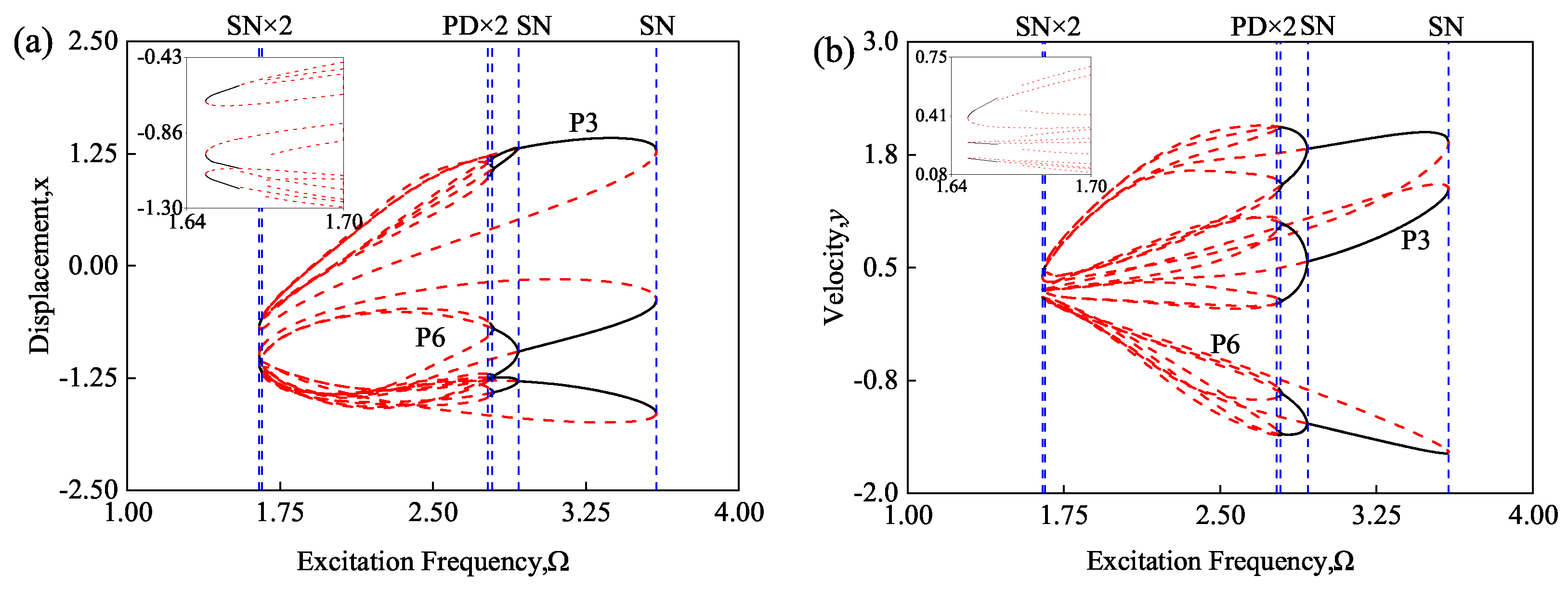
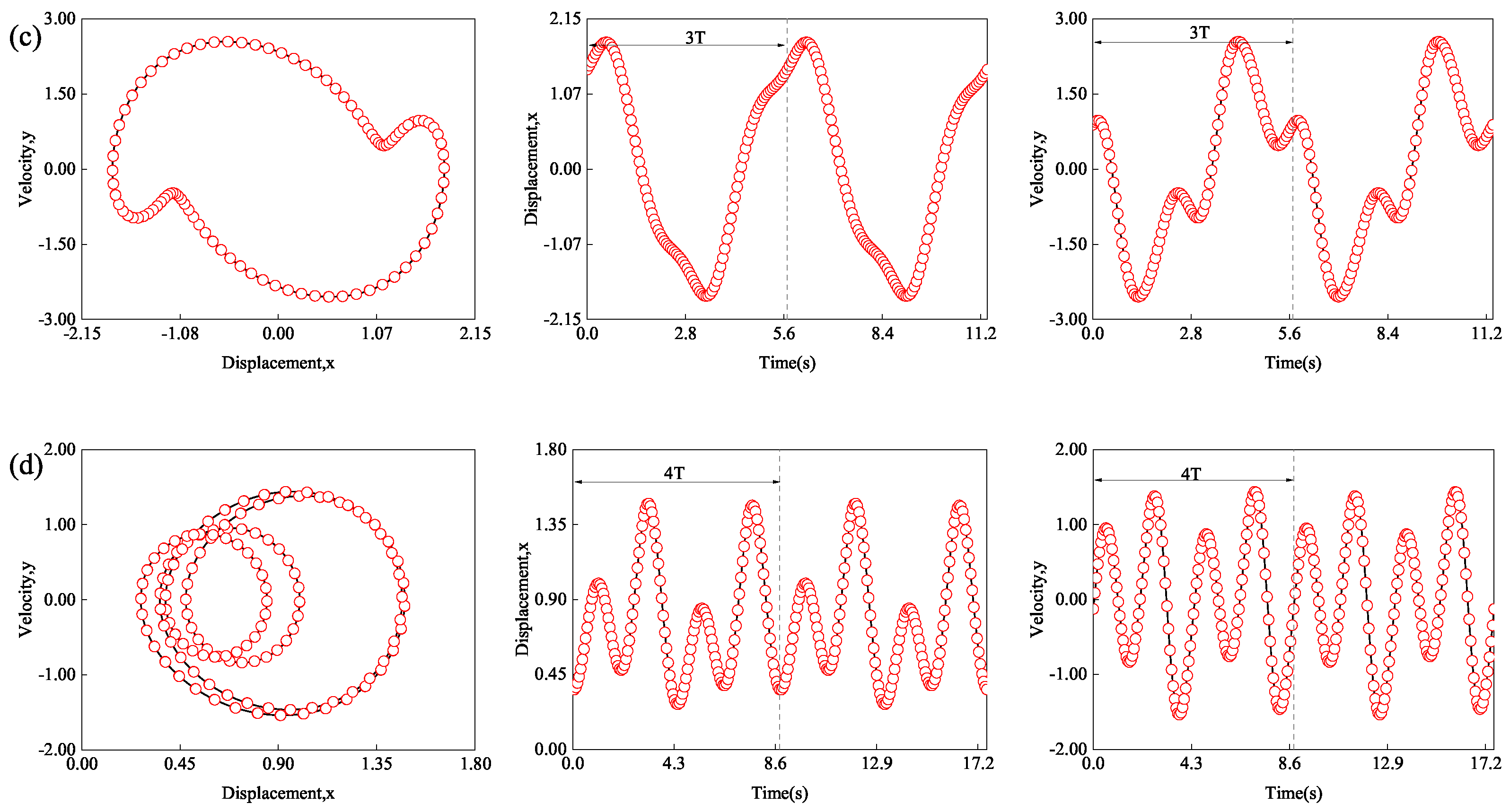
The phase trajectories and wave-forms of stable periodic motions are shown in Figure 4. From the graph, the trajectory of period-1 has a circle, and the wave forms have one peak in one period. There are two circles in the trajectory of period-2 motion, with the slowly changing part having a smaller orbit and the rapidly changing part having a larger orbit. Correspondingly, the wave-forms have two peaks in one period. The phenomenon is also appropriate for period-4 motion. For period-3 motion, only one circle is observed because there is a low rate of change for the displacement x.
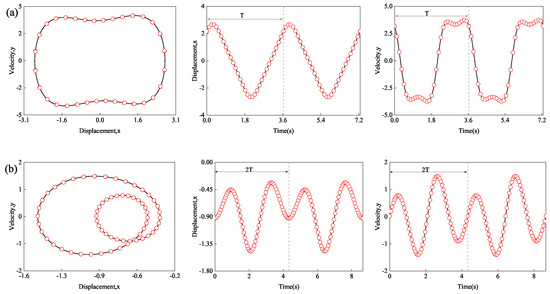

Figure 4.
Phase trajectories and waveforms: (a) stable periodic motions; period-1 with = 1.73; (b) stable periodic motions; period-2 with = 2.9; (c) stable periodic motions; period-3 with = 3.309; (d) stable periodic motions; period-4 with = 2.8606.
3.2. Periodic Motions of Duffing Oscillator with Excitation Amplitude
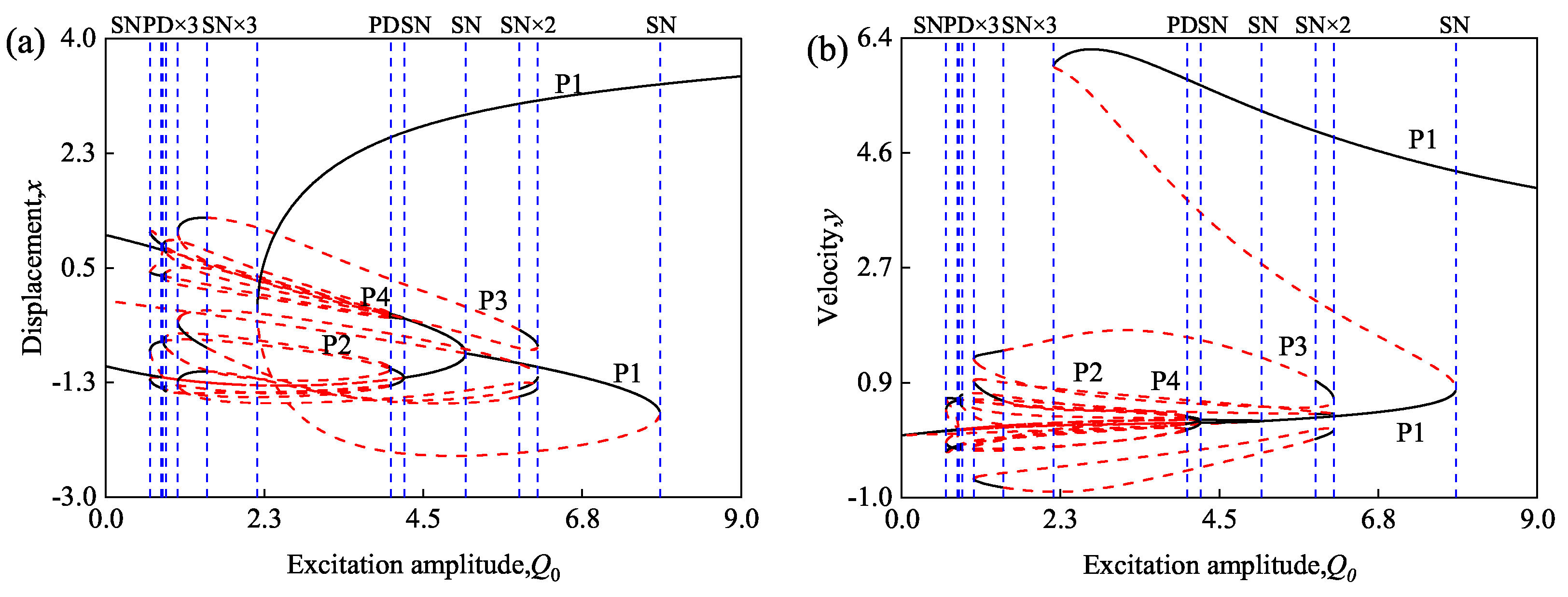
Given system parameters = 2.4 and = 0.3, Figure 5 shows the predicted trends of node displacement x and velocity y in relation to changes in excitation amplitude . In Figure 5, the predictions of a bifurcation tree completely transitioning from period-1 to chaos are illustrated. The period-1, 2, 4, and 3 motions are labeled P1, P2, P4, and P3, respectively. The period-2 motion arises from the period-doubling bifurcation of period-1 motion, and period-4 motion results from the period-doubling bifurcation of period-2 motion.

Figure 5.
A global view of bifurcation trees varying with excitation excitation amplitude : (a) node displacement x; (b) node velocity y.
Period-1 motion is found within the range of (0, 9.0). Stable period-1 occurs when (0, 0.79), (4.23, 7.85), (2.15, 9.0), while unstable period-1 motion takes place within (0.79, 4.23), (2.15, 7.85), (0, 5.10). As shown in Figure 5, there are many interacting periodic orbits in the bifurcation tree. The corresponding saddle-node bifurcations in the multiple solutions are at = 4.23, 5.10, where there exists a jumping phenomenon. Furthermore, period-doubling bifurcations are observed at = 4.23, 5.10. At = 5.10, through a saddle-node bifurcation, the stable periodic orbit splits while the excitation amplitude decreases, but the periodic motion is still period-1. The stable period-2 motion takes place within the range of (0.63, 0.83), (4.04, 4.23), while the unstable range is within (0.82, 4.04). At the bifurcation points , a shift from stable to unstable motion occurs and then goes back to stable motion, signifying a transformation in the behavior of the system. Additionally, at , the system transitions from period-2 motion to period-4 motion, where the phase trajectory encompasses four circles within the range of . The stable period-4 motion is observed within , while unstable motion falls within the interval of . These findings highlight the complex dynamics and transitions exhibited by the system under varying values of .
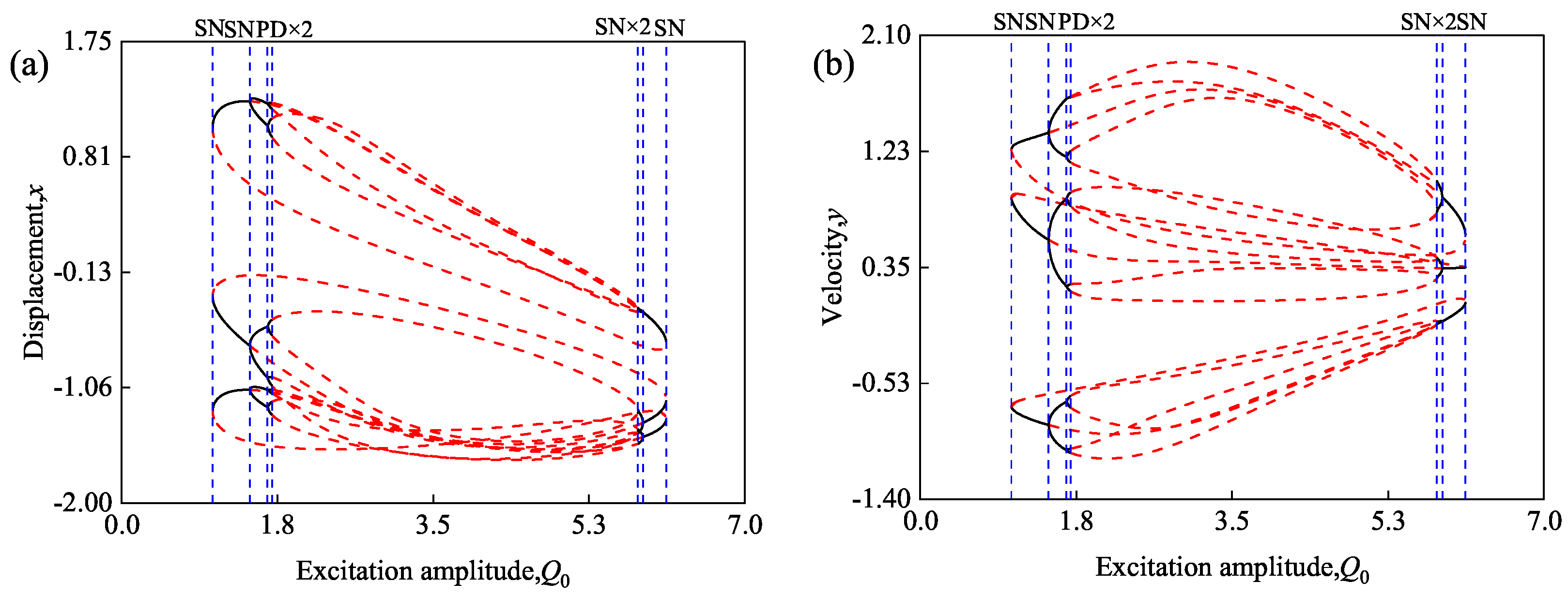
The movements of period-3 and 6 are depicted in Figure 6. Period-3 motion occurs within the interval of (1.02, 6.12). Period-3 exhibits stability within the range of (1.02, 1.64), (5.86, 6.12), while instability is observed in the intervals of (1.02, 6.12), (1.44, 5.86), (1.64, 5.86). There are three limit circles associated with the periodic trajectory of period-3. Five saddle-node bifurcations in period-3 are located at = 1.02, 1.44, 5.8, 5.86, 6.12, respectively. The period-doubling bifurcation points are = 1.64, 1.69. Furthermore, at = 1.44, the Duffing model is still in period-3 motion, although the periodic orbit splits into six lines here. The system enters period-6 motion from period-3 motion with an excitation amplitude decrease at = 2.80. The stable period-6 motion range is (1.64, 1.69), while the range for unstable motion is (1.69, 2.80).
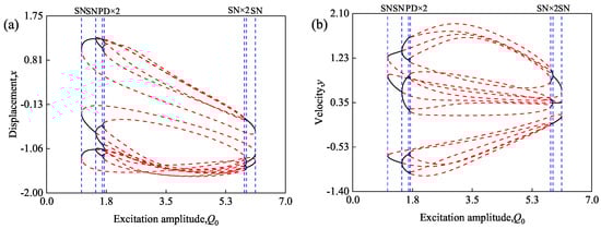
Figure 6.
A zoomed view of analytical prediction of bifurcation trees (period-1 motions to period-4 to chaos) (a) node displacement x; (b) node velocity y.
4. Periodic Transformation with the Excitation Amplitude and Frequency
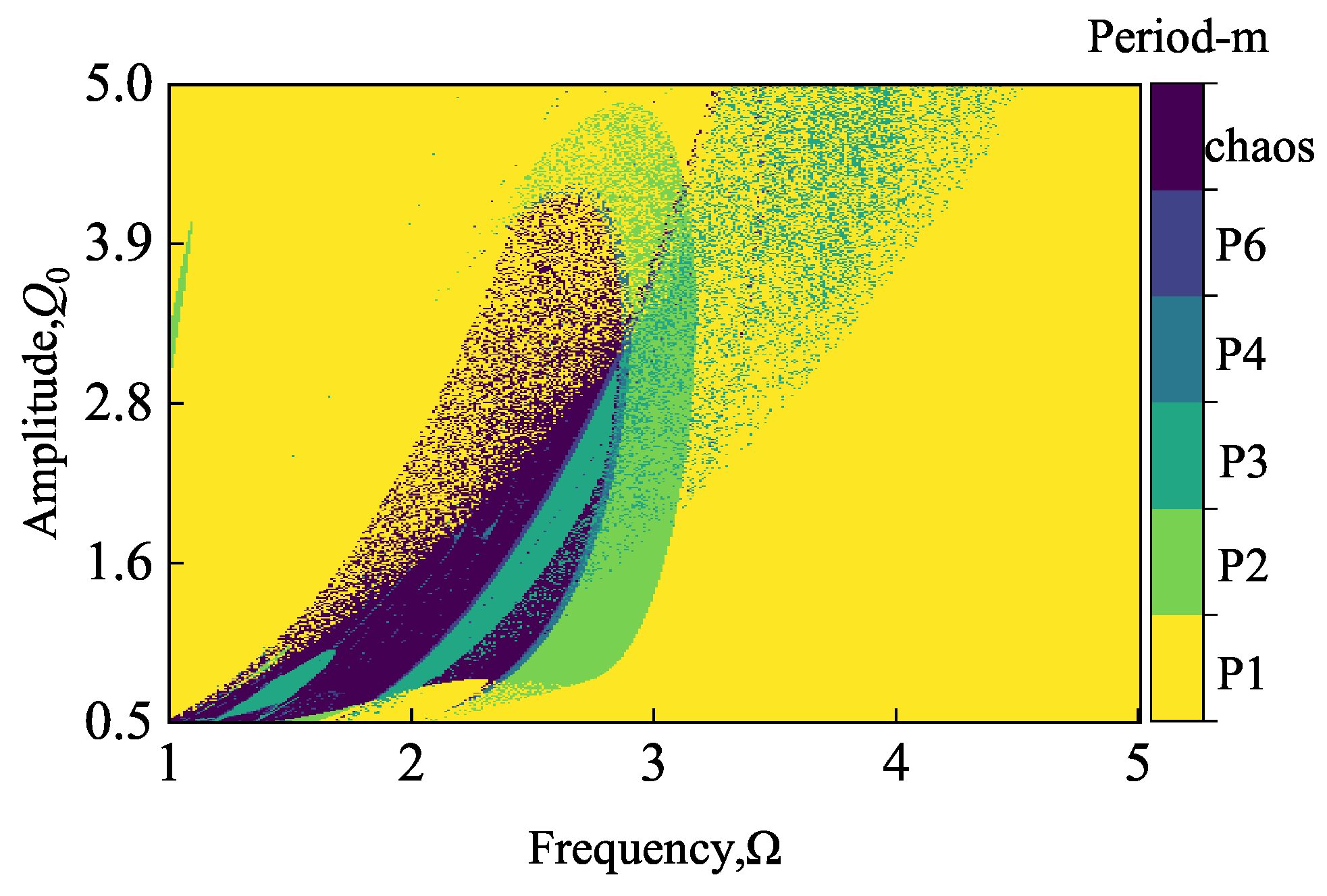
Figure 7 is a dual-parameter map which describes the period transformation of a typical Holmes–Duffing oscillator with the excitation amplitude (0.5, 5) and frequency (1, 5). A clear and accurate evolution of periodic motion and chaotic processes is provided in Figure 7. The Duffing oscillator is predominantly in period-1 motion, with high-period motion occurring at lower frequencies. It is notable that period-1 and period-2 motion are closely neighboring. Additionally, the adjacent relation exists between period-2 and period-4 motion, and is also appropriate for period-3 and period-6 motion. The periodicity and chaos shown in Figure 7 are consistent with the inferences illustrated in Figure 1 and Figure 5.
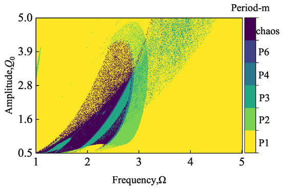
Figure 7.
Dual-parameter map (, ).
In addition, there are multiple regions where different periodic motions intertwine and intersect. For example, the alternating phenomenon between yellow and green indicates the simultaneous presence of period-1 and period-3 motion when (3.40, 4.29). Similarly, when (2.91, 3.17), period-2 and period-3 appear alternately. The periodic entanglement could also be observed in Figure 1 and Figure 5 under the same excitation conditions shown in Figure 7. These results are due to the complex dynamic characteristics of the Duffing model. Even with the same system parameters, the periodic states depend on the initial values and . The periodic states vary with the initial values. The dual-parameter map could help to understand the influence of excitation conditions on the periodicity of the Duffing oscillator and meet the requirements of FPGA circuit parameters selection.
5. Implementation of Duffing Circuit Based on FPGAs
In this section, an FPGA circuit is designed to simulate the periodic activity of Duffing oscillators and verify the periodic characteristics under the above parameters. The semi-analytic method is used to accurately judge the state and bifurcation point of the model, but it is not easy to implement in the FPGA circuit because of its large computation amount. The forward Euler method requires fewer resources and has a faster response time. The Euler method is used to discretize the dynamics equations of the Duffing model as follows:
In Equation (11), and are discrete values of state variables at the current moment, , are discrete values of state variables at the next moment, and is the integration step size. is the system parameter, and is the driving force signal. Due to the lack of direct support for decimal and differential operations in FPGA hardware, we utilize single-precision floating-point numbers in accordance with the IEEE-754 standard [26] for our computations.
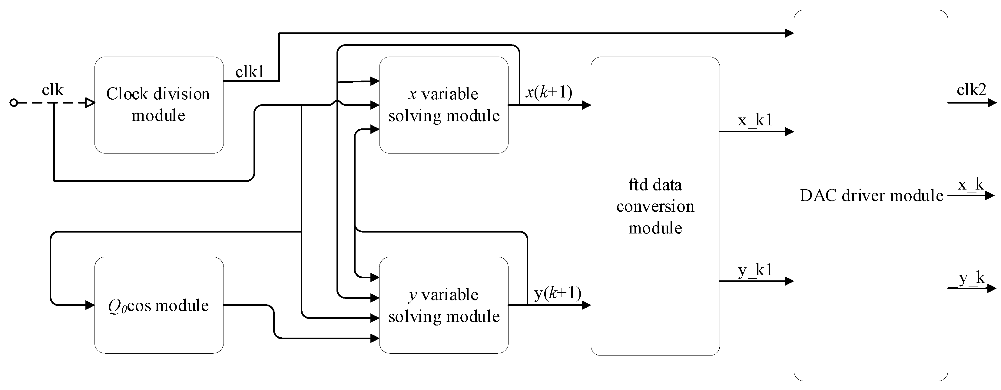
The model block diagram of the Duffing model in FPGAs is shown in Figure 8. In Figure 8, the function of the clock division module is to divide the external input clock (clk) into clk1 clock signals by internal count. The clk1 is connected to the DAC driver module as the clock signal for the DAC chip; clk is the clock signal for the variable-solving module and module, respectively. The module is used to store cos values in a ROM register and continuously provide the corresponding cos value based on the clock signal. The value of the cosine function is calculated according to the set integration step. Then, the pre-calculated internal driving force of the Duffing oscillator is converted into a .mif file and stored in the fixed-size ROM. This allows for quick access through the look-up table method. Then, the variable value is entered into the y variable-solving module for solving.The ftd data conversion module receives 32-bit data and from the variable-solving module as input. Then, it performs appropriate bit-width conversion, converting the 32-bit data into 14-bit data x_k1 and y_k1, often including truncation to ensure the output data range aligns with the range of the DAC chip. The task of the DAC driver module is to provide the clock signal for the DAC chip and output the variable value. The variable-solving module realizes the solution of Equation (11). In the design, the two state variables and are solved separately. The state variables at the current moment and are fed back to the variable-solving module as input for solving the state variable value at the next moment.

Figure 8.
Duffing digital model block diagram.
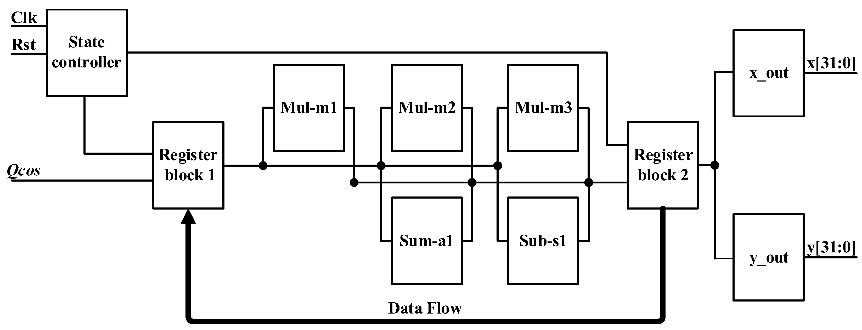
In the computation module shown in Figure 9, three floating-point multipliers, one floating-point summator, and one floating-point subtractor serve as shared resources for all data operations. The solution for the discrete system is structured into five steps. Given that the 32-bit multiplier requires substantial area, we store data in registers after each calculation step. This approach enhances the module’s maximum operating frequency by ensuring data stability and optimizing pipeline efficiency. The designed circuit model was simulated by Modelsim SE 10.5. The Modelsim simulation result of Duffing at period-1 motion is shown in Figure 10.

Figure 9.
The computation block diagram of Duffing.
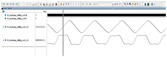
Figure 10.
Modelsim simulation result of Duffing.
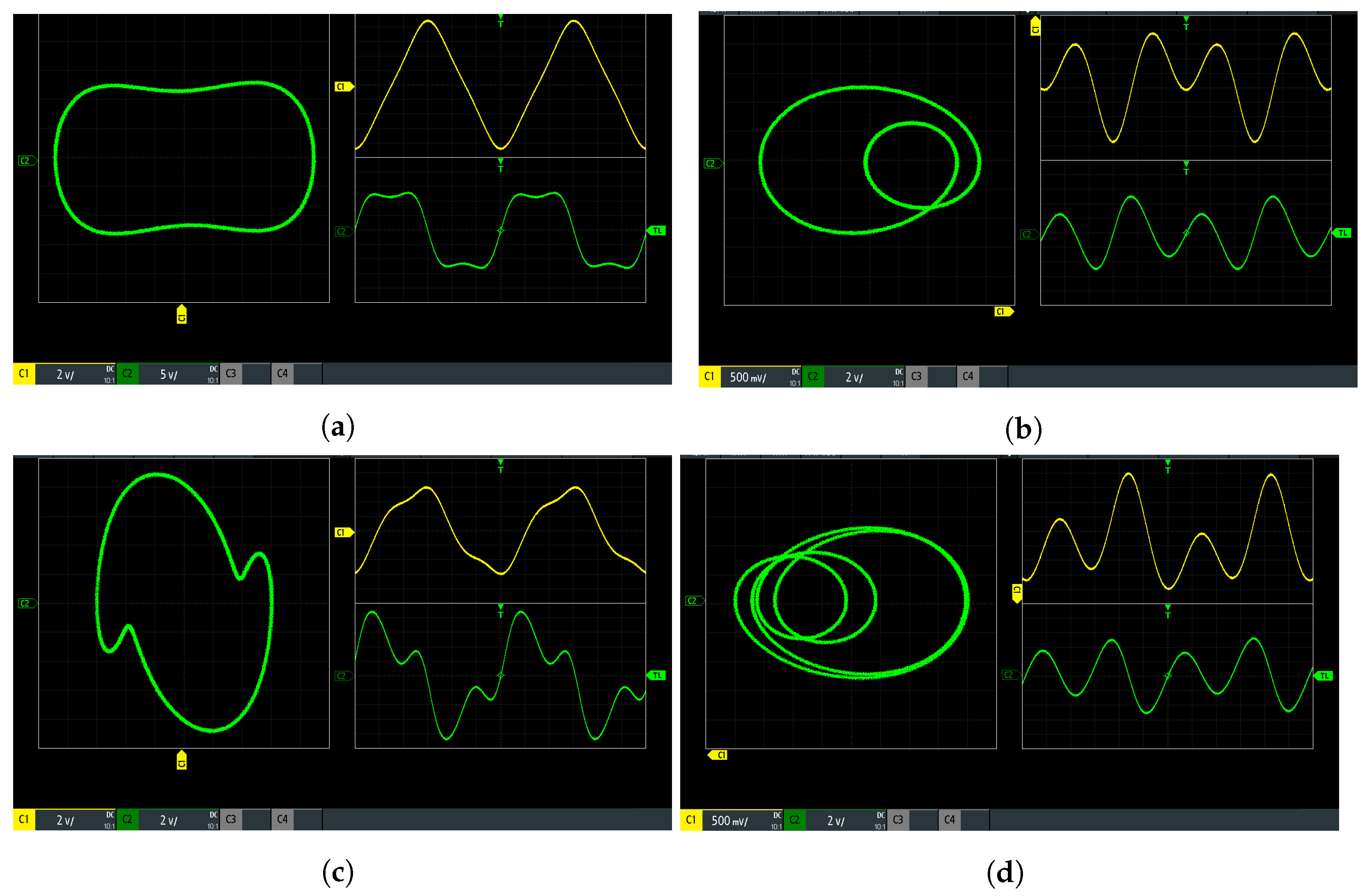
We constructed a validation environment for the Duffing system as seen in Figure 11. The DAC module of the Duffing chaotic digital system is connected to an oscilloscope via a dual-ended cable with BNC connectors. The output of state variable x and y are connected to the oscilloscope. The screen of the oscilloscope shows the x-y phase trajectories and wave-forms of the Duffing system. According to the periodic phenomenon shown in Figure 7, we adjust the parameters of external amplitude and frequency to observe various periodic motions. The four types of phase trajectories and wave-forms of periodic motions are shown in Figure 12. Under different parameter conditions, Duffing oscillators have different periodic motion states.
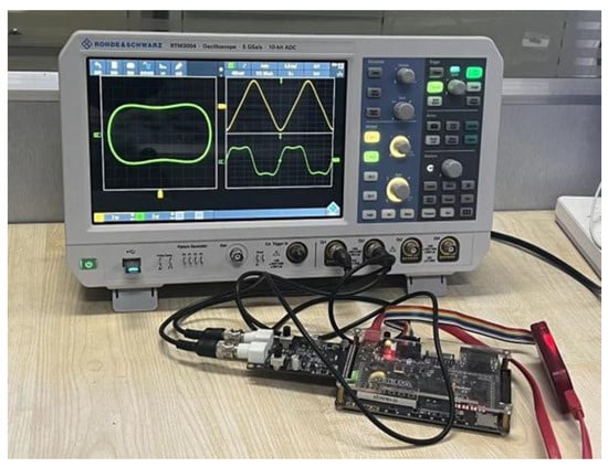
Figure 11.
FPGA implementation of Duffing model.
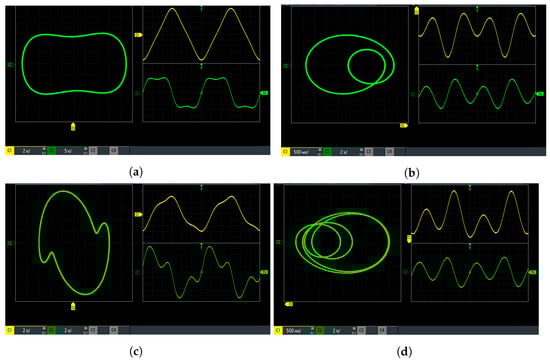
Figure 12.
x-y phase trajectories and wave-forms of the Duffing system: (a) period-1 motion with = 1.73, = 2.8; (b) period-2 motion with = 2.9, = 2.8; (c) period-3 motion with = 3.309, = 2.8; (d) period-4 motion with = 2.8606, = 2.8.
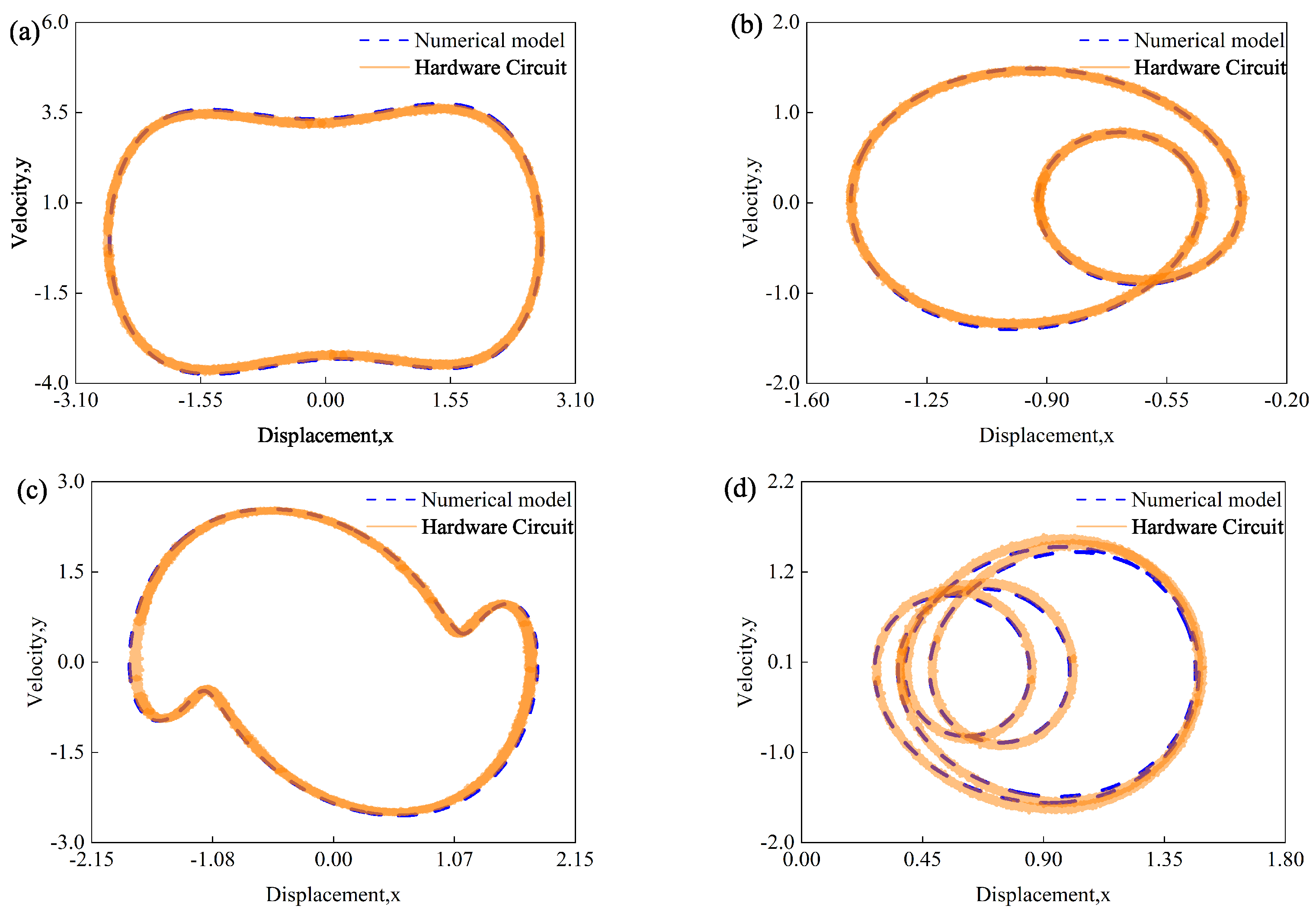
To achieve a comprehensive assessment of experimental outcomes, we extract the oscilloscope data as the results of the hardware circuit experiment. A comparative analysis between hardware circuit results and numerical results is performed, as depicted in Figure 13. The results of the FPGA hardware circuit are represented by the solid curves, while the numerical model is depicted by the dashed curves. The results show that there is a favorable agreement between the experimental outcomes of the FPGA hardware setup and the theoretical predictions from simulation. According to Equations (12) and (13), the difference value and difference rate can be calculated.
where refers to the value of the hardware circuit and is the value of the numerical model. The difference value of period-1 motion under the conditions of = 1.73, Q = 2.8 is shown in Table 1. The difference is small and the error rate under different is less than 5%, as shown in Table 2 (in the range of ). The results indicate that the designed hardware circuit can simulate the numerical model well.
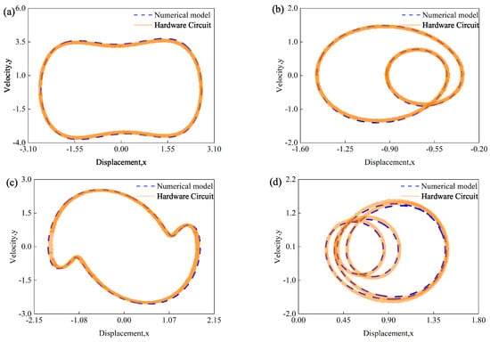
Figure 13.
Duffing phase trajectories of period motion for numerical model and hardware circuit: (a) period-1 motion with = 1.73, = 2.8; (b) period-2 motion with = 2.9, = 2.8; (c) period-3 motion with = 3.309, = 2.8; (d) period-4 motion with = 2.8606, = 2.8.

Table 1.
The difference values between numerical model and hardware circuit.
Table 2.
Error rate of numerical model and hardware circuit.
The phase trajectories of the theoretical and circuit methods are nearly identical, exhibiting only minor deviations. These differences arise from rounding errors inherent in floating-point arithmetic and the varying accuracy levels between the Euler method and the semi-analytic method. This means that the two results are approximately consistent in the hardware implementation. This agreement between the two sets of results enhances the validity and reliability of this study’s findings.
6. Conclusions
This study analyzes the bifurcation trees of Duffing oscillators and designs a FPGA hardware circuit to implement the function of the model. Some periodic characteristics are obtained from the bifurcation diagrams varying with the excitation frequency and excitation amplitude. Periodic-doubling bifurcation leads to a change in the periodicity of periodic motion. The saddle-node bifurcation changes stability. The number of branch lines does not correspond to the number of periods. However, the number of peaks in the wave-forms is consistent with the number of periods. The Duffing model is more easily affected by the initial value when the parameters are fixed. A dual-parameter map is investigated closely to satisfy the need of parameter selection for FPGA circuits. The phenomenon of various periods intersecting is studied to set the parameter of the FPGA circuit, which could avoid the circuit system entering unstable regions. Compared with the numerical solution, the hardware circuit exhibits good agreement with the semi-analytical findings. There are minor errors due to the fact that data conversion processes in FPGAs could influence the precision of the hardware circuit. The research exhibited new perspectives on Duffing models and nonlinear hardware circuits, and is of great significance in practical engineering problems such as rotating machinery, fault diagnosis, and signal detection. Our findings provide a reference for their implementation
Author Contributions
Conceptualization, Y.L.; Methodology, W.L.; Software, W.L.; Formal analysis, T.M.; Data curation, Z.Y.; Writing—original draft, Z.Y.; Writing—review & editing, T.M.; Supervision, Y.L. All authors have read and agreed to the published version of the manuscript.
Funding
This research received no external funding.
Data Availability Statement
The original contributions presented in the study are included in the article, further inquiries can be directed to the corresponding author.
Conflicts of Interest
The authors declare no conflict of interest.
References
- Chen, Q.; Fischer, M.; Nojiri, Y.; Renger, M.; Xie, E.; Partanen, M.; Pogorzalek, S.; Fedorov, K.G.; Marx, A.; Deppe, F.; et al. Quantum behavior of the duffing oscillator at the dissipative phase transition. Nat. Commun. 2023, 14, 2896. [Google Scholar] [CrossRef] [PubMed]
- Arun, K.; Tom, D.; Domenico, S. Review of polynomial chaos-based methods for uncertainty quantification in modern integrated circuits. Nat. Commun. 2018, 7, 30. [Google Scholar]
- Wang, S.; Lu, B. Detecting the weak damped oscillation signal in the agricultural machinery working environment by vibrational resonance in the duffing system. J. Mech. Sci. Technol. 2022, 36, 5925–5937. [Google Scholar] [CrossRef]
- Li, G.; Xie, R.; Yang, H. Study on fractional-order coupling of high-order Duffing oscillator and its application. Chaos Solitons Fractals 2024, 186, 115255. [Google Scholar] [CrossRef]
- Mohamed, B.; Iqbal, J.; Zoubir, D. A new nonlinear duffing system with sequential fractional derivatives. Chaos Solitons Fractals 2021, 15, 111247. [Google Scholar]
- Papangelo, A.; Fontanela, F.; Grolet, A.; Ciavarella, M.; Hoffmann, N. Multistability and localization in forced cyclic symmetric structures modelled by weakly-coupled duffing oscillators. J. Sound Vib. 2018, 440, 202–211. [Google Scholar] [CrossRef]
- UriosteguiLegorreta, U.; Tututi, E.S. Numerical study on synchronization in the rayleigh–duffing and duffing oscillators. Int. J. Mod. Phys. C 2023, 34, 2350122. [Google Scholar] [CrossRef]
- Reis Eduardo, V.M.; Savi Marcelo, A. Spatiotemporal chaos in a conservative duffing-type system. Chaos Solitons Fractals 2022, 165, 112776. [Google Scholar] [CrossRef]
- He, Y.; Liu, Y.; Zhang, H. Numerical and electrical simulation of a hindmarsh-rose neuron model. J. Vib. Test. Syst. Dyn. 2022, 6, 329–341. [Google Scholar]
- Albert, C.; Luo, J. Discretization and Implicit Mapping Dynamics; Springer: Berlin/Heidelberg, Germany, 2015. [Google Scholar]
- Albert, C.; Luo, J. Periodic flows to chaos based on discrete implicit mappings of continuous nonlinear systems. Int. J. Bifurc. Chaos 2015, 25, 1550044. [Google Scholar]
- Guo, Y.; Albert, C.; Luo, J. On complex periodic motions and bifurcations in a periodically forced, damped, hardening duffing oscillator. Chaos Solitons Fractals 2015, 81, 378–399. [Google Scholar] [CrossRef]
- Guo, Y.; Albert, C.; Luo, J. Periodic Motions to Chaos in Duffing Oscillator via Discretization Technique; Springer International Publishing: Cham, Switzerland, 2016; pp. 259–276. [Google Scholar]
- Albert, C.; Luo, J.; Xing, S. Bifurcation trees of period-3 motions to chaos in a time-delayed duffing oscillator. Nonlinear Dyn. 2017, 88, 2831–2862. [Google Scholar]
- Liu, Y.; Zhang, H.; He, Y.; Xu, Y. Independent continuous periodic firing series to chaos in the 3-d hindmarsh–rose neuron circuit. Int. J. Non-Linear Mech. 2023, 155, 104454. [Google Scholar] [CrossRef]
- Xu, Y.; Albert, C.; Luo, J. Paired asymmetric periodic oscillations in a pair of first-order asymmetric nonlinear circuit systems. Mech. Syst. Signal Process. 2022, 171, 108810. [Google Scholar] [CrossRef]
- Zhang, X.; Min, F.; Dou, Y.; Xu, Y. Bifurcation analysis of a modified fitzhugh-nagumo neuron with electric field. Chaos Solitons Fractals 2023, 170, 113415. [Google Scholar] [CrossRef]
- Mohamed Sara, M.; Sayed Wafaa, S.; Said Lobna, A.; Radwan Ahmed, G. Reconfigurable fpga realization of fractional-order chaotic systems. IEEE Access 2021, 9, 89376–89389. [Google Scholar] [CrossRef]
- Rui, Z.; Min, F.; Dou, Y.; Ye, B. Switching mechanism and hardware experiment of a non—Smooth rayleighduffing system. Chin. J. Phys. 2023, 82, 134–148. [Google Scholar] [CrossRef]
- Li, B.; Xu, Y.; Shi, H.; Xue, W. Fpga realization of duffing chaotic oscillator based on runge-kutta algorithm. In Proceedings of the 2017 2nd International Conference on Automation, Mechanical Control and Computational Engineering (AMCCE 2017), Beijing, China, 25–26 March 2017; pp. 308–311. [Google Scholar]
- Li, G.; Zhao, K.; Yang, H. A new method for detecting line spectrum of ship-radiated noise based on a new double duffing oscillator differential system. Indian J. Geo-Mar. Sci. 2020, 49, 34–43. [Google Scholar]
- Yan, S.; Sun, X.; Wang, E.; Song, J.; Cui, Y. Application of Weak Signal Detection Based on Improved Duffing Chaotic System. J. Vib. Eng. Technol. 2023, 11, 3057–3068. [Google Scholar] [CrossRef]
- Rajagopal, K.; Khalaf Abdul Jalil, M.; Wei, Z.; Viet-Thanh, P.; Alsaedi, A.; Hayat, T. Hyperchaos and Coexisting Attractors in a Modified van der Pol-Duffing Oscillator. Int. J. Bifurc. Chaos 2019, 29, 1950067. [Google Scholar] [CrossRef]
- Xu, Y.; Wang, M.; Lu, D.; Zandigohar, M. Construction of complex high order subharmonic vibrations in a nonlinear rotor system I: Eigenvalue dynamics and prediction. J. Sound Vib. 2021, 582, 118439. [Google Scholar] [CrossRef]
- Xu, Y.; Chen, Z.; Albert, C.; Luo, J. Period-1 motion to chaos in a nonlinear flexible rotor system. Int. J. Bifurc. Chaos 2020, 30, 2050077. [Google Scholar] [CrossRef]
- IEEE-754; IEEE Standard 754 Floating Point Numbers. IEEE: New York, NY, USA, 1985.


Disclaimer/Publisher’s Note: The statements, opinions and data contained in all publications are solely those of the individual author(s) and contributor(s) and not of MDPI and/or the editor(s). MDPI and/or the editor(s) disclaim responsibility for any injury to people or property resulting from any ideas, methods, instructions or products referred to in the content. |
© 2024 by the authors. Licensee MDPI, Basel, Switzerland. This article is an open access article distributed under the terms and conditions of the Creative Commons Attribution (CC BY) license (https://creativecommons.org/licenses/by/4.0/).