Integrated Spatio-Temporal Graph Neural Network for Traffic Forecasting

Abstract

This research introduces integrated spatio-temporal graph convolutional networks (ISTGCN), designed to capture complex spatiotemporal traffic data patterns. The proposed model integrates multi-layer graph convolutional networks (GCNs) to address dependencies in temporal and spatial traffic dynamics. Specifically, ISTGCN integrates graph convolutional layers and convolutional sequence learning layers within multiple spatiotemporal convolutional blocks. For capturing the temporal aspect, predictive graph modeling for road network traffic at particular time stamps is performed. To integrate the spatial information, graph convolution operations are applied. The proposed model was validated on real-life datasets, and the experimental results demonstrate that ISTGCN achieves significantly lower error values across key metrics—RMSE, MAE, and MAPE.

1. Introduction

In the rapidly evolving landscape of smart cities, transportation systems are pivotal in shaping urban life. Challenges arising from rapid urbanization, population growth, and complex traffic networks necessitate innovative solutions, especially in traffic forecasting. Spatiotemporal graph convolutional networks (GCNs) are critical for enhancing traditional methodologies by effectively modeling the dynamic and interconnected nature of urban traffic. GCNs leverage real-time data from traffic sensors, GPS, and public transportation systems, enabling precise and adaptive traffic predictions essential for smart cities. They support dynamic traffic management, optimize multi-model transportation systems, and enable scalable solutions that adapt to evolving urban environments. By integrating these models, city planners can make informed decisions, reduce congestion, and improve overall mobility, contributing to a smarter, more resilient urban infrastructure.

Deep learning has emerged as a cornerstone in advancing traffic forecasting research, yielding substantial advancements. Authors in [1] provide an in-depth examination of recent geospatial data-based traffic forecasting applications, introducing a novel framework that transforms geospatial data into images through sophisticated methodologies such as convolutional neural networks (CNNs) and residual networks. The simplicity and efficacy of their approach surpass traditional methods, as demonstrated in addressing the New York taxi pick-up/drop-off forecasting problem.

Graph neural networks (GNNs) have gained prominence in deep learning research, showcasing cutting-edge performance across diverse applications [2]. GNNs are particularly well suited for addressing traffic forecasting challenges due to their ability to capture spatial dependencies, often modeled using non-Euclidean graph structures. Leveraging such graph representations as inputs, in recent times, a numerous of GNN-based models have demonstrated remarkable effectiveness surpassing traditional techniques in endeavors like forecasting road traffic flow and speed. Standout examples include the diffusion convolutional recurrent neural network (DCRNN) [3] and Graph WaveNet [4] models. Moreover, the GNN-based methodology has expanded to embrace various transportation modes, employing diverse graph formulations and models.

There is a burgeoning body of literature leveraging GCNs for smart city traffic forecasting, as evidenced by studies [5] demonstrating the efficacy of GCNs in capturing spatiotemporal dependencies for enhanced predictions. Researchers in [6] utilize traffic sensors and explore the integration of Internet of Things (IoT) devices to enrich traffic prediction, showcasing the synergy between IoT data and GCNs. The emphasis on real-time public transportation records, as shown by authors in [7], aligns with research investigating the impact of real-time data streams on improving the responsiveness and accuracy of traffic forecasting models in smart city environments.

Accurate real-time traffic speed prediction is essential for developing intelligent and efficient transportation systems, critical for applications such as congestion avoidance, route navigation, and traffic monitoring. However, challenges persist in accurately predicting unbalanced flow patterns and navigating complex dynamic traffic environments.

In data-driven methodologies, traditional statistical and machine-learning models serve as foundational pillars. Autoregressive integrated moving average (ARIMA) and its derivatives have long been stalwarts in time-series analysis, rooted in classical statistics [8]. However, these models face limitations stemming from the assumption of stationarity in time sequences and the neglect of spatiotemporal correlations, constraining their ability to represent highly nonlinear traffic flow patterns. In recent years, machine learning techniques such as the support vector machine (SVM), k-nearest neighbors algorithm (KNN) and neural networks (NNs) have emerged as formidable contenders in traffic prediction tasks, offering the potential for improved prediction accuracy and more intricate data modeling capabilities. In contemporary traffic analysis, deep learning methodologies have gained widespread adoption and demonstrated significant success across many tasks. Notable advancements include the utilization of deep belief networks (DBNs) [9] and stacked autoencoders (SAEs) [9].

It is well known that densely connected networks encounter challenges in jointly extracting spatial and temporal features from input data, particularly in scenarios with limited or absent spatial attributes. To address these challenges, the present research proposes novel strategies for effectively modeling traffic flow temporal dynamics and spatial dependencies. Our solution, integrated spatio-temporal graph convolutional networks (ISTGCN), integrates graph convolutional layers and convolutional sequence learning layers within multiple spatiotemporal convolutional blocks. This makes it a pioneering effort to apply purely convolutional structures to extract spatiotemporal features concurrently from graph-structured time series data in the context of traffic analysis.

Our contributions can be outlined as:

• Predictive graph modeling for road network traffic at particular time stamps.
• Applying graph convolution operations to integrate the spatial information.
• Integrated spatio-temporal graph convolutional network (ISTGCN) to capture the complex spatial and temporal dependencies inherent in the dataset.

This paper is structured as follows: Section 2 reviews our research in comparison with other relevant studies. Section 3 categorizes the traffic forecasting problem and outlines the methodology, covering predictive modeling for road networks and graph-based convolutional operations, proposed network architecture, and the discussion on extracting spatial and temporal features. Section 4 explains the experimental setup and discusses results and analysis. Finally, Section 5 concludes by addressing challenges and outlining future directions.

2. Related Work

The literature survey begins by exploring various traffic forecasting problems discussed in existing research. Initially, these problems are categorized based on the traffic state they aim to predict, such as traffic flow, speed, demand, and other related issues. These traffic problems are categorized by the level of traffic states: road-level, region-level, and station-level, each with distinct modeling needs to capture spatial dependencies. Road-level issues use sensor or GPS data mapped onto road networks via map-matching, viewing the network as a graph of numerous road segments connected by spatial proximity. Station-level issues involve metro or bus station topologies, with dependencies defined by transit routes. Region-level issues treat areas as graph nodes, with spatial dependencies influenced by factors like land use from points-of-interest data. In the context of smart cities, these modeling approaches can be further enhanced by integrating real time, enabling a comprehensive understanding of urban mobility patterns. By employing machine learning techniques within smart city infrastructures, traffic forecasting can leverage additional layers of information, such as weather conditions, event schedules, and demographic changes, resulting in more accurate predictions. This holistic approach addresses current traffic challenges and paves the way for sustainable urban planning and intelligent transportation systems that can adapt to the evolving needs of urban environments.

2.1. Traffic Problems

Traffic forecasts can predict flow, speed, and demand, categorized into road-level, region-level, and station-level. Road-level forecasts use sensor or GPS data on road networks to predict traffic flow [10]. Station-based issues concentrate on the layout of metro or bus stations, analyzing connectivity and passenger flow [11]. Region-level problems deal with larger areas, using nodes in a graph to represent regular or irregular regions and extracting spatial dependencies based on land use purposes. Each category requires specialized approaches to effectively model and understand the traffic patterns specific to its context.

2.2. Traffic Flow

Traffic flow, referring to the passage of vehicles through spatial units such as road segments or sensor points, holds pivotal importance for various applications, including traffic congestion management, traffic light optimization, and emissions reduction efforts [12].

This survey covers traffic flow problems at road, region, and station levels, each with unique challenges. Road-level issues involve traffic volumes and metrics like traffic flow and road origin–destination [13]. Region-level flow extends the analysis to traffic volume within defined city regions, categorized by transport mode, including taxi, bike, ride-hailing, and dockless e-scooter flows. Station-level flow focuses on traffic volume at physical stations like subway or bus stops, categorized by station type.

Despite the effectiveness of traffic sensors, data collection remains challenging due to the high deployment and maintenance costs associated with them. Alternative approaches, such as leveraging mobile and IoT devices like GPS sensors, offer potential solutions, albeit with data quality concerns [14]. Moreover, traffic light control introduces additional complexities, as signal timing changes can significantly impact traffic flow dynamics and relationships between road segments. Thus, understanding and mitigating these challenges is crucial for accurate traffic flow prediction and effective traffic management strategies.

2.3. Traffic Demand

Forecasting traffic demand is crucial for the success of taxi and ride-hailing services, as it allows providers to efficiently allocate their limited resources to areas with high demand. This optimization not only improves service availability for passengers but also promotes the use of alternative transportation options, such as public transit, when there is a limited availability of taxis or ride-hailing vehicles. Traffic demand refers to the expected need for travel, which is not always fully met. For example, ride requests on ride-hailing platforms represent demand, but some of these requests may go unfulfilled due to a shortage of available drivers, especially during peak hours. Accurate predictions of travel demand are essential for the effective operation of vehicle scheduling systems, such as those used in online ride-hailing services [15]. However, in some instances, collecting potential travel demand from passengers proves challenging, leading to the use of transaction records as an approximation of demand [16]. Yet, this method may underestimate actual demand.

2.4. Advancements in Traffic Prediction Innovations and Solutions Using Graph Convolution Network

In the realm of smart cities, the intricate dynamics of traffic prediction present formidable challenges arising from spatio-temporal complexities and non-linear dynamics. Conventional methods grapple with high training costs and difficulty accurately capturing patterns, often neglecting correlations between distant roads. This paper addresses these challenges by introducing innovative solutions. One such solution is using 3D temporal graph convolutional networks (3D-TGCNs) for traffic prediction. Constructing road graphs based on time series similarity makes spatial information redundant. The models original 3D graph convolution approach markedly enhances accuracy, surpassing current baselines in empirical results [17]. Similarly, traffic forecasting encounters hurdles in capturing complex spatial-temporal correlations and non-linear patterns. Many existing approaches overlook direct spatial-temporal correlations, modeling these dependencies separately. The adaptive graph spatial-temporal transformer network (ASTTN) emerges as a breakthrough, drawing inspiration from the success of transformers. By directly modeling cross-spatial-temporal correlations using local multi-head self-attentions on an adaptive spatial-temporal graph, ASTTN excels in empirical results [18]. Traffic prediction becomes challenging in real-world applications due to dynamic spatiotemporal dependencies among traffic data. The adaptive spatio-temporal convolutional network (ASTCN) is introduced to tackle these challenges, incorporating a spatial graph learning module and an adaptive temporal convolution module. ASTCN consistently outperforms other models in extensive experiments on real-world traffic datasets [19]. Complex spatial-temporal correlations on road networks further complicate traffic forecasting. The DualGraph framework is introduced to address this limitation by simultaneously modeling traffic forecasting for nodes and edges. Empirical evaluations of public datasets demonstrate the effectiveness of the proposed method, especially in long-term predictions [20]. In fields like neurology and transportation, spatiotemporal forecasting faces complexity due to non-linearity, dynamic nature, and shifting road conditions. The dynamic temporal position observant graph neural network (DTPO-GNN) handles these challenges, incorporating positional awareness and spatial-temporal reliance on traffic flow. Controlled sample encoder–decoder architecture and two-way random walks make DTPO-GNN an efficient solution for accurate traffic forecasting in large-scale road networks [21].

Time series forecasting, crucial for applications like predicting solar plant energy output and traffic situations, is addressed with the transformer model. The study introduces convolutional self-attention and the LogSparse transformer to overcome insensitivity to local context and a memory bottleneck. Experimental results on synthetic and real-world datasets showcase the superiority of the proposed model [22].

Federated learning safeguards data privacy in intelligent transportation systems but often neglects topological information of transportation networks. The attention-based spatial-temporal graph neural networks (ASTGNN) model, integrated with a novel federated learning framework called FASTGNN, addresses this gap. The framework preserves topological information using a differential privacy-based approach, enabling local GNN-based models to access the global network for enhanced training [23].

Predicting traffic speed in intelligent traffic systems (ITSs) is challenging due to complex spatial-temporal correlations. The proposed GSTGCN, a deep-learning model for urban traffic speed prediction, effectively captures various correlations and external influences. Experimental results on real-world traffic datasets demonstrate GSTGCN’s superiority over state-of-the-art baselines [24].

In the realm of intelligent transportation systems, traffic forecasting relies on deep learning models, including graph neural networks (GNNs). This survey provides a comprehensive overview of GNN applications in traffic flow and vehicle speed forecasting [25].

The proposed CTFL framework utilizes a divide-and-conquer approach to address communication overhead in federated learning (FL) with GNN-based traffic forecasting models. By clustering clients based on local model parameters’ closeness and employing a two-step strategy for optimizing local models, CTFL showcases outstanding training efficiency and prediction accuracy in case studies on real-world datasets and GNN-based models [26].

Integrating multimodal data introduces challenges in terms of data complexity and volume. Efficiently managing and extracting insights from these data is pivotal for informed decision-making. Machine learning and data fusion techniques are highlighted as indispensable tools for unravelling meaningful patterns and optimizing urban services [27].

The synergy between machine learning and data fusion techniques becomes a cornerstone in the smart city landscape. Predictive machine learning models can forecast traffic congestion, optimize routing, and improve air quality. Energy management systems developed through machine learning contribute to reduced energy consumption and increased reliance on renewable sources [28].

GCNs, a specialized neural network tailored for graph-structured data, hold immense potential for smart cities. GCNs contribute to more accurate predictions and facilitate informed decision-making in dynamic urban environments by capturing spatial relationships and dependencies within urban networks [29]. The smart city concept employs advanced technologies such as graph convolutional networks (GCNs) to optimize urban infrastructure and enhance the quality of life for residents. GCNs are integrating graph convolutional networks into smart city frameworks for enhanced traffic analysis designed to effectively model complex relationships within spatially distributed data, making them particularly adept at traffic forecasting and urban mobility analysis.

In a smart city context, GCNs operate on graph-structured data where nodes represent various urban elements such as intersections, bus stops, or parking spaces and edges denote the spatial relationships between these nodes. This graph-based representation allows GCNs to capture intricate spatial dependencies [30], such as the influence of neighboring road segments on traffic flow at a given location. By utilizing adjacency matrices, GCNs can incorporate information from connected nodes, enhancing the model’s ability to predict traffic states like flow, speed, and congestion. Graph convolutional networks (GCNs) can be adapted to capture temporal dynamics by incorporating temporal convolutions or recurrent neural network (RNN) components, enabling them to process time-series data and improve accuracy in short-term traffic forecasting. Similarly, accurate traffic forecasting requires effectively capturing both long- and short-term patterns, which standard models often miss. The LSTTN framework addresses this gap by using a Transformer to learn key features from long traffic histories, enhancing predictions through an integration of long-term, periodic, and short-term trends, resulting in up to a 16.78% improvement over baseline models in long-term forecasting [31].

In a different context, LAMP in graph attention networks (GATs) improves node classification by learning the importance of neighboring nodes. However, in heterophilic graphs, dissimilar neighbors can cause a “Distraction Effect” (DE) that weakens performance. To mitigate this, CAT selectively removes distracting neighbors, boosting accuracy without altering the GAT architecture [32].

The application of GCNs in smart cities supports the development of adaptive traffic signal control systems that adjust in real time based on current traffic conditions. By analyzing real-time data from various sources, including traffic cameras and IoT devices, GCNs facilitate efficient routing algorithms that optimize traffic flow and reduce congestion.

Additionally, GCNs can assist in the identification of critical areas for infrastructure investment, enabling urban planners to make data-driven decisions. This capability not only contributes to improved traffic management but also promotes sustainability by encouraging the use of public transportation and reducing carbon emissions. Overall, GCNs play a transformative role in smart city initiatives, fostering enhanced connectivity, operational efficiency, and an improved urban living environment.

3. Methodology

The integrated spatio-temporal graph neural network (ISTGNN) model is designed to address complex traffic forecasting tasks by integrating spatio-temporal dependencies inherent in urban traffic data. The architecture leverages graph-based neural network layers, regression models, and sophisticated training routines to model traffic dynamics.

3.1. Predictive Modeling for Road Network Traffic

Predicting traffic presents a traditional hurdle in time-series forecasting, requiring the estimation of likely traffic data attributes (e.g., road capacity, vehicle movement) for the next H time intervals based on preceding M traffic observations. Mathematically, this involves determining.

$${\widehat{v}}_{t+1,}\dots ,v_{t+H }=\mathit{arg}\mathit{maxlog}\mathit{P}(v_{t+1 },\dots \dots v_{t+H }|v_{t-M+1},\dots \dots , v_t)$$

(1)

where v_t $ϵ R^n$ represents an observation vector of n road segment at t, with each element documenting historical data for a signal road segment. Our research uses a graph framework to characterize the traffic network, emphasizing structure traffic time series analysis. Each observation v_t can be conceptualized as a graph signal defined on an undirected or directed graph G, with weight w_i,j, as illustrated in Figure 1, where, at time t, the graph G_t = (V_t, E, W) comprises a finite set of vertices V_t corresponding to observation from n monitoring stations in a traffic network, E denotes a set of edges representing interconnection between stations, and W $ϵ R^{n\times n}$ signifies the weighted adjacency matrix G_t.

3.2. Graph-Based Convolutional Operations:

Presently, two fundamental approaches are being explored to generalize convolutional neural networks (CNNs) to accommodate structured data formats since utilizing a standard convolution technique, regular general graphs. One strategy involves broadening the spatial definition of convolution, which requires rearranging the vertices into specific grid-like configurations suitable for conventional convolutional operations. Another crucial avenue of exploration lies in graph-based convolutional operations, which leverage the inherent structure of graphs to perform convolutions directly on irregular data representations, such as road networks or social networks. This innovative approach allows for the incorporation of spatial dependencies and local connectivity patterns inherent in graph data, enabling more effective analysis and prediction tasks. The alternative approach operates within the spectral domain, leveraging graph Fourier transforms, often termed spectral graph convolution. This method applies convolutions in spectral domains, offering a promising avenue for graph convolution, particularly as subsequent studies have managed to reduce computational complexity from quadratic to linear. Based on spectral graph convolution principles, denoted as ‘*G’, it involves multiplying a signal x in Rⁿ with a kernel $\theta$, expressed as:

$$\theta \ast Gx=\theta \left(L\right)x=\theta \left(U\wedge U^T\right)x=\bigcup \theta \left(\Lambda \right)U^{T}x$$

(2)

where U is the graph Fourier basis matrix, L is the normalized graph Laplacian matrix, $\wedge$ represents the diagonal matrix of the eigenvalue of L, and $\theta \left(\Lambda \right)$ is diagonal matrix. This operation effectively filters graph signal x by convoluting it with the kernel $\theta$ using the graph Fourier transform $U^{T}x$.

3.3. Proposed Architecture: Integrated Spatio-Temporal Graph Neural Network

The integrated spatio-temporal graph neural network (ISTGNN) is designed to improve traffic forecasting by simultaneously modeling spatial and temporal dependencies in traffic data. It combines graph convolutional layers to capture spatial relationships among traffic nodes, represented through an adjacency matrix, with a temporal component that processes sequential data across time steps. The model constructs a combined spatio-temporal adjacency matrix to integrate current and historical data, enabling it to capture complex interactions within the traffic network. Node embeddings are updated iteratively through a series of graph convolutions and non-linear transformations, which aggregate information from neighboring nodes and time steps. These embeddings are then used to predict future traffic conditions by minimizing a loss function, such as mean squared error (MSE), which measures the discrepancy between predicted and actual traffic states. This architecture allows ISTGNN to learn intricate patterns in traffic dynamics, making it well suited for applications in intelligent transportation systems and smart city infrastructure, where accurate short-term predictions are crucial for effective traffic management and planning.

An integrated spatio-temporal graph convolutional network (STGCN) is used to capture the complex spatial and temporal dependencies inherent in the dataset. The model is designed to handle graph-structured data over time, where nodes represent entities (e.g., sensors, individuals) and edges represent the relationships between them, evolving across multiple time steps. The architecture incorporates both graph convolutional networks (GCNs) for spatial information and temporal convolutional networks (TCNs) to model sequential dependencies over time.

Integrated spatio-temporal data are represented as a graph G = (V, E), where V is the set of nodes and E is the set of edges. Each node v ∈ V represents an entity with features at a specific time step. The edges e ∈ E define the relationships between nodes and are encoded in an adjacency matrix A. The adjacency matrix A_ij is defined as follows:

$$A_{ij}=\left\{\begin{array}{l}1, if node i connected to node j\\ 0, otherwise\end{array}\right.$$

Self-loops are added to the adjacency matrix A_st, allowing each node to aggregate its own information during the convolution operation. The degree matrix F_st is then used to normalize the adjacency matrix, ensuring that nodes with different degrees are processed equally.

Using the spatio-temporal adjacency matrix to capture both spatial and temporal dependencies, we construct a block-diagonal spatio-temporal adjacency matrix A_ij, where each block corresponds to the adjacency matrix at a particular time step. This allows the model to handle spatial relationships at each time point while also incorporating temporal dependencies by connecting nodes across different time steps.

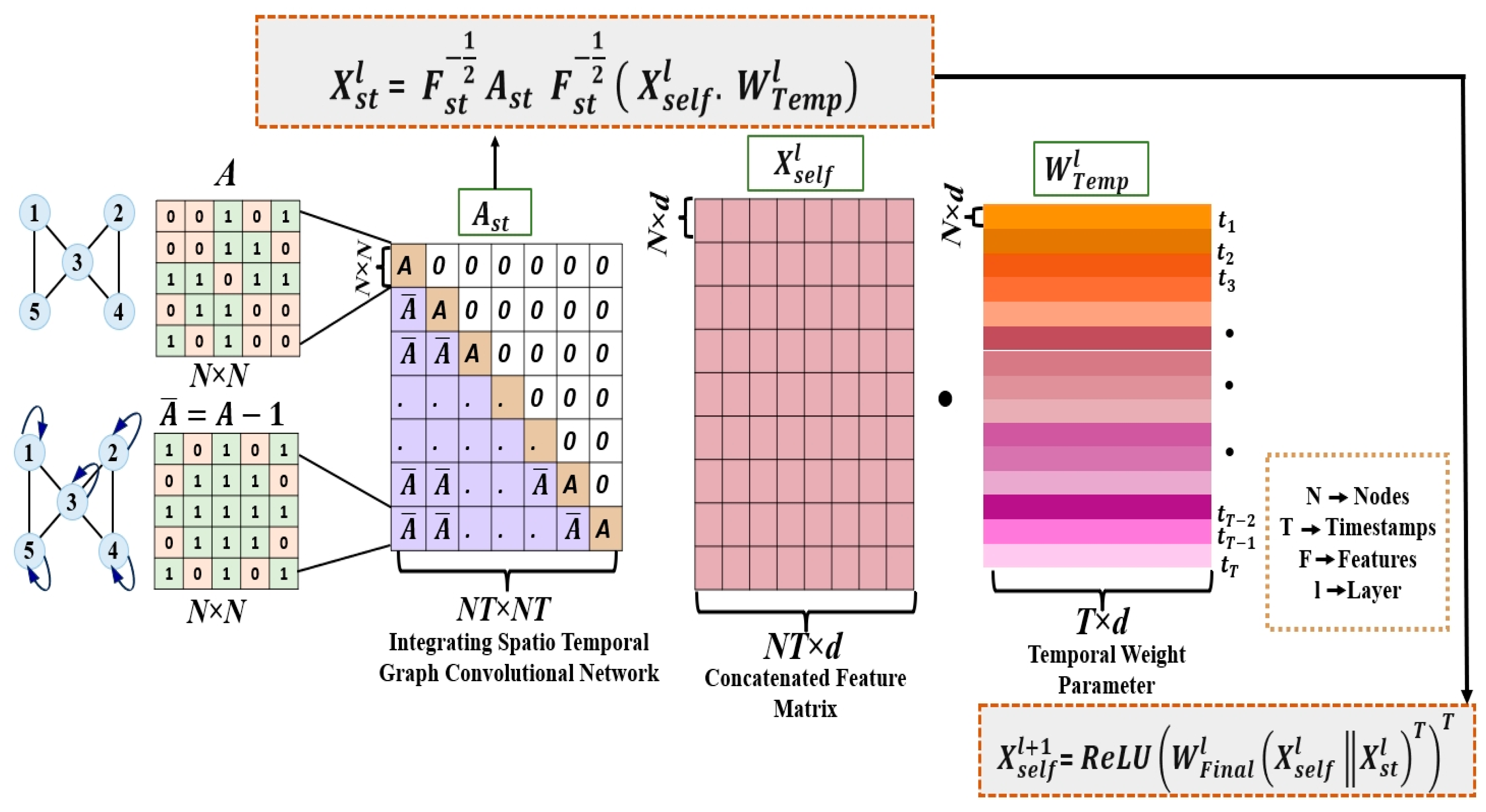
The graph convolutional network (GCN) is used to aggregate spatial information from neighboring nodes. Each node’s feature matrix $x_{s\left.e\right|f}^l$ at layer l is updated by considering the features of its neighbors, weighted by the adjacency matrix. The propagation rule for the spatial convolution at layer l is given by:

$$X_{Self}^{l+1}=\sigma \left(F_{st}^{-{\displaystyle \frac{1}{2}}}{A}_{st}{F}_{st}^{-{\displaystyle \frac{1}{2}}}{X}_{self}^l{W}_{spatial}^l\right)$$

(3)

where A_st is the adjacency matrix representing the spatial relationships between nodes. F_st is the degree matrix used for normalization. $X_{self}^l$ is the node feature matix at layer l, $W_{spatial}^l$ is a learnable weight matrix for the spatial transformation, and $\sigma$ is a non-linear activation function. This equation aggregates information from neighboring nodes in the graph, allowing each node to update its feature representation by incorporating the features of spatially adjacent nodes. Figure 2 presents the ISTGCN architecture Graph convolution is applied as self representation $X_{self}^l$, which is combined with the spatio-temporal aggregated vector $X_{ST}^l$ using weighted fusion. This result is represented as $X_{self}^{l+1}$, which serves as input for the next layer l + 1 or is passed into the regression task.

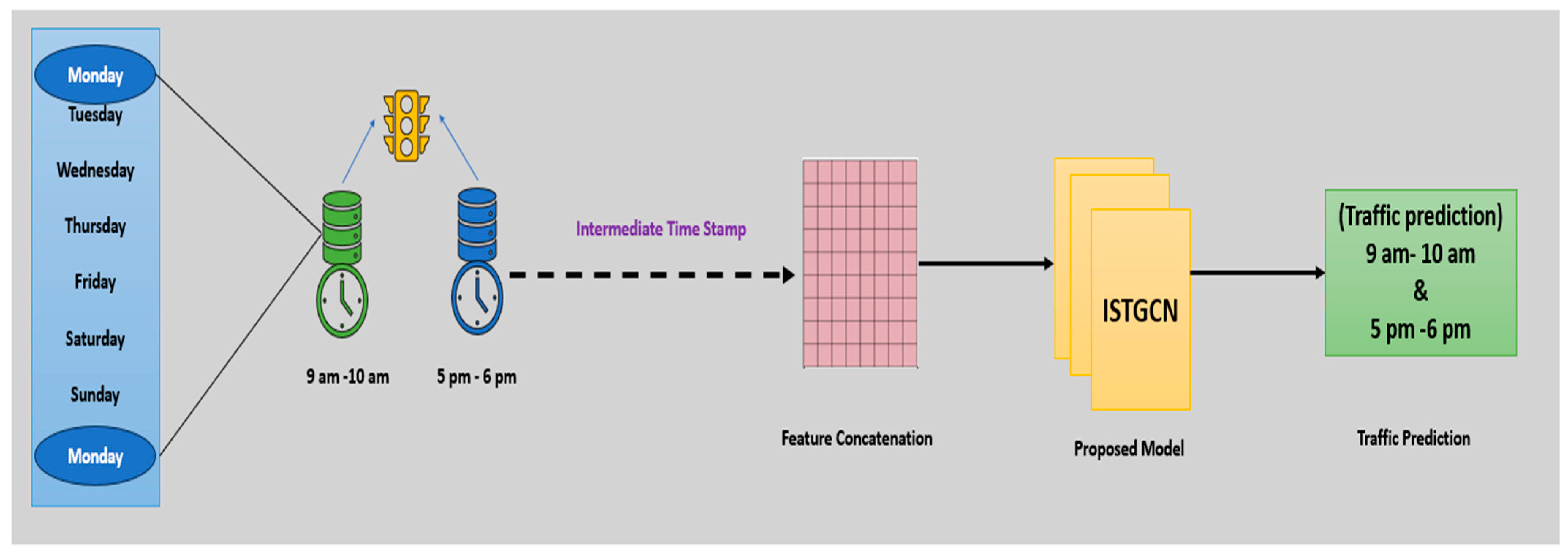
Figure 3, illustrates the process of traffic prediction using the ISTGCN model. Traffic data are collected across multiple days of the week (Monday to Sunday) for two specific time intervals each day: 9 AM to 10 AM and 5 PM to 6 PM, marked by green and blue icons. These data, including last week’s Monday traffic data, are passed through an intermediate step called “Intermediate Time Stamp”, where traffic information from different days and times is aggregated into a feature matrix. The feature matrix represents traffic speeds or conditions at various nodes in the network. This matrix is then fed into the ISTGCN model, which processes the spatio-temporal data using graph convolutional networks. The model uses these historical data to predict future traffic, for example, using last week’s Monday data to predict traffic for the next Monday. Finally, the model predicts traffic intensities specifically for the two peak time intervals, 9 AM to 10 AM and 5 PM to 6 PM.

4. Experimental Analysis

In this section, we provide a detailed overview of the datasets and the experimental setup, followed by a comprehensive analysis of the experiments.

4.1. Dataset Description

To validate the efficacy of our proposed model, we conducted experiments on three publicly available real-world traffic datasets: PeMSD7 and PeMSD8, which are collected by the Caltrans Performance Measurement System (PeMS) [9]. These datasets are widely recognized in traffic forecasting research and have been used for performance benchmarking in previous studies like STGCN [33], ASTGCN [34], and LSGCN [35]. We followed the data partitioning strategy used in LSGCN to divide the datasets into training and testing sets. A summary of the dataset statistics is provided in

Table 1. Road traffic dataset description.

Statistics	PeMSD7	PeMSD8
No. of nodes	220	170
No. of edges	832	295
Timestamp	12,672	17,856
Time interval	5 min	5 min
Daily range	00:00–24:00	00:00–24:00

.

• PeMSD7: This dataset consists of traffic speed data collected from 228 sensors in District 7 of California, covering weekdays from May to June 2012, with a 5 min time interval. We used the first month of data for training and the remainder for validation and testing.
• PeMSD8: This dataset contains traffic data from San Bernardino, recorded between July and August 2016, with 170 detectors across 8 roads, also at 5 min intervals. The initial fifty days are used for training, while the subsequent data serve for validation and testing.

4.2. Data Processing

In all three datasets, the data are recorded at regular intervals of 5 min, resulting in 288 timestamps per day. For the PeMSD7 dataset, the adjacency matrix of the traffic network is constructed using a threshold Gaussian kernel.

$$A_{ij}=\left\{\begin{array}{c}\mathit{exp}\left({\displaystyle \frac{-d_{ij}^2}{\delta }}, if i is not equal to j \left({\displaystyle \frac{-d_{ij}^2}{\delta }}\right) \ge \mathsf{ϵ}\right):\\ 0, otherwise\end{array}\right.$$

For PeMSD8, the adjacency matrix is similarly constructed as

$$A_{ij}=\left\{\begin{array}{c}\mathit{exp}\left({\displaystyle \frac{-d_{ij}^2}{\delta }}, if i and j are neighbors\right):\\ 0, otherwise\end{array}\right.$$

Here, $A_{ij}$ represents the edge weight between sensors i and j and d_ij is the physical distance between them. To control the sparsity and distribution of adjacency matrix A, the thresholds are $\delta$ = 0.1 and $\mathsf{ϵ}$ = 0.5.

This description explains how time stamps and their frequency are used in the model for traffic prediction. The time stamps have a frequency of 5 min, meaning there are 12 time stamps in one hour (since 60 min divided by 5 min gives 12). These time stamps overlap with the periods to provide contextual information about the traffic pattern at different times of the day. To capture periodic patterns, such as daily and weekly trends, a positional embedding is generated using a sinusoidal function, which helps represent the time-specific characteristics in the data. This is particularly useful for recognizing patterns that recur within the day or week. Additionally, each time step corresponds to 5 min, and for an hour, there would be 12 time steps. This hourly sampling helps calculate how many time steps fit into any given prediction window. The prediction interval, expressed in minutes, is calculated as (pred_len * 5), assuming each step represents 5 min. For example, if the prediction length is 6, the interval would be 30 min (6 * 5). The dataset assumes that each time stamp corresponds to a 5 min interval, meaning there are 288 time stamps in a 24 h period (for 24 h × 12 time stamps/hour = 288). For the morning traffic period from 9 AM to 10 AM, the corresponding time stamps would range from 108 to 120, as this period falls within the 288 time stamps representing the entire day. This structure is used to capture historical data over certain periods and predict future traffic conditions based on the defined intervals.

4.3. Result and Analysis

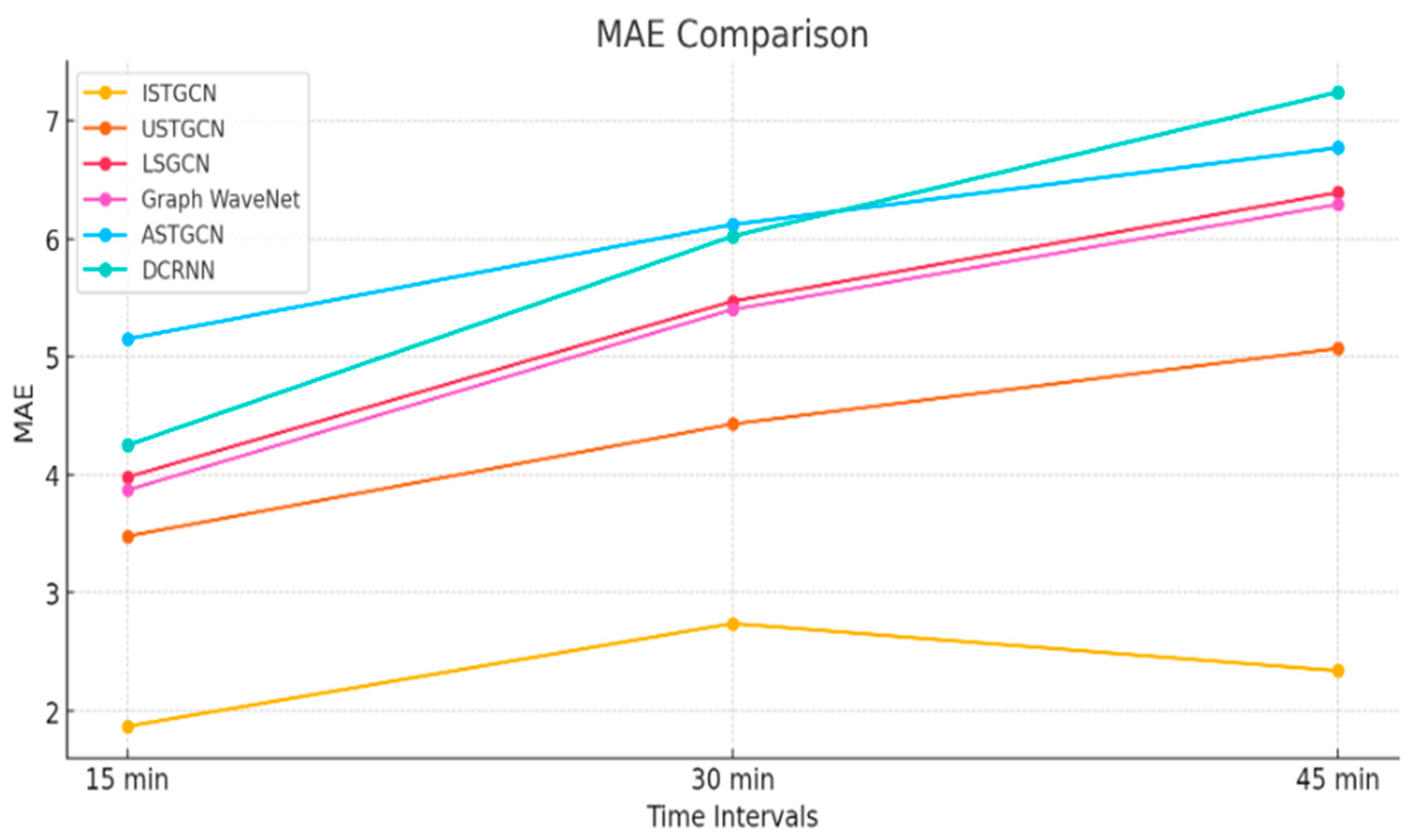
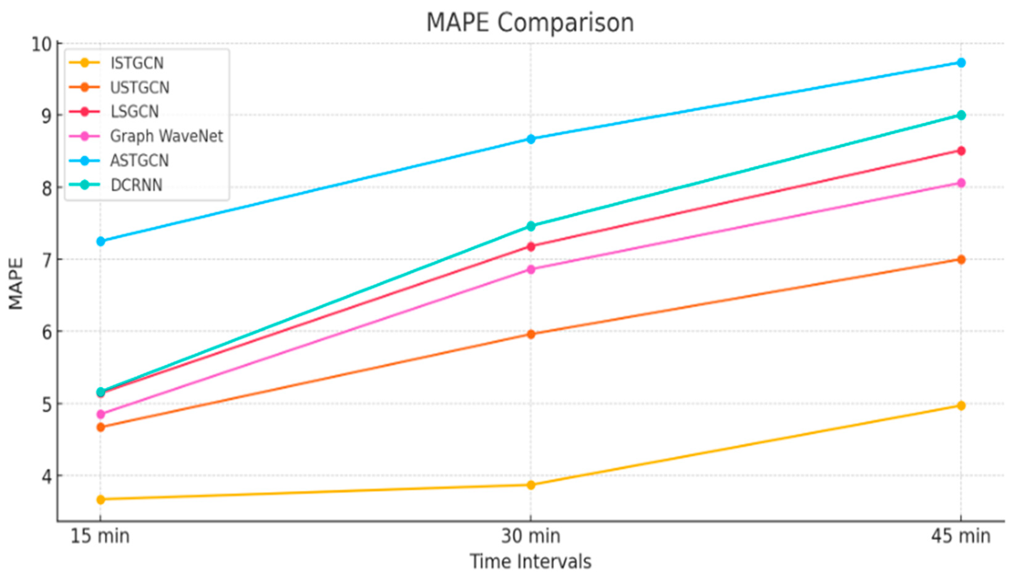
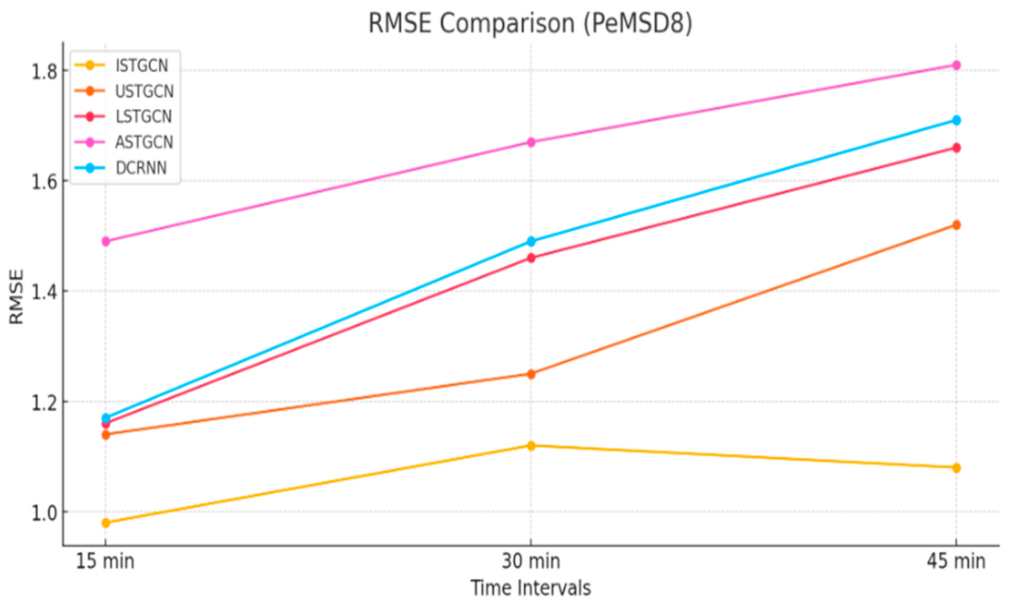
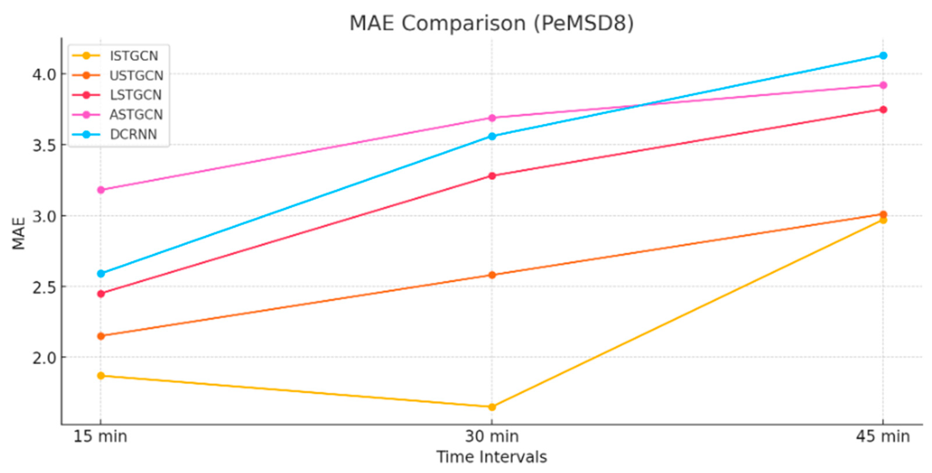
The results of our proposed ISTGCN model highlight its ability to outperform state-of-the-art traffic prediction models, including USTGCN [36], LSGCN [35], Graph WaveNet [37], ASTGCN [34], and DCRNN [38], across multiple time intervals (15, 30, 45 min). When evaluating key error metrics—root mean squared error (RMSE), mean absolute error (MAE), and mean absolute percentage error (MAPE)—our model consistently achieves lower values, signifying greater prediction accuracy and reliability. The ISTGCN model leverages an enhanced integration of spatio-temporal dependencies through graph convolutional networks, which allows it to capture complex traffic dynamics more effectively than existing models. Compared to USTGCN, which serves as a baseline for spatio-temporal graph convolutional networks, ISTGCN exhibits significantly lower RMSE and MAPE values, particularly for long-term forecasts (45 min). This improvement stems from ISTGCN’s ability to maintain a robust balance between spatial and temporal features without sacrificing prediction quality over time.

Similarly, ISTGCN demonstrates superior performance over LSGCN, a model that employs localized spatial-temporal convolution. Our model delivers a more refined understanding of the spatial dependencies between traffic sensors, resulting in lower MAE and RMSE values, especially in longer prediction intervals. In comparison with Graph WaveNet, which has been competitive in handling time-series data, ISTGCN excels in reducing both MAE and MAPE, providing more accurate short-term predictions (15 and 30 min) by better modeling spatial relations. In terms of accuracy, ISTGCN also surpasses ASTGCN, which uses an attention mechanism for spatio-temporal data. The lower RMSE and MAE of ISTGCN suggest that its architecture avoids potential overfitting and provides more consistent performance across various time frames. Finally, compared to DCRNN, an earlier recurrent neural network-based approach, ISTGCN significantly reduces errors in all metrics, highlighting the limitations of recurrent models in capturing long-range dependencies and the advantages of convolutional approaches in this domain. Overall, the ISTGCN model demonstrates its superiority through lower error values across all metrics, highlighting its robustness in handling complex traffic data. The significant reduction in RMSE, MAE, and MAPE confirms that ISTGCN offers more precise traffic predictions, effectively modeling both the spatial and temporal aspects of the data, thus making it the most reliable model for traffic forecasting compared to its peers.

Table 2. Comparison analysis with another model.

Dataset	Model	15 min			30 min			45 min
		RMSE	MAE	MAPE	RMSE	MAE	MAPE	RMSE	MAE	MAPE
PeMSD7	ISTGCN [Proposed]	1.03	1.87	3.67	1.60	2.74	3.87	2.09	2.34	4.97
	USTGCN [36]	2.01	3.48	4.67	2.46	4.43	5.96	2.89	5.07	7.00
	LSGCN [35]	2.22	3.98	5.14	2.96	5.47	7.18	3.43	6.39	8.51
	Graph WaveNet [37]	2.17	3.87	4.85	2.90	5.40	6.86	3.23	6.29	8.06
	ASTGCN [34]	2.85	5.15	7.25	3.35	6.12	8.67	3.70	6.77	9.73
	DCRNN [38]	2.22	4.25	5.16	3.04	6.02	7.46	3.64	7.24	9.00
PeMSD8	ISTGCN [Proposed]	0.98	1.87	1.06	1.12	1.65	1.45	1.08	2.97	1.98
	USTCGN [36]	1.14	2.15	2.07	1.25	2.58	2.35	1.52	3.01	2.88
	LSTCGN [35]	1.16	2.45	2.24	1.46	3.28	3.02	1.66	3.75	3.51
	ASTGCN [34]	1.49	3.18	3.16	1.67	3.69	3.59	1.81	3.92	3.98
	DCRNN [38]	1.17	2.59	2.32	1.49	3.56	3.21	1.71	4.13	3.83

evaluates the performance of various spatio-temporal graph learning models—ISTGCN, USTGCN, LSGCN, Graph WaveNet, ASTGCN, and DCRNN—on traffic prediction tasks using two datasets, PeMSD7 and PeMSD8. The models predict traffic at three different future time intervals (15, 30, and 45 min) and are assessed using three widely recognized error metrics: root mean squared error (RMSE), mean absolute error (MAE), and mean absolute percentage error (MAPE). These metrics help measure how accurately the models predict traffic conditions, with lower values indicating better performance.

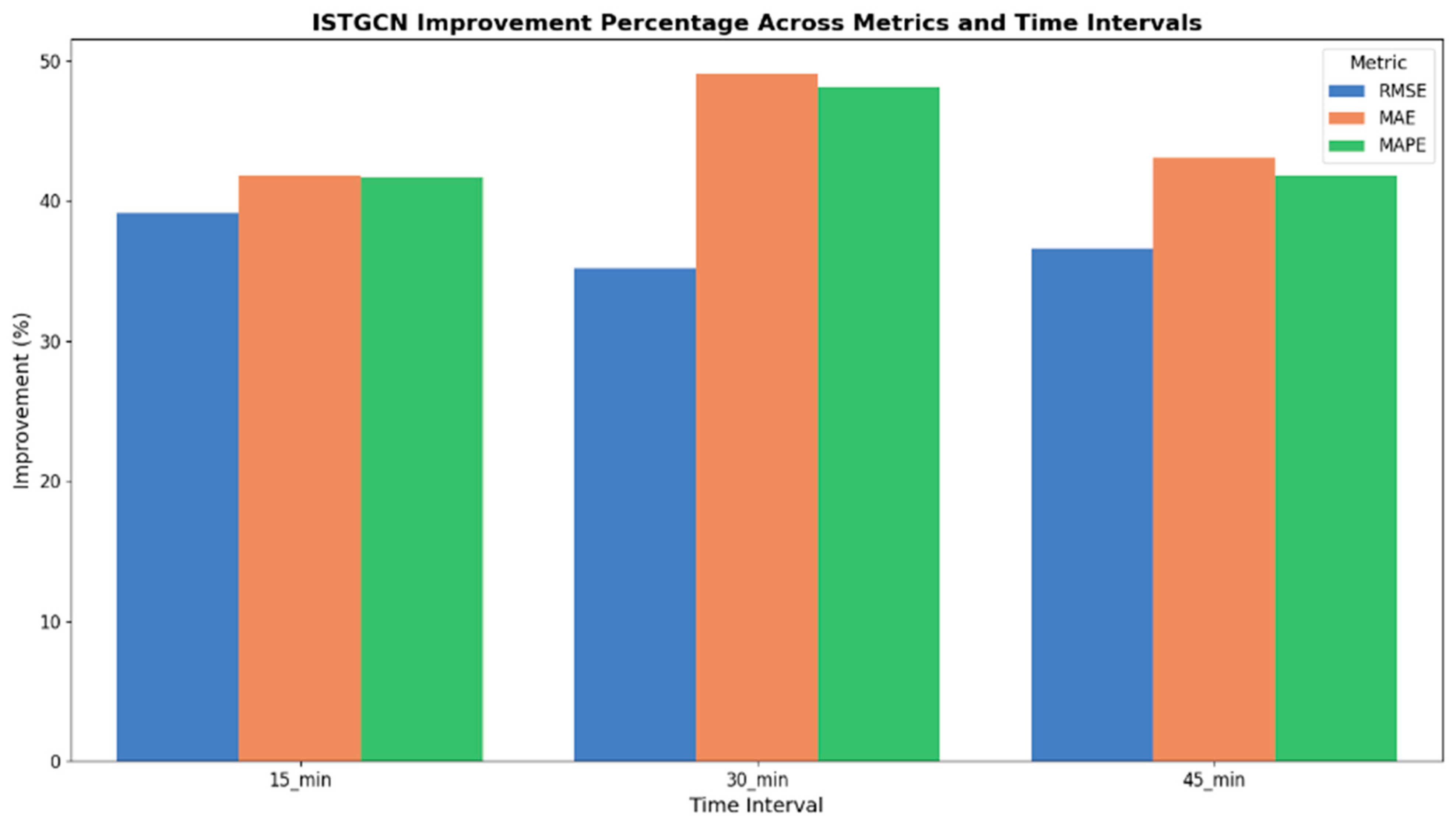
The Figure 4 bar chart illustrates the percentage improvement of the ISTGCN (proposed) model over other models (USTGCN, LSGCN, Graph WaveNet, ASTGCN, and DCRNN) across three evaluation metrics—RMSE, MAE, and MAPE—over prediction intervals of 15, 30, and 45 min. ISTGCN consistently outperforms its competitors, demonstrating substantial improvements in reducing RMSE and MAE, which measure numerical accuracy and error magnitude, respectively. MAPE improvements, though slightly lower, highlight ISTGCN’s reliability in minimizing percentage errors. The highest gains are observed for the 15 min interval, particularly for RMSE and MAE, with the improvements slightly diminishing for longer horizons, as expected in time-series predictions. Overall, the ISTGCN proves to be robust and effective, delivering consistently better predictive performance across both short and moderately extended time intervals, making it a strong choice for real-world applications requiring accurate and reliable forecasts.

$$Improvemt \%={\displaystyle \frac{\left(Performance of Other model-Performance of ISTGCN\right)\times 100}{Performance of other model}}$$

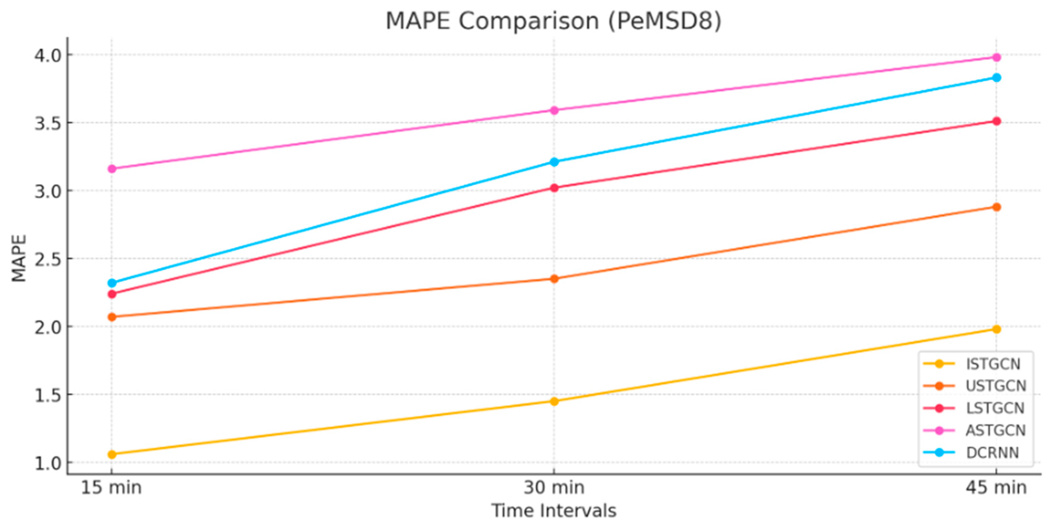
The graph is based on a mathematical formula that calculates the percentage improvement of the ISTGCN (proposed) model compared to other models. The formula measures the relative reduction in error achieved by ISTGCN for metrics such as RMSE, MAE, and MAPE. Specifically, the improvement percentage is determined by subtracting ISTGCN’s error value from the error value of another model, dividing this difference by the other model’s error value, and then multiplying the result by 100 to express it as a percentage. This calculation is performed for each metric across three time intervals (15, 30, and 45 min) and for both datasets (PeMSD7 and PeMSD8). The resulting percentage improvements are then plotted in the graph to highlight ISTGCN’s consistent superiority over its counterparts in minimizing errors, particularly for shorter time intervals and across all metrics (Figure 5, Figure 6, Figure 7, Figure 8, Figure 9 and Figure 10).

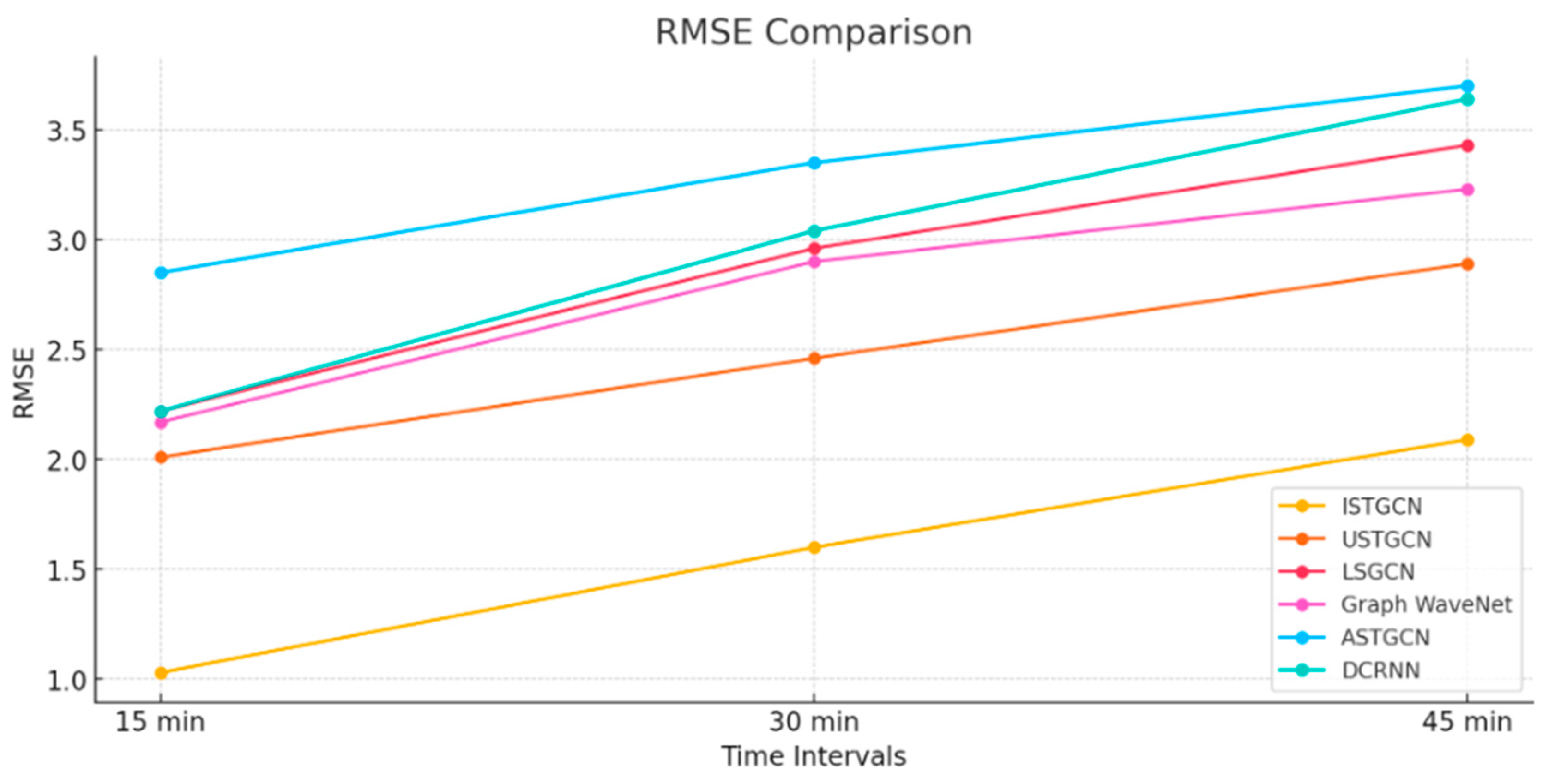
ISTGCN stands out significantly by achieving the lowest error rates across all metrics and time intervals, making it the best-performing model. For example, on the PeMSD7 dataset, ISTGCN records an RMSE of 1.03 at 15 min, which is considerably lower than other models like USTGCN and LSGCN, which have RMSE values above 2. Similarly, on the PeMSD8 dataset, ISTGCN maintains its superior performance with an RMSE of 0.98 at 15 min. This indicates that ISTGCN is particularly effective at making accurate short-term and medium-term traffic predictions.

In contrast, models like ASTGCN and DCRNN show much higher error rates, especially for longer forecasting horizons. For instance, ASTGCN’s RMSE increases to 3.70 at 45 min on PeMSD7, highlighting its struggle with long-term predictions. Additionally, models such as USTGCN, LSGCN, and Graph WaveNet also show declining performance as the prediction interval increases, with error metrics rising steadily from 15 to 45 min. The overall trend shows that all models tend to perform less effectively compared to ISTGCN as the forecasting horizon extends, but ISTGCN consistently outperforms all other deep learning models, maintaining lower error rates across all time intervals and datasets. This highlights ISTGCN’s robustness in traffic prediction, proving its ability to make more accurate and reliable forecasts compared to the rest of the deep learning models.

5. Conclusions

In this paper, we introduced ISTGCN, a novel spatio-temporal graph convolution network designed for traffic prediction, which consistently outperforms several state-of-the-art models. Our experimental results across multiple real-world traffic datasets demonstrate that ISTGCN achieves significantly lower error values across key metrics—RMSE, MAE, and MAPE—compared to models such as USTGCN, LSGCN, Graph WaveNet, ASTGCN, and DCRNN. Specifically, our model demonstrates an overall reduction of 37.80% in RMSE, 46.75% in MAE, and 28.49% in MAPE compared to the USTGCN model. These reductions highlight the improved accuracy and reliability of our proposed model in both short- and long-term traffic forecasting. ISTGCN leverages a more effective integration of spatio-temporal features, enabling it to better capture complex traffic patterns, especially over longer prediction intervals (15, 30, and 45 min). This results in enhanced predictive performance and reduced errors, particularly in long-term forecasts. These findings demonstrate the robustness of ISTGCN in modeling real-time traffic data, making it a more accurate and efficient solution for intelligent transportation systems.

References

1. Jiang, W.; Zhang, L. Geospatial data to images: A deep-learning framework for traffic forecasting. Tsinghua Sci. Technol. 2018, 24, 52–64. [Google Scholar] [CrossRef]
2. Singh, V.; Sahana, S.K.; Bhattacharjee, V. Graph convolutional neural networks for traffic forecasting and prediction: A review. AIP Conf. Proc. 2024, 3164, 040003. [Google Scholar]
3. Liu, L.; Chen, J.; Wu, H.; Zhen, J.; Li, G.; Lin, L. Physical-virtual collaboration modelling for intra-and inter-station metro ridership prediction. IEEE Trans. Intell. Transp. Syst. 2020, 23, 3377–3391. [Google Scholar] [CrossRef]
4. Wu, Z.; Pan, S.; Long, G.; Jiang, J.; Chang, X.; Zhang, C. Connecting the dots: Multivariate time series forecasting with graph neural networks. In Proceedings of the 26th ACM SIGKDD International Conference on Knowledge Discovery & Data Mining, Virtual Event, CA, USA, 6–10 July 2020; pp. 753–763. [Google Scholar]
5. Sharma, A.; Sharma, A.; Nikashina, P.; Gavrilenko, V.; Tselykh, A.; Bozhenyuk, A.; Masud, M.; Meshref, H.A. A graph neural network (GNN)-based approach for real-time traffic speed estimation in sustainable smart cities. Sustainability 2023, 15, 11893. [Google Scholar] [CrossRef]
6. Alahi ME, E.; Sukkuea, A.; Tina, F.W.; Nag, A.; Kurdthongmee, W.; Suwannarat, K.; Mukhopadhyay, S.C. Integration of IoT-Enabled Technologies and Artificial Intelligence (AI) for Smart City Scenario: Recent Advancements and Future Trends. Sensors 2023, 23, 5206. [Google Scholar] [CrossRef]
7. Gohar, M.; Muzammal, M.; Rahman, A.U. SMART TSS: Defining transportation system behavior using big data analytics in smart cities. Sustain. Cities Soc. 2018, 41, 114–119. [Google Scholar] [CrossRef]
8. Ahmed, M.S.; Cook, A.R. Analysis of freeway traffic time-series data by using Box-Jenkins techniques. (No. 722) 1979. Available online: https://trid.trb.org/View/148123 (accessed on 21 October 2024).
9. Chen, C.; Petty, K.; Skabardonis, A.; Varaiya, P.; Jia, Z. Freeway performance measurement system: Mining loop detector data. Transp. Res. Rec. 2001, 1748, 96–102. [Google Scholar] [CrossRef]
10. Abadi, A.; Rajabioun, T.; Ioannou, P.A. Traffic flow prediction for road transportation networks with limited traffic data. IEEE Trans. Intell. Transp. Syst. 2014, 16, 653–662. [Google Scholar] [CrossRef]
11. Yang, X.; Tang, L.; Stewart, K.; Dong, Z.; Zhang, X.; Li, Q. Automatic change detection in lane-level road networks using GPS trajectories. Int. J. Geogr. Inf. Sci. 2018, 32, 601–621. [Google Scholar] [CrossRef]
12. Boukerche, A.; Wang, J. Machine learning-based traffic prediction models for intelligent transportation systems. Comput. Netw. 2020, 181, 107530. [Google Scholar] [CrossRef]
13. Manley, E. Estimating urban traffic patterns through probabilistic interconnectivity of road network junctions. PLoS ONE 2015, 10, e0127095. [Google Scholar] [CrossRef] [PubMed]
14. Li, H.; Lu, H.; Jensen, C.S.; Tang, B.; Cheema, M.A. Spatial data quality in the Internet of Things: Management, exploitation, and prospects. ACM Comput. Surv. (CSUR) 2022, 55, 1–41. [Google Scholar] [CrossRef]
15. Guo, Y.; Zhang, Y.; Boulaksil, Y.; Tian, N. Multi-dimensional spatiotemporal demand forecasting and service vehicle dispatching for online car-hailing platforms. Int. J. Prod. Res. 2022, 60, 1832–1853. [Google Scholar] [CrossRef]
16. Krüger, N.A. Estimating traffic demand risk–a multiscale analysis. Transp. Res. Part A Policy Pract. 2012, 46, 1741–1751. [Google Scholar] [CrossRef]
17. Yu, B.; Li, M.; Zhang, J.; Zhu, Z. 3D graph convolutional networks with temporal graphs: A spatial information free framework for traffic forecasting. arXiv 2019, arXiv:1903.00919. [Google Scholar]
18. Feng, A.; Tassiulas, L. Adaptive Graph Spatial-Temporal Transformer Network for Traffic Forecasting. In Proceedings of the 31st ACM International Conference on Information & Knowledge Management, Atlanta, GA, USA, 17–21 October 2022; pp. 3933–3937. [Google Scholar]
19. Zhang, M.; Li, Y.; Sun, F.; Guo, D.; Hui, P. Adaptive spatio-temporal convolutional network for traffic prediction. In Proceedings of the 2021 IEEE International Conference on Data Mining (ICDM), Auckland, New Zealand, 7–10 December 2021; IEEE: Piscataway, NJ, USA, 2021; pp. 1475–1480. [Google Scholar]
20. Wei, L.; Yu, Z.; Jin, Z.; Xie, L.; Huang, J.; Cai, D.; He, X.; Hua, X.-S. Dual graph for traffic forecasting. IEEE Access 2019. [Google Scholar] [CrossRef]
21. Waikhom, L.; Patgiri, R.; Singh, L.D. Dynamic temporal position observant graph neural network for traffic forecasting. Appl. Intell. 2023, 53, 23166–23178. [Google Scholar] [CrossRef]
22. Li, S.; Jin, X.; Xuan, Y.; Zhou, X.; Chen, W.; Wang, Y.X.; Yan, X. Enhancing the locality and breaking the memory bottleneck of transformer on time series forecasting. In Proceedings of the 33rd International Conference on Neural Information Processing Systems, Vancouver, BC, Canada, 8–14 December 2019; Advances in neural information processing systems. Volume 32. [Google Scholar]
23. Zhang, C.; Zhang, S.; James, J.Q.; Yu, S. FASTGNN: A topological information protected federated learning approach for traffic speed forecasting. IEEE Trans. Ind. Inform. 2021, 17, 8464–8474. [Google Scholar] [CrossRef]
24. Ge, L.; Li, S.; Wang, Y.; Chang, F.; Wu, K. Global spatial-temporal graph convolutional network for urban traffic speed prediction. Appl. Sci. 2020, 10, 1509. [Google Scholar] [CrossRef]
25. Jiang, W.; Luo, J. Graph neural network for traffic forecasting: A survey. Expert Syst. Appl. 2022, 207, 117921. [Google Scholar] [CrossRef]
26. Zhang, C.; Zhang, S.; Yu, S.; James, J.Q. Graph-based traffic forecasting via communication-efficient federated learning. In Proceedings of the 2022 IEEE Wireless Communications and Networking Conference (WCNC), Austin, TX, USA, 10–13 April 2022; IEEE: Piscataway, NJ, USA, 2022; pp. 2041–2046. [Google Scholar]
27. Ambrose, S.A.; Wankel, L.A. Higher Education’s Road to Relevance: Navigating Complexity; John Wiley & Sons: Hoboken, NJ, USA, 2020. [Google Scholar]
28. Lemonde, C.; Arsenio, E.; Henriques, R. Integrative analysis of multimodal traffic data: Addressing open challenges using big data analytics in the city of Lisbon. Eur. Transp. Res. Rev. 2021, 13, 64. [Google Scholar] [CrossRef]
29. Sayed, S.A.; Abdel-Hamid, Y.; Hefny, H.A. Artificial intelligence-based traffic flow prediction: A comprehensive review. J. Electr. Syst. Inf. Technol. 2023, 10, 13. [Google Scholar] [CrossRef]
30. Nasr Azadani, M. Driving Behavior Analysis and Prediction for Safe Autonomous Vehicles. Doctoral Dissertation, Université d’Ottawa/University of Ottawa, Ottawa, ON, USA, 2024. [Google Scholar]
31. Luo, Q.; He, S.; Han, X.; Wang, Y.; Li, H. LSTTN: A Long-Short Term Transformer-based Spatiotemporal Neural Network for Traffic Flow Forecasting. Knowl.-Based Syst. 2024, 293, 111637. [Google Scholar] [CrossRef]
32. He, S.; Luo, Q.; Fu, X.; Zhao, L.; Du, R.; Li, H. CAT: A Causally Graph Attention Network for Trimming Heterophilic Graph. Inf. Sci. 2024, 667, 120916. [Google Scholar] [CrossRef]
33. Yu, B.; Yin, H.; Zhu, Z. Spatio-temporal graph convolutional networks: A deep learning framework for traffic forecasting. In Proceedings of the 27th International Joint Conference on Artificial Intelligence, Stockholm, Sweden, 13–19 July 2018. [Google Scholar]
34. Guo, S.; Lin, Y.; Feng, N.; Song, C.; Wan, H. Attention based spatialtemporal graph convolutional networks for traffic flow forecasting. In Proceedings of the AAAI’19: AAAI Conference on Artificial Intelligence, Honolulu, HI, USA, 27 January–1 February 2019. [Google Scholar]
35. Huang, R.; Huang, C.; Liu, Y.; Dai, G.; Kong, W. Lsgcn: Long shortterm traffic prediction with graph convolutional networks. In Proceedings of the Twenty-Ninth International Joint Conference on Artificial Intelligence, Yokohama, Japan, 7–15 January 2020. [Google Scholar]
36. Roy, A.; Roy, K.K.; Ali, A.A.; Amin, M.A.; Rahman, A.M. Unified spatio-temporal modeling for traffic forecasting using graph neural network. In Proceedings of the 2021 International Joint Conference on Neural Networks (IJCNN), Shenzhen, China, 18–22 July 2021; IEEE: Piscataway, NJ, USA, 2021; pp. 1–8. [Google Scholar]
37. Wu, Z.; Pan, S.; Long, G.; Jiang, J.; Zhang, C. Graph wavenet for deep spatial-temporal graph modeling. In Proceedings of the 28th International Joint Conference on Artificial Intelligence, Macao, China, 10–16 August 2019. [Google Scholar]
38. Li, Y.; Yu, R.; Shahabi, C.; Liu, Y. Diffusion convolutional recurrent neural network: Data-driven traffic forecasting. arXiv 2017, arXiv:1707.01926. [Google Scholar]
Figure 1. Graph-structured traffic data, denoted as vt, represents the current traffic status at time step t in matrix format.
Applsci 14 11477 g001
Figure 2. Integrated spatio-temporal graph convolutional network architecture.
Applsci 14 11477 g002
Figure 3. Traffic prediction using ISTGCN.
Applsci 14 11477 g003
Figure 4. Improvement percentage of proposed model ISTGCN.
Applsci 14 11477 g004
Figure 5. PeMSD7 dataset with RMSE comparison with other models.
Applsci 14 11477 g005
Figure 6. PeMSD7 dataset with MAE comparison with other models.
Applsci 14 11477 g006
Figure 7. PeMSD7 dataset with MAPE comparison with other models.
Applsci 14 11477 g007
Figure 8. PeMSD8 dataset with RMSE comparison with other models.
Applsci 14 11477 g008
Figure 9. PeMSD8 dataset with MAE comparison with other models.
Applsci 14 11477 g009
Figure 10. PeMSD8 dataset with MAPE comparison with other models.
Applsci 14 11477 g010