Abstract
One of the key elements in real estate appraisal of residential buildings is the usable area. To determine the monetary value of real estate, appraisers in Poland often rely on transaction data registered in the Real Estate Price Register (REPR). However, the REPR may contain meaningful gaps, particularly on information concerning usable areas. This may lead to difficulties in finding suitable comparative properties, resulting in mispricing of the property. To address this problem, we used linear and nonlinear models to estimate the usable area of buildings with multi-pitched roofs. Utilizing widely available data from the Topographic Objects Database (BDOT10k) based on LiDAR technology, we have shown that three parameters (building’s covered area, building’s height, and optionally the number of storeys) are sufficient for a reliable estimate of the usable area of a building. The best linear model, using design data from architectural offices, achieved a fit of 95%, while the best model based on real data of existing buildings in the city of Koszalin, Poland achieved 92% fit. The best nonlinear model achieved slightly better results than the linear model in the case of design data (better fit by approximately 0.2%). In the case of existing buildings in Koszalin, the best fit was at 93%. The proposed method may help property appraisers determine a more accurate estimation of the usable area of comparative buildings in the absence of this information in the REPR.
1. Introduction
A comparative approach is the most reliable and common real estate appraisal method [1,2]. The appraiser compares the examined property with similar buildings recently sold on the local market to evaluate the property’s price. One of the main parameters for such comparisons, especially in the case of residential properties, is their usable area [3,4]. To search for comparative transactions, Polish appraisers most often use the public Real Estate Price Register (REPR, in Polish: Rejestr Cen Nieruchomości). The REPR was introduced in Poland in 2001 initially under name “Register of Prices and Values of Real Estate”. At that time, all legal regulations concerning the database were regulated by the Regulation of the Minister of Regional Development and Construction of 29 March 2001 “On the land and building register” [5]. In 2021, in connection with the introduction of changes and a new legal act, a new database, the Real Estate Price Register (REPR), was created. The REPR is a public register maintained by local authorities (e.g., mayor’s offices) and operating in a country-wide ICT system. It includes data on real estate prices specified in notarial deeds. Detailed regulations regarding the REPR are specified in the Regulation of the Minister of Development, Labour and Technology of 27 July 2021 on the land and building register. The REPR is also part of the Cadastre [6,7,8,9,10,11,12,13]. Unfortunately, several studies revealed deficiencies in the REPR, especially concerning data on the usable areas of residential buildings [14,15,16]. For example, a study involving 800 residential buildings covered in the REPR in the counties of Koszalin and Kolobrzeg revealed that information on usable area was available only in about 40% of properties [16]. This limited data availability can significantly hinder the search for comparable transactions. Particularly in small local markets, with only few similar property transactions, real estate appraisal using the comparative method is therefore highly questionable.
Calculating a building’s usable area is also a complex issue. Several publications [17,18,19,20,21] show that the standards named in the Polish legislation that specify the rules for measuring and defining usable area are rather complicated. Until 1999, the usable area was commonly calculated according to the PN-B-02365:1970 standard [22]. Calculating the usable area according to this standard included only spaces that can be used for their intended purpose, including living rooms, kitchens, and bathrooms. However, when measuring the usable area, it is also important to consider the slopes of the roof in properties with an attic. In this case, different regulations apply depending on the height of the walls. Another common standard was PN-ISO 9836:1997 [23], which considered spaces such as basements, boiler rooms, garages, or other utility spaces that were not used directly for living not applicable to usable area. In the years 1999–2012, both standards were in force. After 2012, the PN-ISO 9836:1997 standard became mandatory for newly built properties. Over time, additional rules were also introduced which significantly affected the method of calculating the usable area [24]. Furthermore, the Polish Committee for Standardization withdrew PN-B-02365:1970 and PN-ISO 9836:1997, and since 2015, the recommended standard is PN-ISO 9836:2015-12 [25]. This standard introduced updated definitions and measurement procedures consistent with international standards. This standard specifies the method of calculating the usable area on different floors, including sloping ceilings and attic space. The standard places particular emphasis on the precision of measurements in residential and commercial buildings and eliminates potential discrepancies in the interpretation of previous guidelines. The regulation of usable areas introduced changes in the way indoor spaces are measured and classified. The updated rules also consider changing construction technologies and the way real estate is used. The standard has been adapted to European standards, which makes it easier to compare properties within European Union markets. An additional difficulty for real estate appraisers in Poland using the REPR is the lack of information regarding the standards the usable area of the building was calculated by. A lack of full compliance between older standards and new regulations can lead to differences in the interpretation and results of property appraisal. The errors can range from a few to several percent, depending on the architecture of the building and the standard used. A detailed description of the norms and differences between standards can be found in the literature [26,27].
In this article, estimates of the usable area of detached residential buildings with multi-pitched roofs were conducted in accordance with the PN-ISO 9836:2015-12 standard. The PN-ISO 9836:2015-12 standard introduced new rules for calculating the usable area (especially in buildings with multi-pitched roofs) considering the slope of the roofs. According to these regulations, 100% of the area with a height > 2.2 m is included in the usable area; 50% of the area with a height between 1.4 and 2.2 m and areas < 1.4 m are excluded. An important consequence of this regulation is also the complete omission of partition walls, in contrast to the previous standards.
There is another publicly available source of data, the Database of Topographic Objects (hereafter referred to as BDOT10k) [28] that supports estimating the usable area of buildings. BDOT10k is a spatial database containing information about the topography of Poland. It collects detailed data on various landscape features, such as buildings, roads, rivers, forests, and railways, along with their descriptive attributes and location. The descriptions of the buildings in the database include features such as height, width, length, and perimeter. The main applications of BDOT10k are in spatial planning, environmental protection, real estate management, and technical infrastructure management. Users represent both the public administration and the private sector. This database provides accurate, unified data that is extremely useful for various types of spatial analysis, including building surface modelling and other geoinformation analysis. The information contained in BDOT10k comes from several sources, including airborne Light Detection and Ranging (LiDAR) scanning. Airborne LiDAR scanning is a remote sensing technique used to obtain precise information about the Earth’s surface, terrain objects, and more. LiDAR scanning involves the emission of laser pulses from a device mounted on an aircraft or drone, which bounce off the surface of the earth, buildings, trees, and other objects and then return to the sensor. Based on the return time of the pulses and the measured angle, the height and structure of the objects can be determined with high precision. In Poland, LiDAR data are provided by the Information System of the National Guard Program against Extraordinary Threats [29,30]. LiDAR scanning was carried out in Poland at two levels of detail (LoD): LoD1 and LoD2. The LoD1 level contains a square grid of measurement points with a density of 4 points/m2, omits the geometry of the roof and contains only building blocks. The LoD2 level is characterized by a rectangular grid of measurement points, with a grid density of 12 points/m2, containing roof structures and simple additional building textures, such as extensions or garages. Most of the LiDAR surface data in Poland shows the accuracy of LoD2, but the residential buildings analyzed in this article and located in Koszalin show the accuracy of LoD1, therefore they cannot be used to estimate the height of a building. The BDOT10k database is available in the Geoportal database managed by the Head Office of Geodesy and Cartography. Information for the city of Koszalin can been downloaded from the Geoportal in the CityGML 2.0 standard [31]. The information was accessed using QGIS Desktop v. 3.28.2. Google Street View was used when the REPR lacked information about the number of floors. Additionally, the data in the article come from notifications on the completion of the construction of residential buildings in Koszalin, sent to the District Inspector of Building Supervision in Koszalin. Such documents and permit applications are required to start using the buildings.
Using data from BDOT10k to estimate usable area has the potential to solve several problems of Polish appraisers. We propose the use of mathematical modelling to estimate the usable area of residential buildings with multi-pitched roofs based on topographic data. Although mathematical modelling is widely used in real estate valuation [32,33,34], it is rarely used to estimate other parameters of buildings other than value. Dawid et al. [26] demonstrated that the usable area of single-family houses with flat roofs can be precisely estimated using topographic data, neural networks, and regression analysis. Their study on 96 building designs from architectural offices and 29 existing buildings in Koszalin showed a high accuracy of estimating the usable area. The best neural network model, which was trained on building designs from design offices, was tested on real buildings in Koszalin. The estimation error was <9%, which can be considered a fairly good result. In a follow-up article [35] for residential buildings with a pitched roof based on data from architectural offices, it was shown that both linear regression and the neural network performed best when the input parameters were the building area, building height, number of floors, and knee wall height. The estimation error was 5% in the case of linear regression and 3% in the case of the neural network. For buildings built in different architectural styles between 2020 and 2022 in Koszalin that deviated significantly from the set from design offices, the accuracy of the best neural network estimate dropped to 15%.
Similarly to Dawid et al. [26,35], this article used two different datasets, namely architectural designs and existing buildings. The first justification is the fact that the designs from architectural offices contain full, detailed documentation of the building, in a known standard, which is not the case of existing buildings. Furthermore, a detailed description of the interior of the building and the structural solutions affecting the value of the usable area are known. Secondly, the existing data may contain measurement errors, which affects test quality. As the quality of linear and nonlinear models depends on the data quality, the use of precise architectural designs is a significant advantage. We have expanded our research to include residential buildings with multi-pitched roofs, which pose an additional challenge in estimating the usable area, due to the presence of slopes affecting the area of the top floor.
Multi-pitched roofs are roofs that have more than two sloping planes that connect at different angles [36]. Multi-pitched roofs are used primarily for their functionality, aesthetics, and durability. They offer several advantages compared with single-pitch or gable roofs. The slopes effectively drain rainwater and snow, which reduces the risk of leaking and structural damage. Due to their complex structure, multi-pitched roofs are more likely to withstand strong winds and other extreme weather conditions. Their shape dissipates wind forces, which increases the stability of the building. The slopes allow the space under the roof to be used more efficiently, which allows for arrangement of additional rooms (e.g., attics). Multi-pitched roofs have a more complex form, which affects the attractiveness of the building. They are often used in villa-type designs and modern residences, where aesthetics play an important role. Furthermore, the larger roof area facilitates the design of adequate ventilation, which improves living comfort and affects structure durability. Disadvantages of multi-pitched roofs include a fairly complicated structure, which entails a higher price than flat or gable roofs. There are several types of multi-pitched roofs, such as hipped, tented, mansard, monitor, and many others. In this article, the hip and multi-slope roofs were primarily considered. The hip roof has four bleeds, two in the shape of a triangle and two in the shape of a trapezoid. It is popular in single-family homes, providing even greater water drainage and aesthetic appearance. A multi-slope roof has many planes with different angles of inclination, connecting in different places. It is often used in buildings with a complex plan, such as houses with an extensive body.
An important parameter of a residential building with a multi-pitched roof is the height of the knee wall. This is described in more detail in [35], which analyses the parameters of the gable roof. The knee wall has a significant impact on the size of the usable area of the building, especially in the case of buildings with a usable attic. A higher knee wall makes more of the attic accessible and functional, as it increases the height of the side walls under the roof. With a higher knee wall, part of the space at the slanted ceilings, which would normally be too low for comfortable use, can be used as a full-fledged living space. As the height of the knee wall increases, the usable area of the building increases. With a low knee wall, the usable space is limited, which makes it difficult to arrange the interior, especially near the walls. A higher knee wall also provides more adaptability (e.g., better air circulation and furniture can be placed along the walls). Increasing the height of the knee wall also affects the external appearance of the building, which can be important from the perspective of aesthetics and architectural adaptation to the surroundings. Higher walls can make the building more massive, which should be considered when designing a multi-pitched roof. On the other hand, increasing the height of the knee wall is associated with higher construction costs, as this requires use of more materials and more complex construction solutions.
2. Materials and Methods
Reliable and complete data are necessary to estimate acceptable functional, linear, and nonlinear models or to effectively train machine learning models to estimate the usable area of buildings. Therefore, to build our models, we used data available online from the Lipińscy [37] and Archon [38] architectural offices. These datasets provide full access to building designs and detailed interior plans, which allows for accurate analysis and minimization of possible errors in models. The standard used to calculate the usable area of buildings is also known. This allows us to focus more precisely on residential spaces, which are key in property valuation. Using available designs makes it easier to understand potential problems with building performance, while also helping to prevent these errors. Data from architectural offices included 191 residential buildings. The analysis did not exclude any areas, e.g., boiler rooms or garages, even though some areas were not included in the usable area of the building. The design parameters were adopted without changes. The parameters of buildings from design offices are presented in Table 1.

Table 1.
Features of 191 residential buildings from architectural offices and 48 existing houses in Koszalin with a range of values in the dataset.
The second dataset includes residential buildings in Koszalin, a city located in northern Poland, about 15 km from the Baltic Sea. The selected buildings were built between 2020 and 2023 in different architectural styles. The building parameters are also presented in Table 1. The parameters of these buildings were provided by the office of the District Inspector of Building Supervision, which supervises compliance of the parameters of the constructed building with the design. After the construction is completed, authorized surveyors measure the building and prepare a report on its geometric parameters, which they send to the District Building Supervision Inspector in a given district. In the absence of data on the usable area of the building in the REPR, property appraisers in Poland can use the BDOT10k database when estimating the value of a building [28]. This database contains information from airborne LIDAR laser scanning. Data from the Geoportal for the city of Koszalin was downloaded in the CityGML 2.0 standard and accessed using QGIS [39]. Additionally, Google Street View was used to provide the missing information about the number of floors in the building. LiDAR scanning in Poland was performed at two levels of detail (LoD1 and LoD2). LoD1 scanning was performed with a measurement point density of 4 points/m2, omitting the geometry of the roof, and containing only building blocks. LOD2 scanning provided a much higher density of measurement points (12 points/m2). LOD2 includes roof structures and simple additional developments, such as garages and various additions to the building. The lower accuracy of LOD1 is a limitation, as possible errors in estimating the height of a building can reach up to 50% [35]. The accuracy of LiDAR scanning for the whole Poland is binary; Western Poland (including Koszalin) has accuracy at the LOD1 level, and Eastern Poland has accuracy at the LOD2 level [40].
Our study consisted of three parts. In part one we used linear regression, in part two we used nonlinear regression, and in part three we additionally used linear regression with LASSO-type regularization. In each part, we looked for the best model to predict the value of the floor area variable for both sets of data described above.
The modelling results in each part were then compared to identify the best model found for each of the datasets. The model parameters obtained were appropriate for the datasets used and, arguably, for other data, the results may differ significantly. However, the approach itself seems general enough to be a universal proposal for modelling missing data in databases describing properties. The first stage of modelling was focused on estimating the parameters of the linear multiple regression model, as (1):
where AU is the dependent variable, usable area of the building, a0 is the intercept of the linear regression model, ai are linear regression model parameters, Xi are independent variables (Table 1), m is the number of independent variables.
In this model (1), it was assumed that each of the analyzed variables have uniform effects on AU. The quality of the model fit was then verified using a coefficient of determination adjusted for the number of degrees of freedom. The presence of outliers that could negatively affect model fit was also analyzed, distorting the disclosure of real relationships. The next step was to gradually eliminate outliers, starting with the most diverse, while controlling for the increasing coefficient of determination. At the same time, variable B (boiler room), which was to be statistically insignificant for the model, was removed. The model fit was significantly improved after removing this variable and 4% of outlier observations (8 cases from the database of architectural offices, describing 191 buildings). The adjusted coefficient of determination increased from the original 87% to 95%, marking a significant improvement in the quality of the model’s fit.
A series of scatterplots were then created to illustrate the dependence of AU on each independent variable. The plots include lines estimated using the least squares method, which show the relationship between individual independent variables and AU. These figures allow visualization of the shape of the impact of individual variables on the usable area of the building and influence the decision to select the mathematical function fi, which describes the dependence of AU on individual independent variables. The aim of this process, described in detail in [41], was to create a nonlinear model in an additive form (2) that would reflect the relationships between variables better than linear regression.
where AU is the dependent variable, usable area of the building, a0 is the intercept of the nonlinear regression model, Xi are the independent variables of the model (Table 1), m is the number of independent variables of the model, fi is the dependency function AU from Xi selected on the basis of a scatterplot AU(Xi).
The parameters of the nonlinear model were then estimated. As in the case of linear models, an analysis of outliers was performed during the estimation. Gradually, outliers and variables that were irrelevant were removed individually, controlling the quality of the model fit at each stage. The nonlinear model, considered to be optimal in terms of fit, achieved a coefficient of determination at a level similar to that of the linear model (95%). Despite a similar level of fit, the nonlinear model required the removal of more cases. The need to remove more outliers in the nonlinear model indicated its lower stability compared with the linear model. Similar actions were performed for the dataset of existing buildings located in Koszalin.
In the next stage, the value of the modelled usable area of the buildings was estimated for observations that were not part of the model training dataset. The prediction results were summarized using two measures: MAE (mean absolute error) and RMSE (root mean squared error) given by the formulas:
and
where MSE is mean squared error, N is the number of observations in the validation sample (estimates), is the observed value of dependent variable for the i-th object, and is the estimated value (prediction).
As an addition to the models described above, we have also performed linear regression with regularization called LASSO regression [42,43]. This method is useful in two situations: when we want to reduce the number of the explanatory variables and/or when we plan to avoid overfitting. The regularization in LASSO is based on a penalty function added to the regression equation and is obtained through minimizing the formula
where is the value of j-th independent variable observed for the i-th object, and are the coefficients of the model, and is the regularization (penalty) parameter. The higher the penalty , the faster the method shrinks and removes certain parameters from the model. The result is a linear model with some coefficients set to zero. Such models have proven to perform better than unconstrained linear models on numerous occasions in predictive modelling. Since the method aims at avoiding overfitting, the statistics are usually lower than obtained for models estimated with the unconstrained least squares. Thus, we do not calculate as a measure of fit. Instead, we use the MAE and RMSE measures to compare the prediction results obtained from the regularized models and from the regular ones.
3. Results
3.1. Linear Regression Based on Building Designs
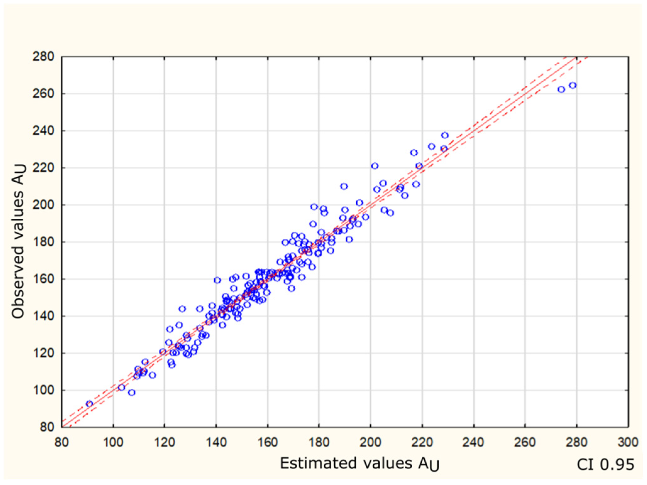
The first stage of modelling was the estimation of linear regression parameters for estimating the usable area of buildings based on a dataset from architectural offices. The initial dataset consisted of 191 one- and two-storey residential buildings with multi-pitched roofs. Figure 1 shows the relationship between the predicted and observed values for the dependent variable: the usable area (AU) of the building, for the last form of the linear model, considered to be optimal, after rejecting 8 outliers and resigning from the most insignificant variable—the boiler room (B). The goodness-of-fit of this model to the data is at the level of 95%.
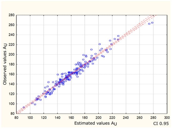
Figure 1.
Values observed in relation to the estimated usable area—circles. Red line is the trend line. The dashed line indicates the 95% confidence interval. Source: own calculation.
Each blue point represents a specific observation, with the horizontal axis (X) showing the usable area values predicted by the model and the vertical axis (Y) showing the actual observed values. The red solid and dashed lines are the regression line and the boundaries of the 95% confidence interval, respectively. Overlapping of the points and the regression line indicates the high reliability of the model. Most of the points are close to the regression line, which visually confirms that the model fits well with the data. The red line has a slope of about 45 degrees, which confirms that the predicted values are close to the observed values. The greater the deviation of the points from the regression line, the greater the estimate’s error.
Table 2 presents detailed results of multiple regression analysis for a sample of the final 183 observations, described by five independent variables (selected from Table 1). The values confirm the model being well fitted to the data (the coefficient of determination R2 with value 0.949 and adjusted R2 with value 0.947) and indicate that 95% of the variability of the usable area of the building is explained by the five independent variables. The variables covered area (AC), number of storeys (SN), and height (H) have a positive and significant impact on the usable area, which means that an increase in these values results in an increase in the usable area. The β weight (standardized regression coefficient), corresponding to the covered area, is as high as 1.105 and is the strongest estimator of the projected value of the usable area. The independent variable garage area (GA) has a negative effect on AU, which may be due to the fact that GA is not considered a usable area. The last two columns of Table 2 present the results of the significance test of the regression model parameters, namely the values of the test function t and the p-value; these confirm the high significance of all variables.
Table 2.
Multiple linear regression estimates for the building designs dataset. Source: own calculation.
Figure 2 illustrates the relative contribution of five different factors on a building’s usable area. The covered area is the most dominant factor (72%), which is consistent with the results presented in Table 2.
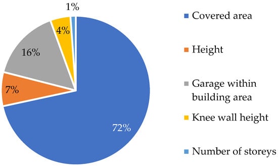
Figure 2.
Shares of independent variables in explaining the usable area of a building. Source: own calculation.
3.2. Nonlinear Regression Based on Building Designs
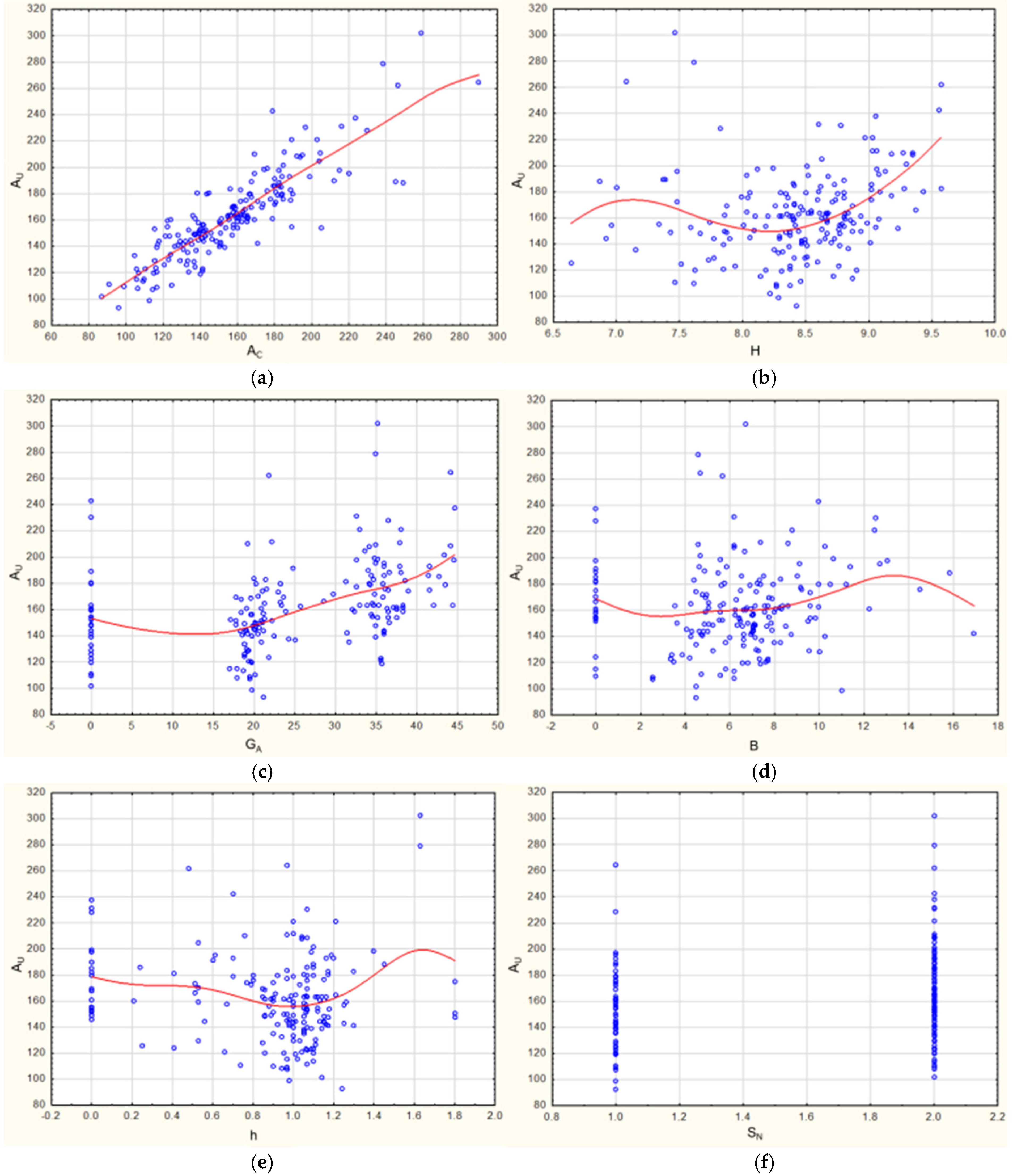
The construction of a nonlinear model began with the preparation of a series of scatterplots of the relationships between the dependent variable AU (usable area) and the independent variables (Figure 3a–f). A regression line, estimated using the least squares method, was added on each of the graphs (except for the two-valued variable SN) to illustrate the approximate type of AU dependence on a particular independent variable. Based on the regression lines, the mathematical functions for the independent variables were selected, from which a total and subsequently a final nonlinear regression model was built.
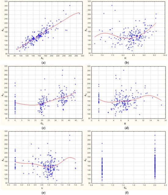
Figure 3.
(a–f) Dependence between usable area (AU) and independent variables. The blue circles indicate the values of the variables. Source: own calculation. (a) AU vs. AC (covered area). (b) AU vs. H (height). (c) AU vs. GA (garage area). (d) AU vs. B (boiler room). (e) AU vs. h (knee wall height). (f) AU vs. SN (number of storeys).
The tested functions that build the model (2) are shown in Table 3. Polynomial functions of degrees 1, 2, and 3 were tested. For a binary variable, the only possible function was a linear function. Finally, the additive multivariate model of nonlinear regression was formed (6):
where AU is the dependent variable, usable area of the building, a0 is the intercept of the nonlinear regression model, AC, H, GA, B, h, SN are the independent variables of the model (Table 3), bi, ci, di are model parameters.
Table 3.
Functions describing the dependence of the usable area on individual independent variables.
In the case of the nonlinear model, the analysis was performed similarly to the linear model. Parameter estimation was performed several times, which gradually eliminated the outliers and irrelevant independent variables. Table 4 presents the estimation of the parameters of the final form of nonlinear multiple regression considered to be optimal, which was based on 183 observations. Eight cases were considered to be the strongest outliers, seven of which also occurred as the strongest outliers in the linear model, which confirms their incompatibility with the analyzed dataset.
Table 4.
Multiple nonlinear regression estimates for the building designs dataset. Source: own calculation.
The model estimates the value of the usable area of the building based on several independent variables (AC, H, GA2, GA, h, SN). The value of the coefficient of determination R2 was 0.951 and its adjusted value was slightly lower (0.949). This means that 95% of the variability of the dependent variable is reliably explained by the model, indicating the very high fit of the model. The slight difference between R2 and its adjusted value confirms that the model remains stable even after accounting for the relationship between the number of data and the unknowns. The fit of the model is at the level of the linear model and the AC variable is again crucial in shaping the dependent variable.
The final form of the model includes independent variables with high significance, which are shown in the last two columns of Table 4. The regression model shows that most of the building characteristics included in the analyses were statistically significant in modelling (p-value < 0.05), with the exception of variable B (presence of the boiler room).
3.3. Linear and Nonlinear Models Based on the Existing Buildings in Koszalin
Multivariate regression models were constructed based on the database of 48 existing buildings in Koszalin, described by the same features that were assigned to the design dataset (Table 1). The estimation of model parameters followed the same logic as in the design dataset. In subsequent iterations of the estimation, the strongest outliers were removed individually. The significance of the independent variables was verified, with the aim of achieving the best possible fit of the model to the real data.
3.3.1. Linear Regression Based on Dataset of Existing Buildings
Table 5 presents the results of the estimation of the parameters of the best-fit linear regression model, form (1), without insignificant variables and without six outliers (explaining slightly more than 10% of the data).
Table 5.
Multiple linear regression estimates for the existing buildings’ dataset. Source: own calculation.
The linear multiple regression model has a high degree of fit to real data. The coefficient of determination is R2 = 0.919 and its adjusted value is slightly lower (Adj. R2 = 0.915), despite the fact that 12.5% of the data were considered outliers. This means that the model reliably explains about 92% of the actual dependence of the usable area of a building on its covered area and the number of storeys.
Both model independent variables (AC and SN) explain the dependent variable (AU) to a similar extent, as shown by β weights of 0.745 and 0.661, respectively. A detailed analysis of outliers showed that the rejected observations were indeed unusual for the adopted dataset. Some of them had a very large usable area or some did not have a garage or had an unusual roof shape. Thus, the empirical formula obtained from the estimation of the parameters of the linear multiple regression model takes the following form:
For a similar set of market data, Formula (7) may facilitate estimating the value of usable area on the local market.
3.3.2. Nonlinear Regression Based on Dataset of Existing Buildings
Table 6 presents the results of estimation of the parameters of the best fit among multivariate models of nonlinear multiple regression without five outliers, of which four were classified as outliers in the linear model.
Table 6.
Multiple nonlinear regression estimates for the existing buildings’ dataset. Source: own calculation.
The results of the nonlinear regression analysis indicate a very good (and slightly better than for a linear model) model fit. The coefficient of determination R2 reached 0.941 and its adjusted value was <1% lower (0.933), which indicates that the model reliably explains more than 93% of the dependence between variables. All independent variables left in the model were statistically significant. Each variable contributes to the explanation of the dependent variable at a similar level, as shown by the β weights, unlike in the design dataset.
The multivariate nonlinear regression model shows that the following variables are important estimators of the usable area of a building: covered area (AC), square of garage area (GA2), number of storeys (SN), square of the share of garage area in the building body (GP2), and share of garage area in the building body (GP).
Detailed analysis revealed that the rejected observations were objectively atypical in the adopted dataset. Some of them had a very large usable area or did not have a garage. The empirical formula obtained from the estimation of the nonlinear multiple regression model takes the form:
For a similar set of market data, also Formula (8), similarly to (7), may help property appraisers estimate the value of usable area on the local market.
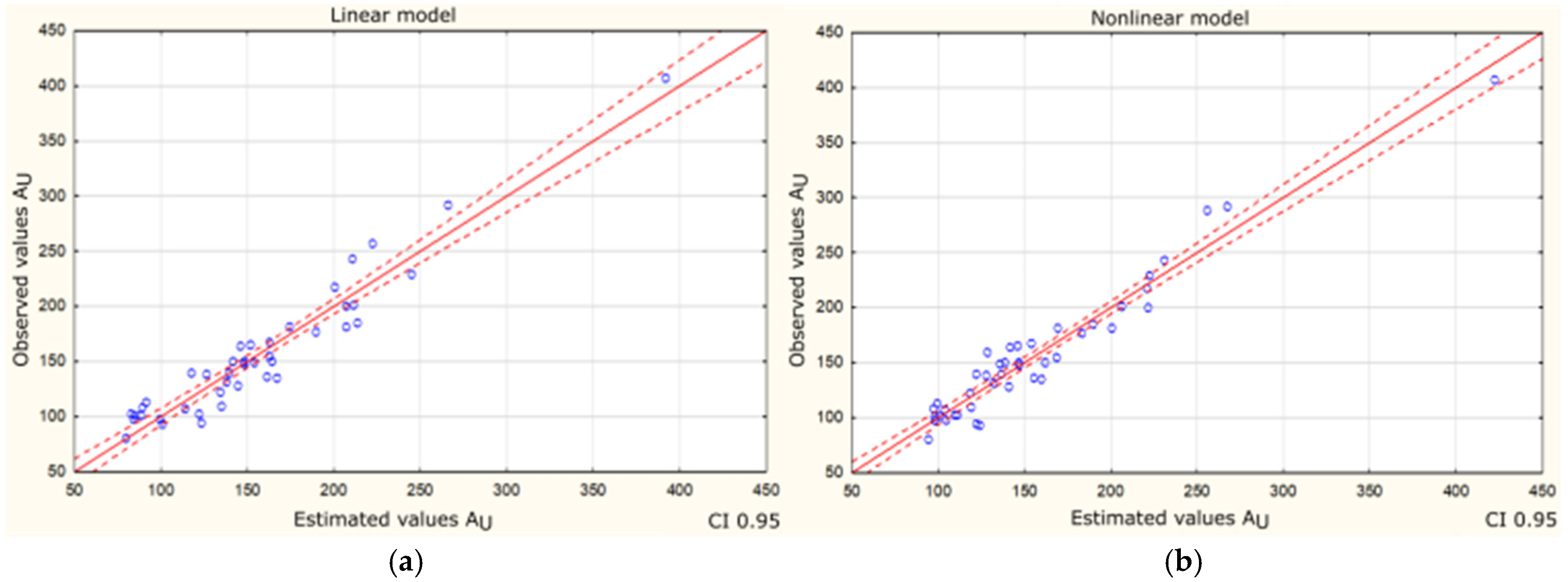
To visually compare the quality of forecasted models (linear and nonlinear) based on real data of existing building, plots of the dispersion of the observed values of the dependent variable in relation to its predicted values were created (Figure 4a,b).
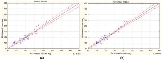
Figure 4.
Values observed in relation to the expected usable area of existing buildings dataset—circles. Red line is the trend line. The dashed line indicates the 95% confidence interval. Source: own calculation. (a) Linear model. (b) Nonlinear model.
Figure 4a,b are very similar and the points in both plots are relatively close to the regression line. The red dashed lines indicate the 95% confidence interval. For the nonlinear model, there is a slightly greater overlap of the predicted values of the usable area to the observed values of this variable; the points are more concentrated around the regression line and the determined confidence area. This is consistent with the evaluation of both models based on the coefficient of determination.
It can be stated that both types of models, linear and nonlinear, suitably reflect the dependence of the usable area on the selected characteristics of the building. Nevertheless, since the difference in the quality of fitting in favour of the nonlinear model is small (about 2%), the nonlinear model would probably be an easier tool in practical applications by property appraisers due to the simplicity of linear regression.
3.3.3. Prediction of Usable Area of Properties in a Test Set
The ultimate test of the model is its application in practice, while in the modelling process, the equivalent of such a practical test is the application of the model on data that were not used to determine the parameters of the model (validation). Such a validation of the models was performed in both cases. A comparison of the quality of the explanatory variable (estimates) obtained in this way is also an appropriate method of comparing the results of different models.
In the design dataset, another 10 observations were obtained on building designs that were not included in the model training group and a validation sample was created from them. A total of 201 observations were used throughout the process, including 191 in the training sample and 10 in the validation set. On the other hand, in the case of data on existing buildings in Koszalin, the dataset was divided into a set of 48 training observations and a validation set consisting of five elements already at the stage of data preparation. Thus, a total of 53 observations were used in the modelling process.
Each of the models obtained in Section 3.3.1 and Section 3.3.2 were verified by forecasting the usable area for the elements of the relevant validation test. Forecasts of the AU variable were determined and the results were summarized using MAE and RMSE measures. The results are presented in Table 7 and Table 8.
Table 7.
Quality of the estimation of the usable area for the validation test (N = 10) for the design data. Source: own calculation.
Table 8.
Quality of the estimation of the usable area for the validation test (N = 5) for the existing buildings data. Source: own calculation.
The A+ linear model showed the best predictive capabilities, and the B+ model is not much worse. Model B, described in Section 3.3.1, was slightly less successful in forecasting the area of new buildings. It should be noted that the validation sample itself included three observations, which accounted for most forecast errors. The remaining seven predictions were relatively accurate in each case.
In this case, the best predictions were obtained using Model C, indicated as the best in Section 3.3.2, followed by Model An and Model A. A significant part of the prediction errors was due to one observation in the validation set where the usable area was smaller than covered area by 15 m2 although this was a two-storey building. The house, however, has a double garage attached which affected the covered area. For the remaining objects, the usable area was estimated at a satisfactory level by most models.
3.3.4. Linear Models with LASSO Regularization
We have also performed a LASSO regularization in our analysis. The method is applied to linear models (cf. Formula (5)). The results are summed up in Table 9 and Table 10, for the design dataset and for the existing houses, respectively. The method allows for a selection of exogenous variables and one of our best regularized models indeed has the list of explanatory variables shortened to only three positions.
Table 9.
Quality of the estimation of the usable area for the validation test (N = 10) for the design data. Source: own calculation.
Table 10.
Quality of the estimation of the usable area for the validation test (N = 5) for the existing buildings data. Source: own calculation.
As we see in Table 9, the best predictions were obtained from the model minimizing the cross-validation error (λmin = 0.25), at least according to the RMSE measure. Hence, this model can be considered the best in his class. It is given by
After comparing with the previous models, we can conclude that the best regularized model for the design dataset is worse in terms of prediction accuracy than Model A+ described above.
Similarly, we estimated regularized models for the existing buildings dataset. Table 10 suggests that the best of the models obtained is not the model minimizing the penalty nor the model with or , but it is built with a larger value of . For , we obtain a model that has selected only three explanatory variables and performed best on out validation set:
After comparing Table 10 with Table 8, we can say that model with penalty parameter performed better on our validation sample than Model C described in Table 8. Hence, a LASSO regularized linear model proved to be the best model for this case in terms of prediction quality as it outperformed all linear and nonlinear models.
4. Discussion
In the case of the architectural design dataset, both linear and nonlinear models showed a very similar degree of fit and simultaneously eliminated the same number of outliers (4%) in subsequent iterations of parameter estimation. Nonlinear models offer advantages in the analysis of more complex dependences. However, in this case, the nonlinear model, although theoretically more flexible, did not bring clear benefits.
By analyzing the results, one can determine the importance of proper data processing before training the models. Atypical buildings, which are few in the random sample, cause a significant reduction in the accuracy of usable area estimates. Eliminating the knee wall variable in a nonlinear and linear model resulted in a reduction in the accuracy of predictions by only about 0.2%. This information is beneficial for property appraisers estimating the usable area of a building, as accurate measurement of this variable without entering the building is challenging and prone to significant error. However, on the other hand it may be crucial to know other parameters of the last storey instead, e.g., the slope of the roof planes can contribute to proper estimation of the overall usable area and it may be easier to collect. This will be further investigated in our future works.
In the case of the analysis of existing buildings in Koszalin, the linear and nonlinear models predicted the usable area similarly. The nonlinear multiple regression model, which was estimated after removing five outliers (10%), achieved a reliable value of R2 = 0.933. The best linear model was based on a set without six outliers (12.5%) and included only two significant variables (Ac and SN), which explained 91.5% of the variability in usable area. The difference in fit (<2%) is not substantial, and both models demonstrated a high and dependable alignment with the empirical data. In a nonlinear model, there is a greater number of variables that were important. In addition to Ac and SN, GA2, GP2, and GP were also significant. From a practical perspective, the linear model is more advantageous because it is inherently simpler and here it additionally operates with a smaller number of variables. The simplicity of this model is advantageous in that it allows for easier interpretation of the results and estimation of the usable area in practice.
We have stated above that if the nonlinear model is only slightly better fitted than the linear one, we prefer and advise the use of the linear model. However, whether the linear model will prove to be better than the nonlinear one cannot be reliably predicted beforehand and that is why we do evaluate nonlinear models as well. Still, the article provides only an illustration of how the modelling process can be organized in order to fill in the specific gaps in data. Every single analysis may be slightly different and there is a possibility that nonlinear models would prove to outperform their linear counterparts given certain circumstances. The computational complexity of such modelling is not a problem these days and practitioners do often consider multiple models before choosing one of them for use. We have proven that modelling usable area with a reasonable accuracy is possible using only a few characteristics of a building.
As buildings with multi-pitched roofs are a very heterogeneous group, special attention should be paid to data preparation for modelling purposes. The obtained models are prone to the occurrence of disparities in those areas of the domain in which the representation of objects in the training set is relatively scarce. It should also be noted that regression models can be used as an interpolation tool, understood as searching for the value of an endogenous variable for points that lie within the domain determined by the ranges of the exogenous variables, not outside of it. An attempt to estimate based on such models for atypical data will therefore be often unsuccessful. This occurred in the model validation process when some validation set elements came with strongly underrepresented feature combinations.
We have shown that the lacking data on usable area—a problem that concerns up to around 70% of the REPR data (according to previous research [15])—can be successfully addressed by means of relatively easy to use models that predict the usable area based on other characteristics of a building with a reasonable accuracy. Even if the models do not provide the same accuracy for all varying designs, for a majority of the typical houses, the estimation errors are acceptable. In the case of objects described by atypical sets of feature values, the errors are larger and that is natural, but we treat such cases as outliers and treat them separately. The estimated usable area in these cases has to be verified by an expert. And the more such verified cases there are in the database, the more accurately the model will behave during further use.
The final choice of the model depends on the nature of the available data and the purpose of the analysis. In this study, the linear model or the regularized linear model was a better tool for forecasting the usable area of a building from the perspective of property appraisers. The results are quite promising in terms of the accuracy of estimating the usable area in the context of their suitability for property valuation. The method is expected to be replicable in other regions of the country where the same legal framework and definition of usable area occurs; however, the model is fitted to the local data. A limitation of these studies is the lack of access to the interiors of existing buildings in Koszalin. This would have enabled identification of atypical building structures, such as the presence of high rooms in residential buildings, which is often associated with mezzanines. Such structures present challenges that are not easily addressed by regression models. Therefore, the next step in estimating the usable area in detached residential buildings with a multi-pitched roof will be the use of neural networks and machine learning methods. Further plans include reaching a larger database of properties and conducting an in-depth analysis, distinguishing more specific groups of buildings, measuring whether clustering can be used, i.e., automatic algorithms that divide objects into coherent, homogeneous classes, or whether it is an issue in which only expert knowledge will bring the desired results. The results from this, past, and future studies may find a practical implementation in form of an end-user friendly application.
The LiDAR-based data are accessible for many countries in the EU, thus the national sources can serve as a basis for similar analysis. We believe it is possible to adopt the method described in the article to other countries with the data accessible at hand, but further investigation is needed to prove the point. The architectural design data are representative for most of Poland (except for some mountainous areas, where roofs tend to be steeper). Our observations show that similar (in terms of shape) buildings are found in most neighbouring countries. And since only general building characteristics are used in the models, it seems that the use of such an approach may be even wider.
Researchers interested in replicable studies for their own countries are recommended to seek for the free LiDAR sources from EC report [44].
Author Contributions
Conceptualization, L.D.; methodology, L.D. and A.B.; validation, L.D., A.B., P.B., and U.A.-K.; formal analysis, L.D.; investigation, L.D., A.B., P.B., and U.A.-K.; resources, L.D., A.B., P.B., and U.A.-K.; data curation, L.D.; writing—original draft preparation, L.D. and A.B.; writing—review and editing, L.D., A.B., P.B., and U.A.-K.; visualization, U.A.-K.; supervision, L.D.; project administration, L.D. All authors have read and agreed to the published version of the manuscript.
Funding
Open access funding provided by University of Helsinki.
Institutional Review Board Statement
Not applicable.
Informed Consent Statement
Not applicable.
Data Availability Statement
The raw data supporting the conclusions of this article will be made available by the authors on request.
Acknowledgments
We thank Anna Dawid for the useful discussions.
Conflicts of Interest
The authors declare no conflicts of interest.
Abbreviations
The following abbreviations are used in this manuscript:
| BDOT10k | Database of Topographic Objects (pol. Baza Danych Obiektów Topologicznych) |
| LiDAR | Light Detection and Ranging |
| LoD | Level of Detail |
| REPR | Real Estate Price Register (pol. Rejestr Cen Nieruchomości) |
| MAE | Mean Absolute Error |
| RMSE | Root Mean Squared Error |
References
- Źróbek, S.; Bełej, M. Podejście Porównawcze w Szacowaniu Nieruchomości; Educaterra: Olsztyn, Poland, 2000. (In Polish) [Google Scholar]
- Hozer, J.; Kokot, S.; Kuźmiński, W. Metody Analizy Statystycznej Rynku w Wycenie Nieruchomości; PFSRM: Warszawa, Poland, 2002. (In Polish) [Google Scholar]
- Prystupa, M. Wycena Nieruchomości Przy Zastosowaniu Podejścia Porównawczego; PFSRM: Warszawa, Poland, 2001. (In Polish) [Google Scholar]
- Prystupa, M.; Brodaczewski, Z.; Szaraniec, G. Określanie wartości w zależności od ceny średnie. Rzeczozn. Majątkowy 2008, 58, 19. (In Polish) [Google Scholar]
- Rozporządzenie Ministra Rozwoju, Pracy i Technologii z Dnia 27 Lipca 2021 r. w Sprawie Ewidencji Gruntów i Budynków, Dz.U. 2021 poz. 1390. Available online: https://isap.sejm.gov.pl/isap.nsf/DocDetails.xsp?id=WDU20210001390 (accessed on 18 October 2024).
- Bydłosz, J. The application of the Land Administration Domain Model in building a country profile for the Polish Cadastre. Land Use Policy 2015, 49, 598–605. [Google Scholar] [CrossRef]
- Hycner, R. Basics of the Cadastre; AGH University of Science and Technology Press: Kraków, Poland, 2004; pp. 241–282. (In Polish) [Google Scholar]
- Dawidowicz, A.; Źróbek, R. A methodological evaluation of the Polish cadastral system based on the global cadastral model. Land Use Policy 2018, 73, 59–72. [Google Scholar] [CrossRef]
- Bennett, R. On the Nature and Utility of Natural Boundaries for Land and Marine Administration. Land Use Policy 2010, 27, 772–779. [Google Scholar] [CrossRef]
- Przewięźlikowska, A. Legal aspects of synchronising data on real property location in polish cadastre and land and mortgage register. Land Use Policy 2020, 95, 104606. [Google Scholar] [CrossRef]
- Kocur-Bera, K. Data compatibility between the Land and Building Cadaster (LBC) and the Land Parcel Identification System (LPIS) in the context of area-based payments: A case study in the Polish Region of Warmia and Mazury. Land Use Policy 2019, 80, 370–379. [Google Scholar] [CrossRef]
- Stendard, N.; Gilles, D.; Abdennadher, N.; Gallinelli, P. GPU-Enabled Shadow Casting for Solar Potential Estimation in Large Urban Areas. Application to the Solar Cadaster of Greater Geneva. Appl. Sci. 2020, 10, 5361. [Google Scholar] [CrossRef]
- Xu, B.; Han, Z.; Chen, M. Precise Cadastral Survey of Rural Buildings Based on Wall Segment Topology Analysis from Dense Point Clouds. Appl. Sci. 2023, 13, 10197. [Google Scholar] [CrossRef]
- Kokot, S. Data Quality of Transaction Prices in Real Estate Market. Acta Sci. Adm. Locorum 2015, 14, 43–49. (In Polish) [Google Scholar]
- Dawid, L. Analysis of Completeness of Data from the Price and Value Register on the Example of Kołobrzeg and Koszalin Districts in Years 2010–2017. Stud. Res. FEM SU 2018, 1, 91–102. (In Polish) [Google Scholar]
- Dawid, L. Analysis of Data Completeness in the Register of Real Estate Prices and Values Used for Real Estate Valuation on the Example of Koszalin District in the Years 2010–2016. Folia Oecon. Stetin. 2018, 18, 17–26. [Google Scholar] [CrossRef]
- Benduch, P.; Butryn, K. Legal and standard principles of buildings and their parts usable floor area quantity surveying. In Infrastructure and Ecology of Rural Areas; Polish Academy of Sciences: Cracow, Poland, 2018; pp. 225–238. ISSN 1732-5587. (In Polish) [Google Scholar]
- Benduch, P.; Hanus, P. The Concept of Estimating Usable Floor Area of Buildings Based on Cadastral Data. Rep. Geod. Geoinform. 2018, 105, 29–41. [Google Scholar] [CrossRef]
- Budzyński, T. Calculating the Area of Newly-Built Apartments and Buildings According to Uniform Rules. Geod. R. 2012, 84, 31. (In Polish) [Google Scholar]
- Buśko, M. Analysis of legal and Proposed Changes in Definition of Contour of Building in Real Estate Cadastre. Geomat. Environ. Eng. 2018, 12, 29–44. [Google Scholar] [CrossRef]
- Ebing, J. Calculating of Area and Cubic Volume of Facilities with Different Intended Use; Verlag Dashofer Sp. z o.o Publishing House: Ljubljana, Slovenia, 2011; ISBN 978-83-7537-108-6. (In Polish) [Google Scholar]
- PN-70/B-02365; Surface Area of Buildings—Classification, Definitions, and Methods of Measurement. Polish Committee of Standardization: Warszawa, Poland, 1970. Available online: http://rzeczoznawca-zachodniopomorskie.pl/pliki/PN_70_B_02365.pdf (accessed on 22 April 2022). (In Polish)
- PN-ISO 9836:1997; Performance Standards in Building—Definition and Calculation of Area and Space Indicators. Polish Commitee of Standardization: Warszawa, Poland, 1997. Available online: http://rzeczoznawca-zachodniopomorskie.pl/pliki/PN_ISO_9836_1997.pdf (accessed on 20 April 2022). (In Polish)
- Regulation of the Minister of Transport, Construction and Maritime Economy of April 25, 2012 on Detailed Scope and Form of a Construction Project. Journal of Laws of 2012, Item 462. Available online: https://isap.sejm.gov.pl/isap.nsf/DocDetails.xsp?id=wdu20120000462 (accessed on 20 May 2020). (In Polish)
- PN-ISO 9836:2015-12; Performance Standards in Building—Definition and Calculation of Area and Space Indicators. Polish Commitee of Standardization: Warszawa, Poland, 2015. Available online: https://sklep.pkn.pl/pn-iso-9836-2015-12p.html (accessed on 18 October 2024). (In Polish)
- Dawid, L.; Tomza, M.; Dawid, A. Estimation of usable area of flat-roof residential buildings using topographic data with machine learning methods. Remote Sens. 2019, 11, 2382. [Google Scholar] [CrossRef]
- Zbroś, D. The Rules for Calculating the Usable Area by Two Current Polish Standards. Saf. Eng. Anthropog. Objects 2016, 3, 19–22. (In Polish) [Google Scholar]
- Database of Topographic Objects (pol. Baza Danych Obiektów Topologicznych) (BDOT). Available online: https://www.geoportal.gov.pl/pl/dane/baza-danych-obiektow-topograficznych-bdot10k/ (accessed on 10 September 2024).
- Wężyk, P. (Ed.) Textbook for Participants of Trainings on Using LiDAR Products; Head Office of Land Surveying and Cartography: Cracow, Poland, 2015. (In Polish) [Google Scholar]
- Ren, X.; Yu, B.; Wang, Y. Semantic Segmentation Method for Road Intersection Point Clouds Based on Lightweight LiDAR. Appl. Sci. 2024, 14, 4816. [Google Scholar] [CrossRef]
- 2.0; CityGML. Open Geospatial Consortium: Arlington, TX, USA, 2012.
- Barańska, A. Linear and Nonlinear Weighing of Property Features. Real Estate Manag. Valuat. 2019, 27, 59–68. [Google Scholar] [CrossRef]
- Baldominos, A.; Blanco, I.; Moreno, A.J.; Iturrarte, R.; Bernárdez, Ó.; Afonso, C. Identifying Real Estate Opportunities Using Machine Learning. Appl. Sci. 2018, 8, 2321. [Google Scholar] [CrossRef]
- Kim, J.; Lee, Y.; Lee, M.-H.; Hong, S.-Y. A Comparative Study of Machine Learning and Spatial Interpolation Methods for Predicting House Prices. Sustainability 2022, 14, 9056. [Google Scholar] [CrossRef]
- Dawid, L.; Cybiński, K.; Stręk, Ż. Machine Learning of Usable Area of Gable-Roof Residential Buildings Based On Topographic Data. Remote Sens. 2023, 15, 863. [Google Scholar] [CrossRef]
- Dudzik, P. Geometria dachów (Roof geometry). Inżynieria I Bud. 2023, LXXIX, 293–298. [Google Scholar]
- Lipińscy, M.L. Design Office. Houses Projects. Available online: https://lipinscy.pl/ (accessed on 21 May 2024).
- Mendel, B. ARCHON+ Project Office. Available online: https://www.archon.pl/ (accessed on 21 May 2024).
- QGIS Development Team. QGIS Geographic Information System. Open Source Geospatial Foundation Project. Available online: http://qgis.osgeo.org (accessed on 21 May 2024).
- Head Office of Land Surveying and Cartography. Geoportal of National Spatial Data Infrastructure. Available online: https://www.geoportal.gov.pl/ (accessed on 12 May 2024).
- Barańska, A. Statystyczne Metody Analizy i Weryfikacji Proponowanych Algorytmów Wyceny Nieruchomości; AGH publishing: Kraków, Poland, 2010. [Google Scholar]
- Santosa, F.; Symes, W.W. Linear inversion of band-limited reflection seismograms. SIAM J. Sci. Stat. Comput. 1986, 7, 1307–1330. [Google Scholar] [CrossRef]
- Tibshirani, R. Regression Shrinkage and Selection via the lasso. J. R. Stat. Soc. Ser. B (Methodol.) 1996, 58, 267–288. [Google Scholar] [CrossRef]
- Kakoulaki, G.; Martinez, A.; Florio, P. Non-Commercial Light Detection and Ranging (LiDAR) Data in Europe; Publications Office of the European Union: Luxembourg, 2021; ISBN 978-92-76-41150-5. EUR 30817 EN. [Google Scholar] [CrossRef]

Disclaimer/Publisher’s Note: The statements, opinions and data contained in all publications are solely those of the individual author(s) and contributor(s) and not of MDPI and/or the editor(s). MDPI and/or the editor(s) disclaim responsibility for any injury to people or property resulting from any ideas, methods, instructions or products referred to in the content. |
© 2024 by the authors. Licensee MDPI, Basel, Switzerland. This article is an open access article distributed under the terms and conditions of the Creative Commons Attribution (CC BY) license (https://creativecommons.org/licenses/by/4.0/).