Abstract
The rapid growth of cities and their populations in recent years has resulted in significant tidal passenger flow characteristics, primarily manifested in the imbalance of passenger numbers in both directions. This imbalance often leads to a shortage of train capacity in one direction and an inefficient use of capacity in the other. To accommodate the tidal passenger flow demand of urban rail transit, this paper proposes a timetable optimization method that combines multiple strategies, aimed at reducing operating costs and enhancing the quality of passenger service. The multi-strategy optimization method primarily involves two key strategies: the unpaired operation strategy and the express/local train operation strategy, both of which can flexibly adapt to time-varying passenger demand. Based on the decision variables of headway, running time between stations, and dwell time, a mixed integer linear programming model (MILP) is established. Taking the Shanghai Suburban Railway airport link line as an example, simulations under different passenger demands are realized to illustrate the effectiveness and correctness of the proposed multi-strategy method and model. The results demonstrate that the multi-strategy optimization method achieves a 38.59% reduction in total costs for both the operator and the passengers, and effectively alleviates train congestion.
1. Introduction
The rail system is usually the first choice for traveling in people’s daily lives because of its punctuality and convenience. Taking the passenger flow of the Shenzhen Metro’s urban rail transport in China as an example, the Automatic Fare Collection (AFC) system recorded over 140 million transactions over a period of 48 days [1]. At the same time, the maximum number of trains running on weekdays is nearly seven thousand. If the timetable is planned appropriately while still satisfying passenger demand, significant unnecessary costs will be minimized [2].
Passenger demand in the railway system is characterized by spatial and temporal imbalances. Therefore, many researchers have studied the impact of passenger demand on the train scheduling process. From the perspective of time-dependent passenger demand, a variable train composition method was implemented [3,4]. Moreover, a non-fixed headway between two consecutive trains is achieved, which allows the system to adapt to passenger demand levels that vary with the peak and off-peak hours [5,6]. Based on the current research focus, spatial passenger demand can be categorized into two types: passenger flow demand at different stations and passenger flow demand in different directions. When there is frequent congestion at certain stations, implementing a skip-stop strategy and an appropriate stopping scheme can effectively alleviate platform congestion [7,8,9,10]. The implementation of a skip-stop strategy can save energy consumption and maintenance costs [11].
In addition, the express/local train operation strategy (ELS) is also a common approach to solving the problem of station congestion [12,13]. The ELS can speed up the cycle running time by adjusting the skip-stop behavior of express trains, and also ensure that passengers waiting on the platform can board the trains smoothly using the all-stop behavior of local trains. Due to urban development, passenger flow in commercial center stations far exceeds that of other stations. The short-turning strategy is adopted to increase the number of trains running in the commercial center section [6,14,15]. The above studies are about the imbalance of passenger flow at stations, and it is worth noting that passenger flow imbalances in opposing directions are often caused by the tidal passenger flow phenomenon [16]. However, studies on passenger flow imbalances in opposite directions are minimal.
According to passenger travel patterns during morning peak hours, the number of people traveling from the suburbs to the city center is significantly higher than those traveling in the opposite direction. However, during the evening rush hour, many people who work and study near the city center return to their suburban homes, resulting in the tidal passenger flow phenomenon [17]. To cope with the problem, this paper proposes a train unpaired operation strategy (TUOS), i.e., the number of trains running in both directions is not the same. Compared to the traditional train paired operation strategy (T-TPOS) [3,18,19], the TUOS improves the matching of passenger numbers and train capacity by flexibly determining the number of trains in both directions.
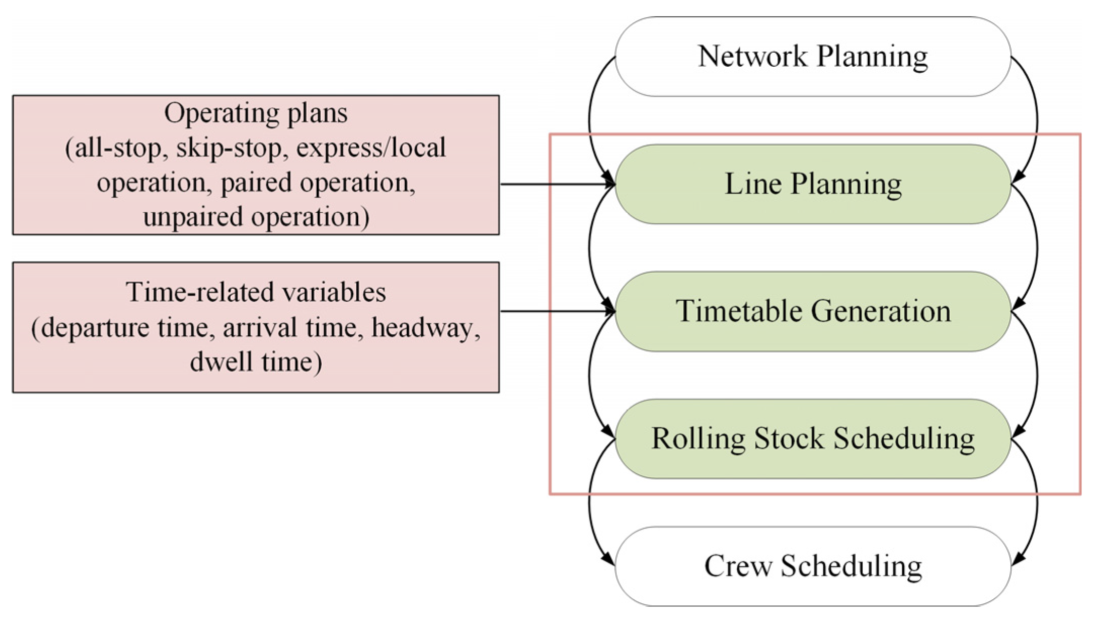
The above discussed is the Line Planning level of the rail transport planning process [20,21]. As shown in Figure 1, after the Line Planning level, the Timetable Generation level should be entered. In other words, the Timetable Generation level is the confirmation of train departure time, arrival time, headway, and dwell time. Timetable optimization considering rolling stock scheduling is the focus of our current research, which takes into account the quality of passenger service as well as the cost of operating trains [19,22]. Therefore, this paper selects three processes in the rail transport planning process for research, which are the Line Planning level, Timetable Generation level, and Rolling Stock Scheduling level.

Figure 1.
The rail transport planning process.
Usually, timetable optimization is conducted with the objective of improving passenger service quality and reducing operating costs. Passenger service quality is generally defined as total passenger waiting time [23,24], total passenger travel time [16,25], number of stranded passengers [20], etc. The operator’s operating costs include train operating expenses and train stopping expenses.
So far, few studies have focused on the TUOS. Compared to TUOS, the T-TPOS offers significant advantages in transport organization, but it can lead to a waste of resources due to the lack of passengers in a certain direction in the face of a tidal passenger flow scenario. Therefore, we use the tidal passenger flow phenomenon as a background to achieve optimization of a timetable. It is noteworthy that the TUOS allows for a flexible allocation of trains in both directions, whereas the ELS can manage stopping schemes and accelerate the cycle running time of trains. However, this paper selects the combined strategies of unpaired operation and express/local train operation, abbreviated as the TUOS-ELS, which is a multi-strategy operation method.
This paper considers three planning processes of the rail transport planning process, namely the Line Planning level, Timetable Generation level, and Rolling Stock Scheduling level. A multi-strategy optimization method, which will contribute to the future development of rail transit systems, is developed. The highlights of this paper are as follows:
- Based on the tidal passenger flow phenomenon, a TUOS-ELS is proposed in this paper, consisting mainly of TUOS and ELS. In TUOS, the total number of trains running in both directions is determined. In ELS, according to passenger flow data, the stops express trains will skip are selected. Rolling stock circulation is also considered.
- The nonlinear model related to timetable and passenger flow is linearized, and the objectives of minimizing the number of stranded passengers, the total travel time of all trains, and the total number of stops are set. A multi-objective mixed integer linear programming (MILP) model is constructed to achieve an exact solution within a reasonable computational time. The optimization procedure is designed according to the actual train operation process, and the GUROBI solver is used to solve the optimization problem.
- Based on the Shanghai Suburban Railway airport link line, timetable optimization under different passenger flow scenarios is investigated, and the optimization results of the TUOS-ELS and T-TPOS are compared.
The rest of the paper is organized as follows. In Section 2, we provide a detailed description of the research question. In Section 3, we establish the train traffic dynamic model and passenger flow model. The MILP model is constructed by linearizing the nonlinear constraints. In Section 4, we design the optimization procedure. In Section 5, two case analyses based on the Shanghai Suburban Railway are provided to illustrate the correctness and effectiveness of the proposed method and model. Finally, we conclude this study in Section 6.
2. Problem Description
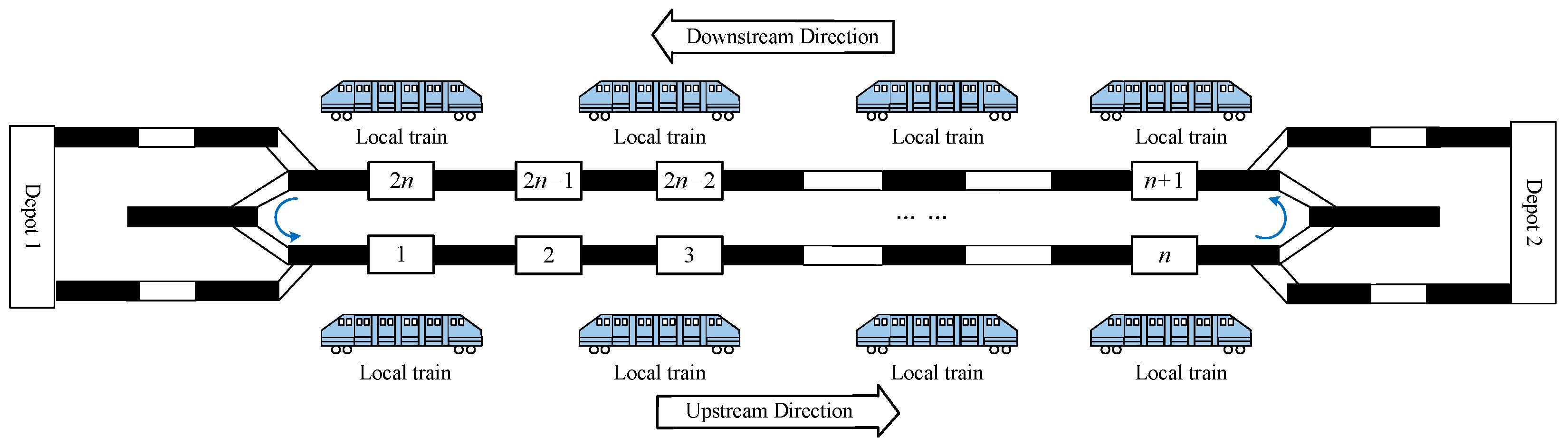
A crowded railway line linking the city center to the suburbs is studied in this paper, as shown in Figure 2 and Figure 3. S is used to represent the stations where the trains will perform the task of loading passengers, i.e., .
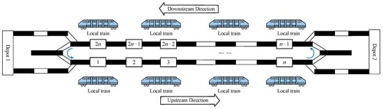
Figure 2.
Illustration of train operation under T-TPOS.
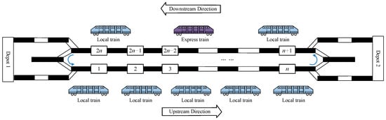
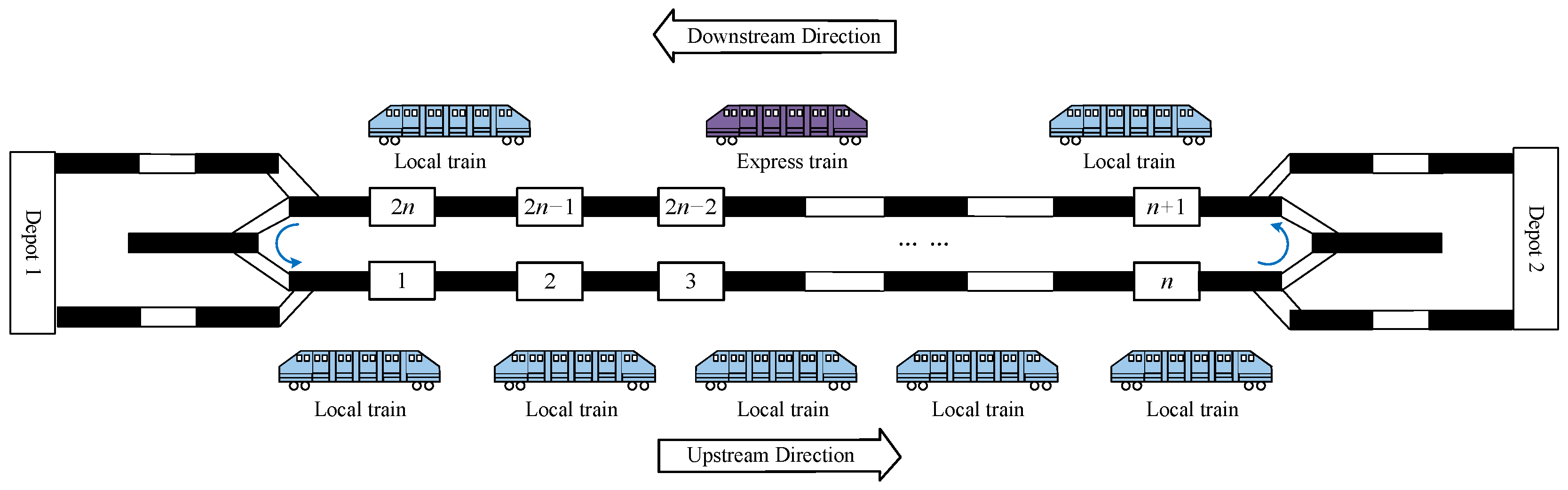
Figure 3.
Illustration of train operation under TUOS-ELS.
In Figure 2, it is obvious that the number of trains running in both directions is the same, following the strategy called the T-TPOS. The T-TPOS embodies the advantages of being simple and easy to realize, but it also has many shortcomings when dealing with the problems caused by tidal passenger flow. If T-TPOS is implemented on tidal passenger flow lines, the total train capacities in the upstream direction (i.e., the main passenger flow direction) will not be able to meet the passenger demand and will lead to the waste of train utilization in the downstream direction (i.e., the non-main passenger flow direction).
In order to solve the problem of uneven distribution of passenger numbers in opposing directions, timetable optimization based on the TUOS-ELS is studied to enhance the matching of train capacity and passenger demand. In Figure 2, the total number of trains running in both directions is eight. With the same total number of trains running, the TUOS-ELS in Figure 3 is adopted, where five trains operate closely in the upstream direction and three trains operate sparsely in the downstream direction. The flexible number of trains and the headway between two consecutive trains can accommodate uneven passenger demand. In addition, the determination of the number of trains plays an important role. The ELS is executed in the downstream direction, and the express trains can shorten the travel time from the first station to the terminal station. However, there are local trains running in both directions, maintaining all-stop behavior to ensure service quality. All-stop behavior means that the train stops at every station it passes through.
This paper considers both passenger service quality and operating costs. When passengers wait on the platform, they only care about whether they can board the upcoming train and their travel time. Therefore, the number of stranded passengers on the platform and travel time of trains were chosen as indicators of service quality. The stopping costs were selected as operating costs. To conclude, this paper adopts a multi-strategy operation method and constructs a multi-objective MILP model to optimize the timetable, aiming to minimize the total number of stops, the number of stranded passengers, and the total travel time of trains.
This paper focuses on the study of timetable optimization. The number of trains, the running time between stations, the dwell time, the departure time, and the passenger’s traveling behavior are considered. To simplify the model, the proposed assumptions are illustrated as follows:
Assumption 1.
Urban rail lines do not provide sidings, do not support temporary train additions and subtractions, and do not support overtaking operations at any location on the line.
Assumption 2.
Passengers can be informed of stations where the upcoming train will not stop through their mobile devices as well as platform announcements. Passengers may only travel on trains that are valid for them, i.e., trains that stop at both the passenger’s origin and destination, and that do not take into account the passenger’s transfer behavior.
Assumption 3.
To simplify the passenger waiting model, it is assumed that the waiting passengers of different OD (Origin-Destination) pairs are mixed at the platform. When the train reaches the platform, the number of stranded passengers is random.
3. Mathematical Modeling
In this section, due to the necessity of clearly indicating the relationships between the timetable and passengers’ boarding and alighting behavior, a train traffic dynamic model and a passenger flow model are developed and detailed conceptual descriptions are given. A MILP model is constructed by linearizing the nonlinear components, which facilitates an accurate solution to the problem.
3.1. Train Traffic Dynamic Model
The headway between two consecutive trains i and i-1 determines the number of waiting passengers at station s. Setting an appropriate headway will avoid the problem of the number of waiting passengers exceeding the available platform capacity during peak periods and solve the problem of wasted train capacity.
where and are the maximum and minimum headway, respectively. I is the set of train serial numbers in both directions, and the number of trains running is determined by the number of passengers. and are the total number of trains running in the upstream and downstream directions respectively.
It should be clear how the number of trains is determined. The minimum number of trains is obtained based on the ratio of the expected maximum number of on-board passengers. The expected maximum number of on-board passengers is calculated with the maximum headway and train capacity C assumed to be infinite. The minimum number of trains during the study period should also satisfy the maximum headway constraint, as shown in Equation (2). After that, the maximum number of trains can be determined by calculating the minimum headway, as shown in Equation (3).
where is the number of on-board passengers of the train i leaving station s. After obtaining the maximum/minimum number of trains in both directions, the upper and lower bound constraints on the actual number of trains can be acquired, i.e., .
The departure time of train i at station s is related to the arrival time and dwell time , where the arrival time is composed of the departure time at the previous station s-1 and the running time from station s-1 to station s of train i, as shown in Figure 4.
where indicates whether the train i stops at station s. If the train i stops at station s, , otherwise . The terms and are the minimum dwell time and maximum dwell time of the train i at station s. The terms are the minimum running time and maximum running time of the train i from station s-1 to station s.
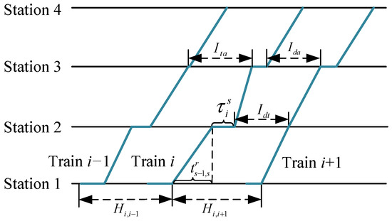
Figure 4.
Description of train running status.
In order to guarantee service quality, this paper specifies two train skip-stop behaviors. On the one hand, when three consecutive trains pass the same station s, at least two trains stop at station s, i.e., three consecutive trains are not allowed to skip the same station. On the other hand, a train cannot skip three consecutive stations.
In Figure 4, the time constraints are more clearly reflected. Considering an example involving three trains across four stations, train i-1 skips station 3, train i chooses to stop at all stations, and train i + 1 skips station 2.
Since the safe operation of trains is very important, the departure time of train i at station 3 and the arrival time of train i + 1 at station 3 should satisfy the “departure-arrival” time constraint , i.e., the first constraint in Equation (10). The departure time of train i at station 2 and the arrival time of train i + 1 at station 2 should satisfy the “departure-passing” time constraint , i.e., the third constraint in Equation (10). The arrival time of train i at station 3 and the departure time of train i − 1 at station 3 should satisfy the “passing-arrival” time constraint , i.e., the second constraint in Equation (10).
The rolling stock operation constraints are mainly reflected in the train connection relationship and the turnaround operation time. A train can be connected to no more than one other train during its operational cycle:
where , are binary variables. If the train i in the upstream direction produces a rolling stock connection with the train j in the downstream direction, the is taken as 1, otherwise the is taken as 0. If the train j in the downstream direction produces a rolling stock connection with the train i in the upstream direction, the is taken as 1, otherwise the is taken as 0. is the set of train serial numbers in the upstream direction. is the set of train serial numbers in the downstream direction.
Two trains can be connected only if the connecting time between trains meets the minimum turnback time requirement:
where M is a positive maximum value.
The rolling stock connection affects the number of times rolling stock exits and enters the depot. The fewer times, the lower the operator’s operating costs.
where are binary variables. If the rolling stock of the train i and j does not enter the depot, and are 1, otherwise and are 0. If the rolling stock of trains i and j does not come from the depot, and are 1, otherwise and are 0.
3.2. Passenger Flow Dynamic Model
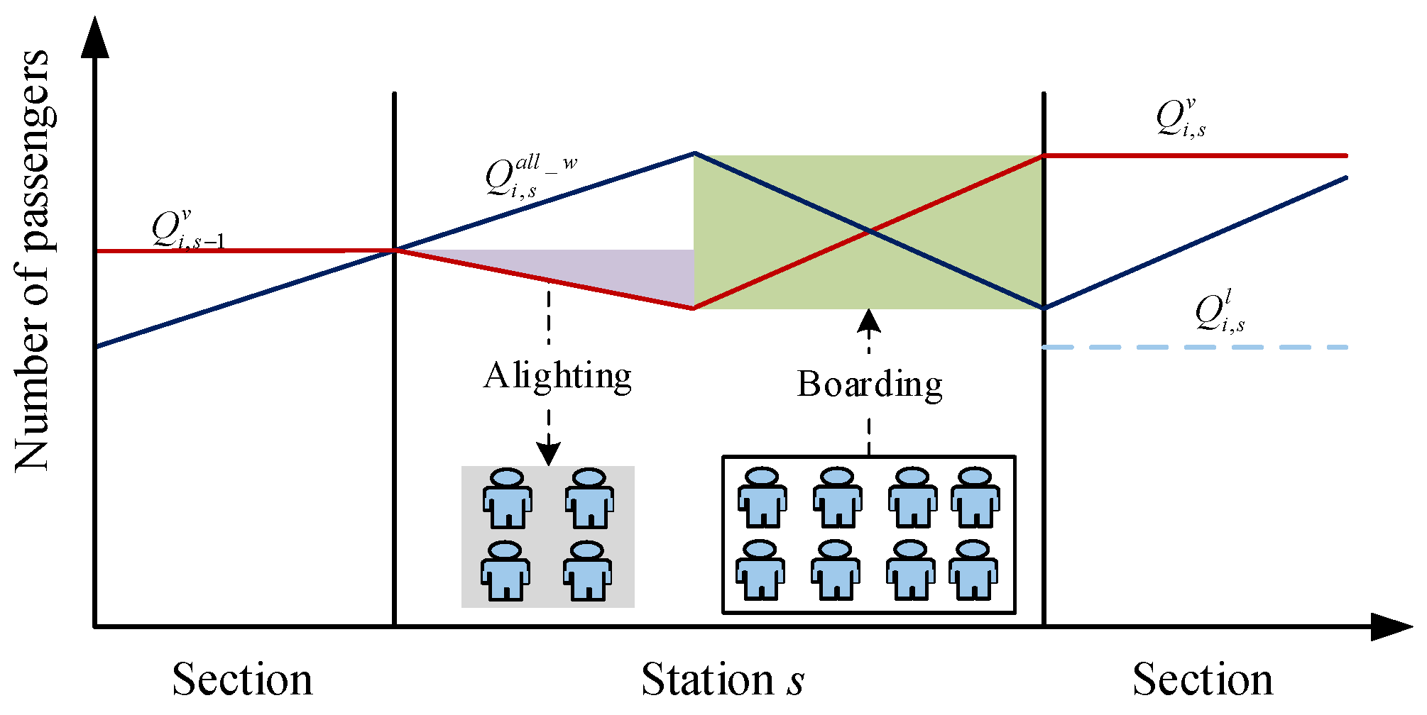
To illustrate the passenger-station interaction, Figure 5 was plotted. When a train is running between stations, the number of passengers waiting on the platform increases with the number of new passengers arriving until passenger loading actions take place. However, the number of on-board passengers varies as passengers alight and board.
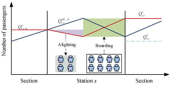
Figure 5.
Diagram of dynamically varying passenger flows.
Taking into account the time-varying passenger demand, it is critical to divide the time interval to accurately count passenger arrivals. By using the passenger arrival rate at station s during the time interval and the OD arrival ratio matrix , the number of passengers arriving at station s going to station k () between the departures of two consecutive trains can be calculated.
The total number of passengers waiting on station s toward destination k () is the combination of the stranded passengers of the previous train () and the newly arriving passengers .
where is the total number of passengers waiting for train i at station s. Moreover, according to Assumption 2, the number of passengers who want to board the train i at station s toward destination k is affected by the skip-stop action. The valid number of passengers waiting , is described as follows:
where is the total valid number of passengers waiting for train i at station s.
During peak hours, the actual number of passengers boarding the train i at station s () is related to the number of valid passengers waiting at station s () and the remaining capacity of train i at station s (). The actual number of passengers alighting at station s () is the total number of passengers who boarded the train i at other stations before station s and want to alight at station s.
where is the number of passengers successfully boarding train i from station m with destination station s. is the number of on-board passengers of the train i leaving station s-1.
By the description of the number of passengers alighting in Equation (19), it is obvious that the number of passengers successfully boarding train i from station s with destination station k () must be obtained. Based on assumption 3, all passengers were mixed on the platform to wait for the train i, which is consistent with the actual situation. To simplify the calculations, the number of passengers who successfully board the train i is proportional to the valid number of passengers waiting.
The number of passengers stranded by train i at station s who want to travel to station k () is given by the following.
where is the total number of passengers stranded by train i on station s.
3.3. Linearization of the Model
When optimizing a timetable, the train traffic dynamic model and passenger flow dynamic model are linearized to build a MILP model. From Equations (1) and (4)–(25), it can be found that Equations (10), (17), (22) and (23) are nonlinear constraints.
Equation (10) can be rewritten in the following nonlinear constraint form:
Introducing a binary variable transforms Equation (26) into Equation (27):
Similarly, the nonlinear Equation (17) can be transformed into the following linear constraint form:
The total number of passengers boarding the train i at station s is calculated by Equation (22), and the binary variable is introduced to represent the relative size relationship between and . If , then is equal to 1. Otherwise, is equal to 0.
Equation (23) can be converted to the following linear constraint form:
where is calculated when the train adopts the all-stop behavior as well as a fixed headway, dwell time, and running time between stations, i.e.,. is the valid number of passengers waiting at station s who are eager to travel to station k under the all-stop behavior, and is the total valid number of passengers waiting at station s under the all-stop behavior.
3.4. Problem Model
MILP is widely applied in studies related to timetable optimization [15,26,27]. MILP defines that the objective function, equation, and inequality constraints in an optimization problem are linear. Moreover, there must exist integer variables for the decision variables. The standard form of MILP is described by Equation (31).
where is the linear objective function. is the linear inequality constraint. is the linear equation constraint. is the boundary constraint. The term is an integer variable. The term is a logistic variable.
In the MILP model, four decision variables are considered, including the headway at the first station, the stop time at each station, the travel time between stations, and a binary variable indicating whether a train stops at a station, which can be represented by the matrix x.
where H matrix is the composed according to , with representing the total number of trains and n representing the number of stations. matrix is the consisting of . and A matrix are consisting of and respectively.
Based on the train traffic dynamic model and passenger flow dynamic model, according to the form of Equation (31), the multi-objective MILP problem is established as in Equation (33). Enhancing passenger service quality and reducing operating costs are the objectives in urban rail transport. The linear optimization objective function mainly considers stopping costs, the number of stranded passengers on the platform, and total train traveling time in both directions.
where are cost conversion factors for uniform magnitude. The term is the unit cost of a train stop. The term is the unit penalty cost of a stranded passenger. The term is the unit operating cost per second of a train.
4. Method
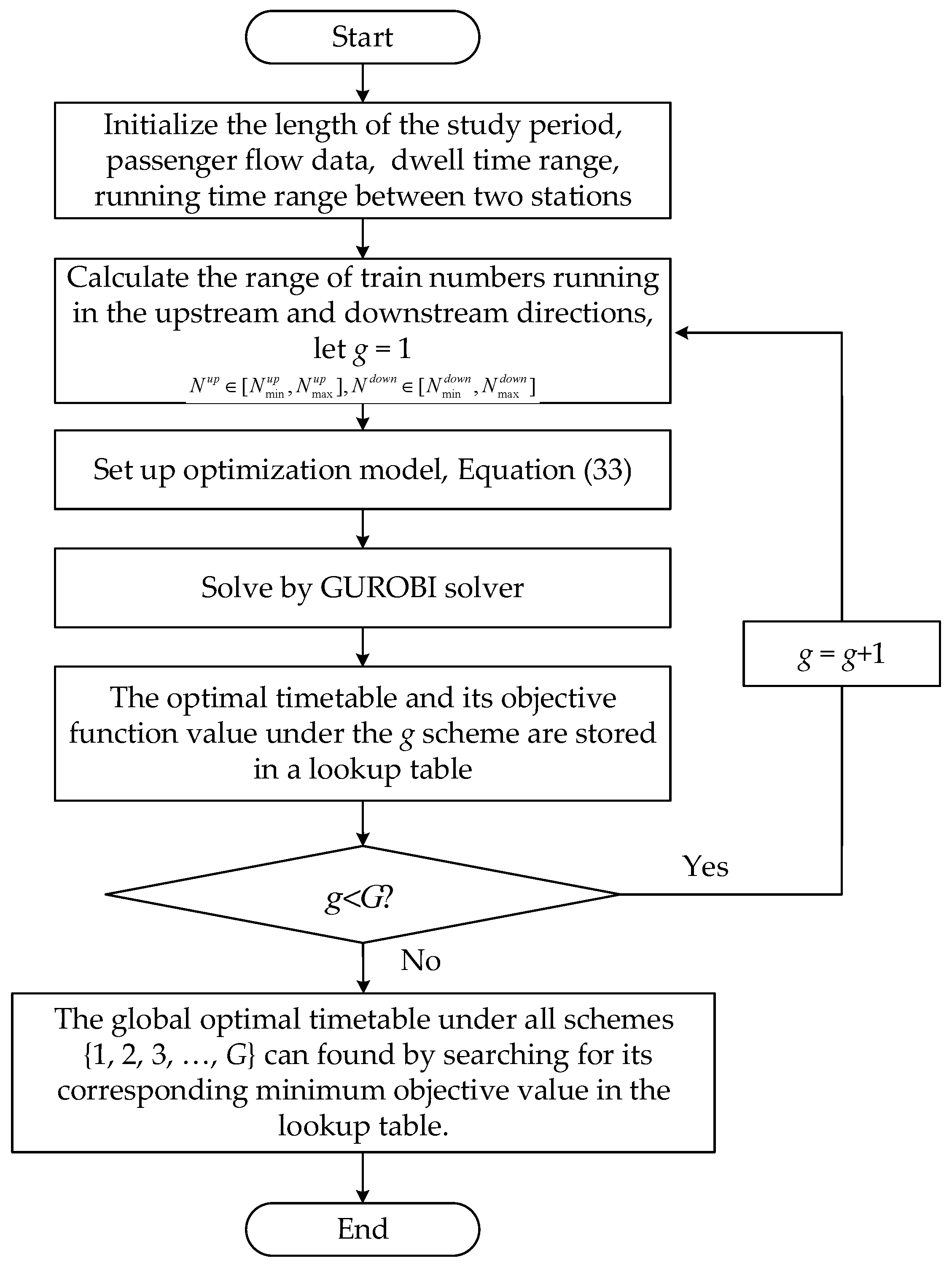
The optimization procedure is taken to solve the optimization problem, as illustrated in Figure 6. For a certain number of bi-directional trains, setting up its corresponding multi-objectives function and constraints, the minimized objective function value and timetable can be solved and stored in a lookup table. By traversing the different number of bi-directional trains, all the local optimal solutions are filled into the lookup table. The global optimal timetable can be found by searching for its corresponding minimum objective value in the lookup table.
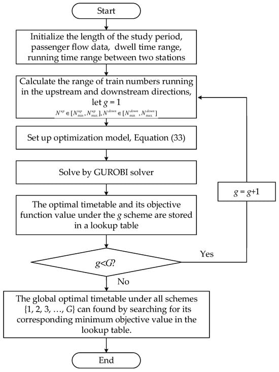
Figure 6.
The optimization procedure for solving the optimization problem.
In Figure 6, the steps of the optimization procedure are described. First, the ranges of the decision variables and the passenger flow data are specified. Second, the number of trains running in the upstream and downstream directions is calculated according to Equations (2) and (3). All of the possible combinations of the number of bi-directional trains are enumerated and indexed by g = {1, 2, 3, …, G}, with G representing the total number of combinations. The corresponding train numbers for each combination g are used as inputs to the optimization model during the optimization process. The optimization model refers to a mathematical representation used to solve an optimization problem and find the best solution based on specific objectives and constraints, i.e., Equation (33), which can be solved using the GUROBI solver of MATLAB. The optimization model is set up through YALMIP/MATLAB programming. Then, the timetable and objective function value obtained under the g scheme are stored in the form of a lookup table. Finally, based on the objective function values and timetables calculated for all schemes {1, 2, 3, …, G}, the global optimal timetable can be determined by searching the lookup table.
5. Case Study
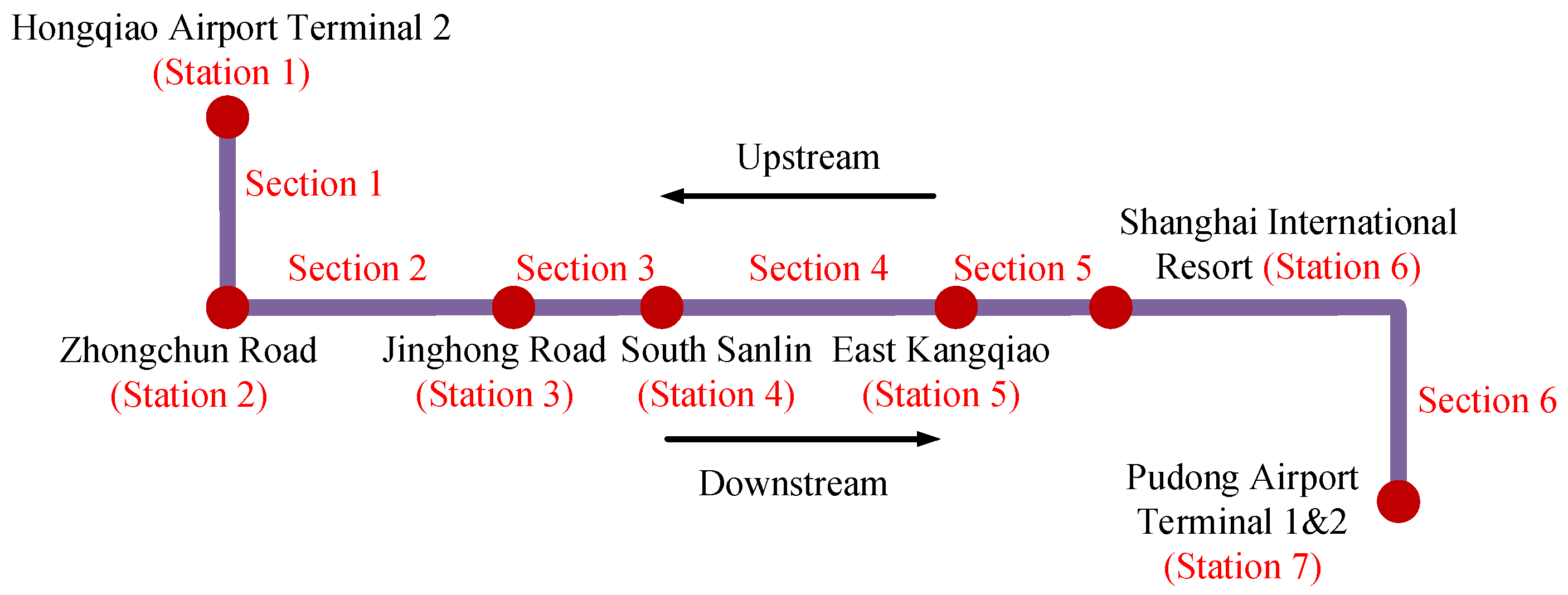
In this section, a simulation analysis is conducted based on the given passenger flow data and actual line data. In this paper, a Shanghai Suburban Railway airport link line, containing seven stations and six sections, was selected as the research object, as shown in Figure 7. It mainly involves Hongqiao Airport Terminal 2, Zhongchun Road, Jinghong Road, South Sanlin, East Kangqiao, Shanghai International Resort, and the Pudong Airport Terminal 1 and 2 stations. Since Pudong Airport Terminal 1 and 2 is a suburban station and Hongqiao Airport Terminal 2 is an urban station, the number of passengers traveling in the upstream direction far exceeds that in the downstream direction during the morning peak period [8:00, 9:00].
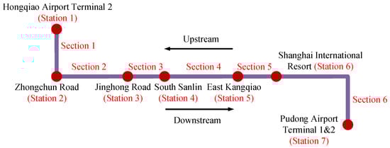
Figure 7.
The Shanghai Suburban Railway airport link line.
5.1. Simulation Setting
From the time-varying passenger arrival rate at stations shown in Figure 8, it can be observed that during the period from 6:00 to 9:00, the arrival rate at all platforms increased due to commuting reasons, reaching a peak between 8:00 and 9:00. Specifically, the passenger flow data used in this paper is derived from the compilation of literature [28]. It should be noted that the study applies to all urban rail transit lines that experience the tidal passenger flow phenomenon. Therefore, both actual tidal passenger flow data and simulated data can be used for the optimization analysis. Before performing the simulation, it is necessary to specify the upper and lower limits of the running time between stations and dwell time. Based on the line data and the distance between two stations, the minimum train running time can be calculated. Additionally, the minimum dwell time limit is specified according to the actual train stopping conditions, as indicated in Table 1. The suburban train used in this study consists of four carriages and can load 1100 passengers, i.e., C = 1100. The remaining time-related parameter settings are shown in Table 2.
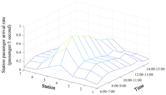
Figure 8.
Time-varying station passenger arrival rate.

Table 1.
Operation data setting.
Table 2.
Time-related parameter settings.
5.2. Optimization of Timetable During Trial Operation
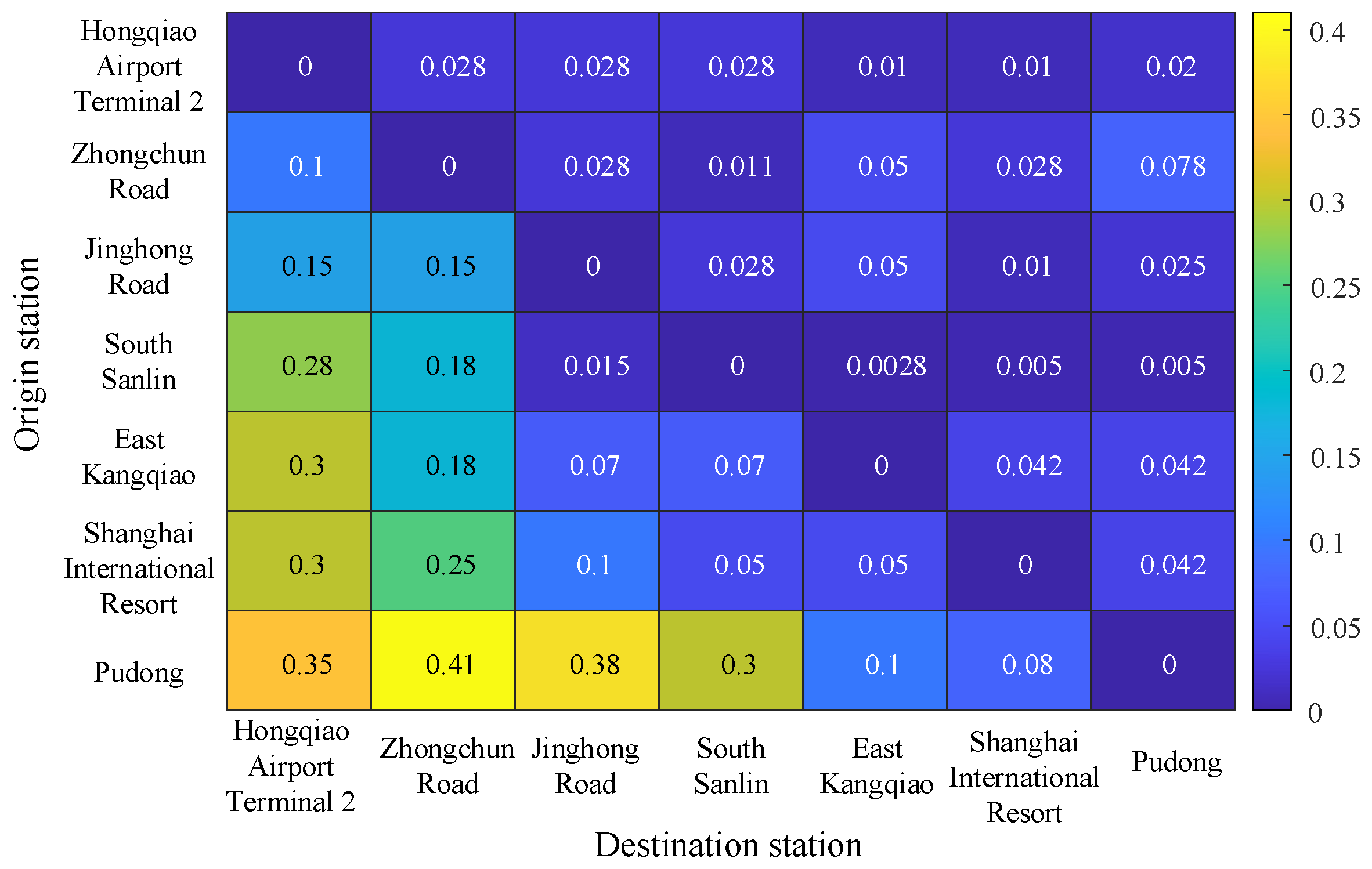
The Shanghai Suburban Railway airport link line is scheduled to initiate trial operations on 1 September 2024, and is expected to be officially operational by the end of 2024. The simulation in this section primarily focuses on optimizing the timetable during the trial operation phase. To demonstrate the validity and accuracy of the proposed model and method, the T-TPOS is compared with the TUOS-ELS. As can be seen from Figure 9, there is a large difference between the upstream and downstream passenger arrival rates, i.e., in Equation (14). This is a key factor in determining the number of trains running in both directions.
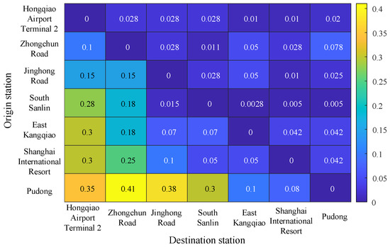
Figure 9.
OD passenger flow arrival rate.
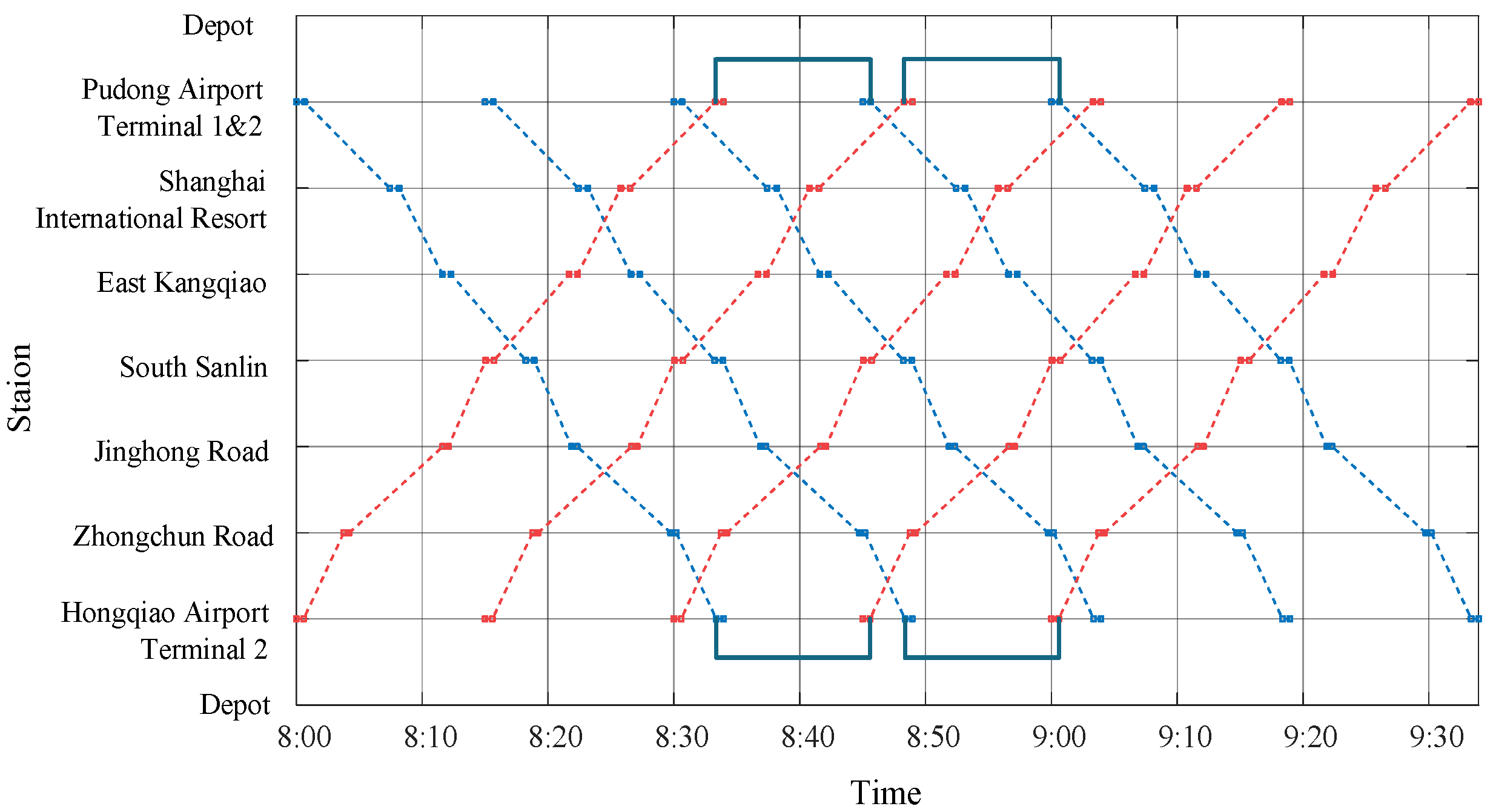
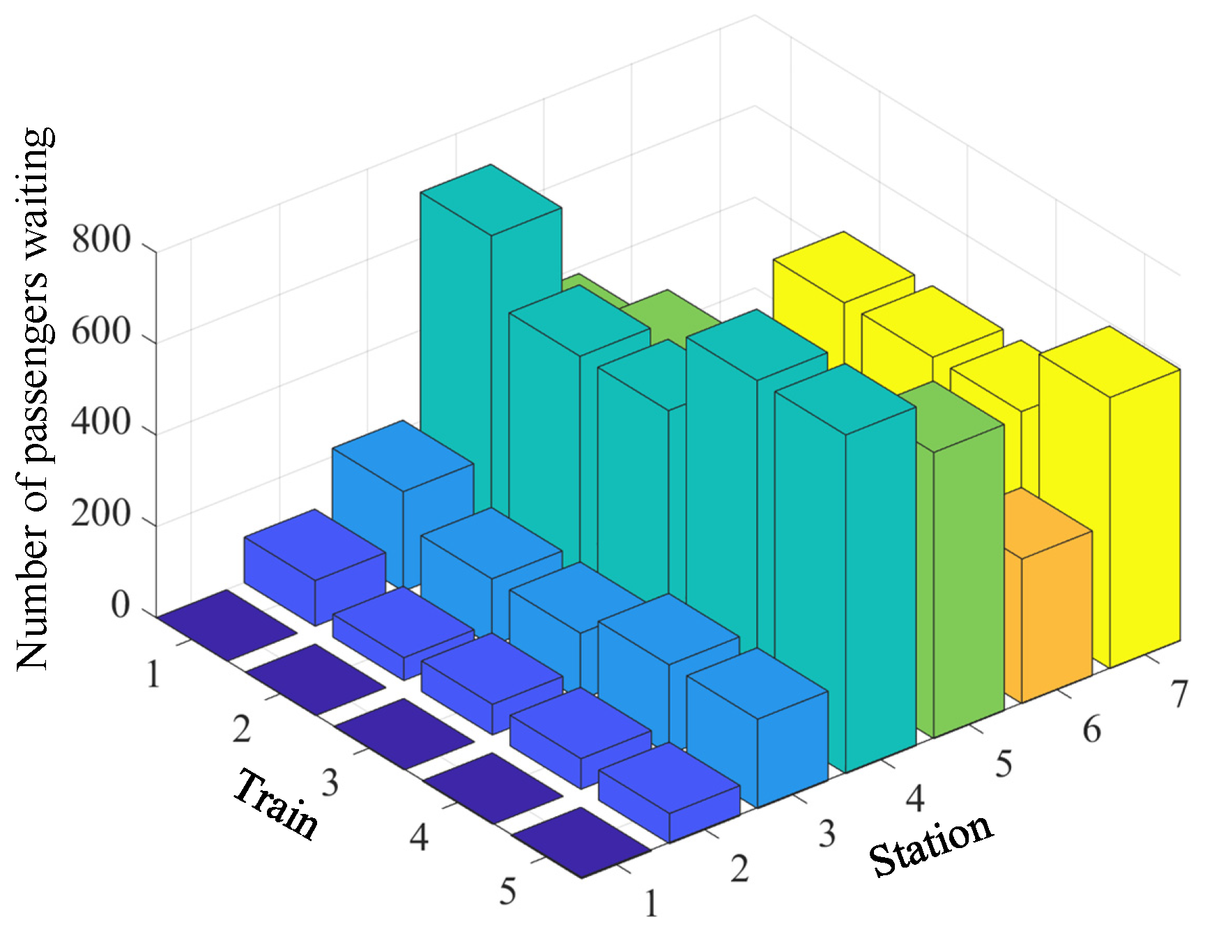
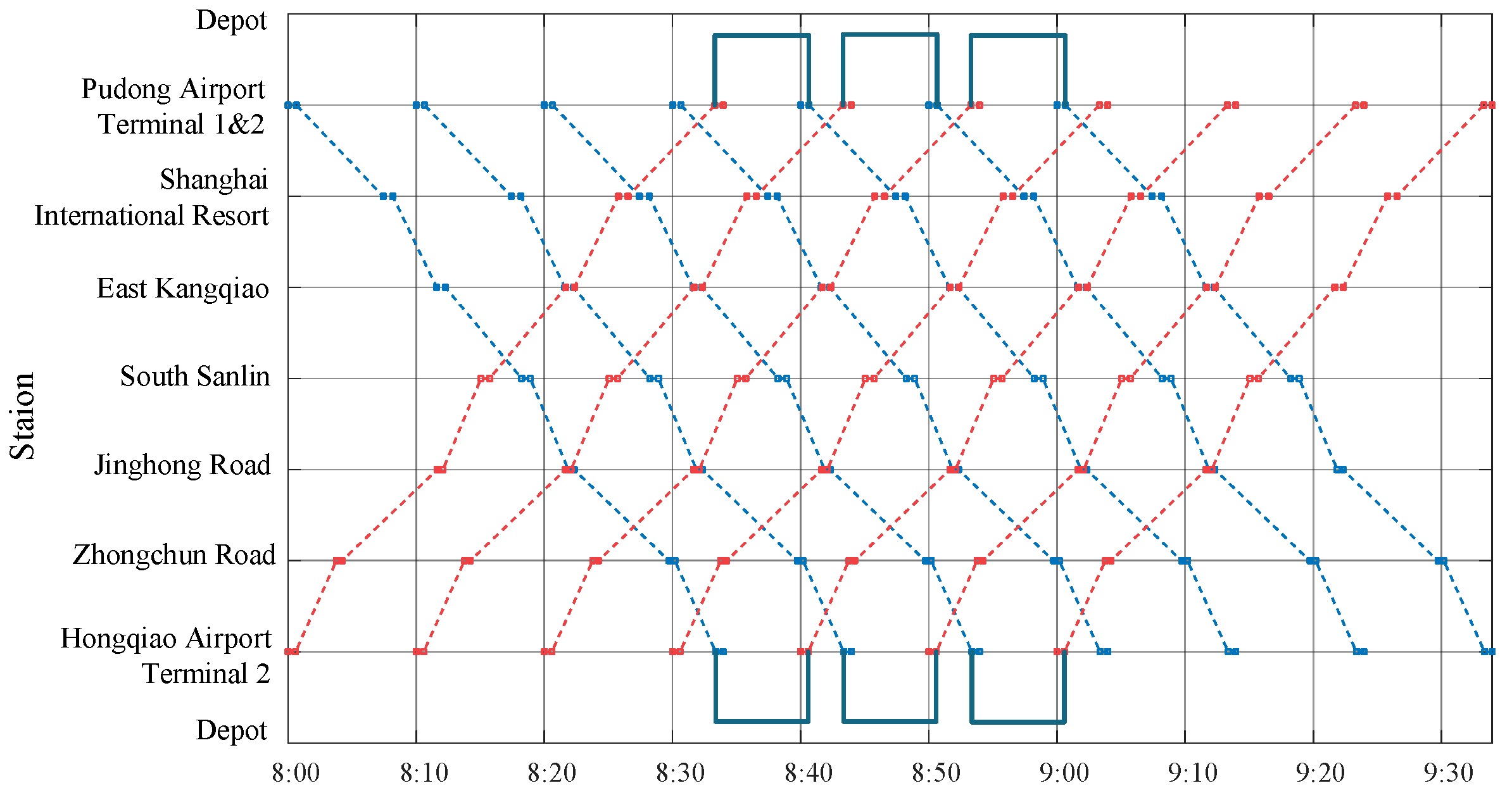
Based on the trial operation timetable of the Shanghai Suburban Railway airport link line, it is evident that the headway between trains is 15 min, and an all-stop behavior is adopted. Consequently, five trains operate in both the upstream and downstream directions. The timetable obtained by T-TPOS is shown in Figure 10. The number of passengers waiting on the stations is shown in Figure 11 and Figure 12. The train numbers in Figure 11 and Figure 12 are assigned based on the departure sequence of trains shown in Figure 10. For example, the train departing around 8:00 is assigned train number 1, while the train departing between 8:10 and 8:20 is assigned train number 2.
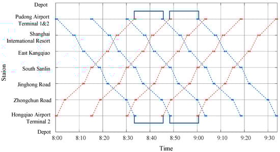
Figure 10.
The timetable of T-TPOS.

Figure 11.
Number of passengers waiting of upstream.
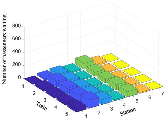
Figure 12.
Number of passengers waiting of downstream.
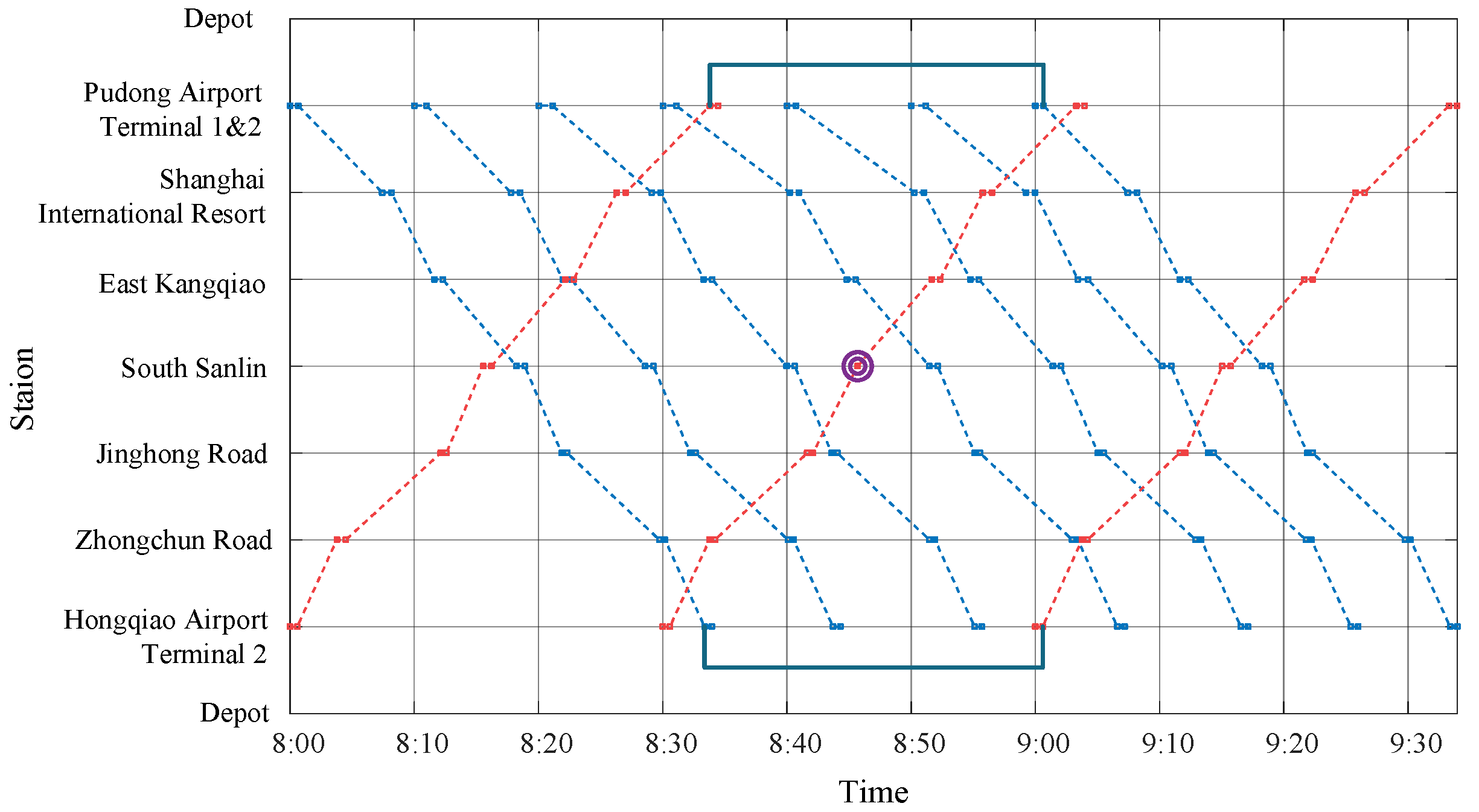
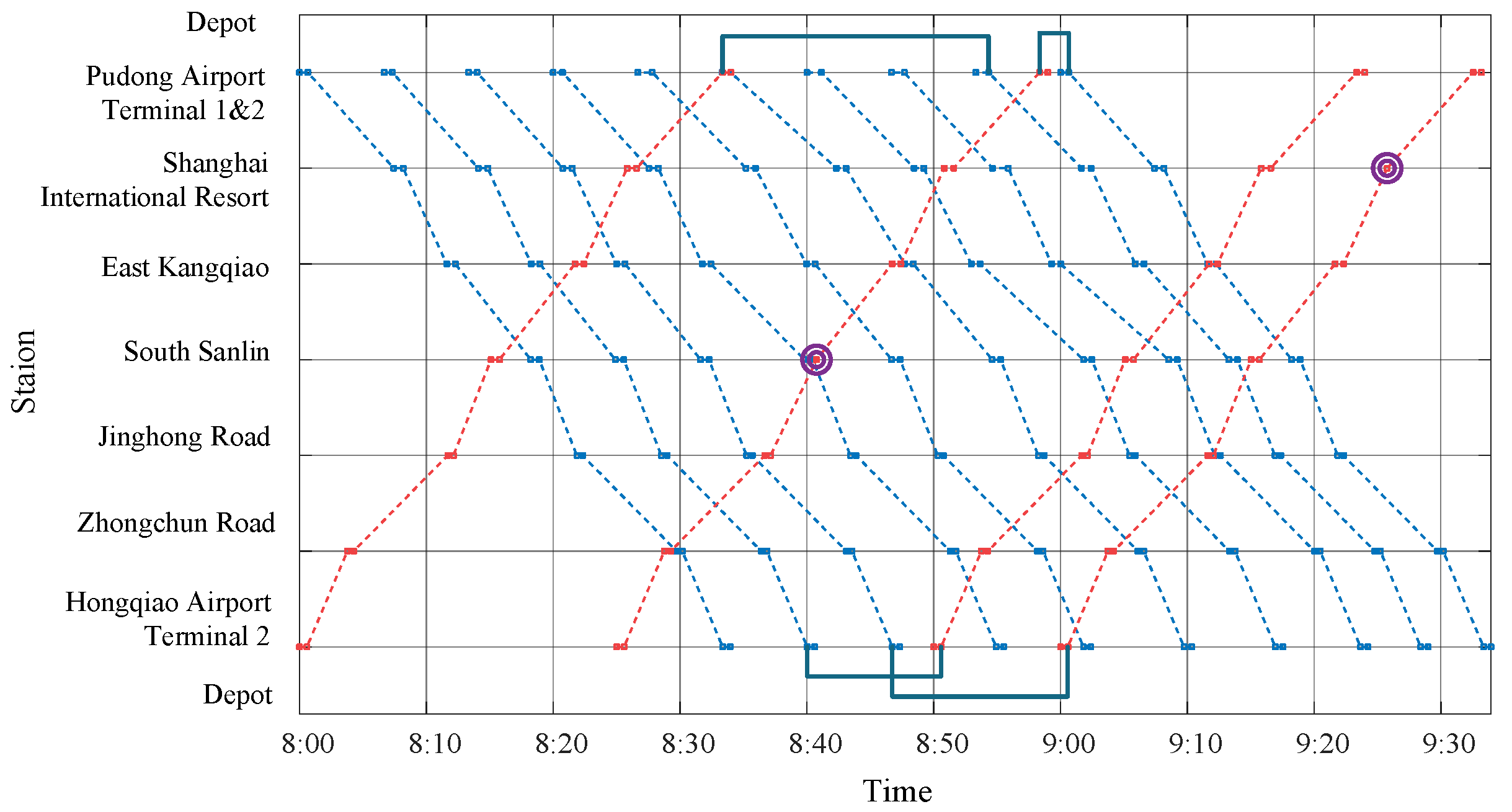
The optimized timetable of TUOS-ELS obtained by the GUROBI solver is shown in Figure 13. In Figure 13, the red dashed line and the blue dashed line indicate the time-station paths of trains in the downstream direction and the upstream direction, respectively. The double purple circles indicate the stations skipped by express trains in the downstream direction. Figure 14 and Figure 15 show the number of passengers waiting at each station in the upstream direction and downstream direction, respectively.
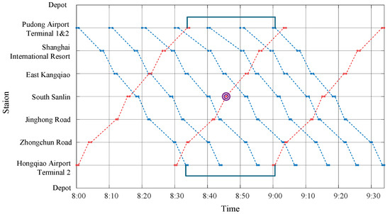
Figure 13.
The optimized timetable of TUOS-ELS.

Figure 14.
Number of passengers waiting in the upstream direction.
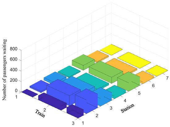
Figure 15.
Number of passengers waiting in the downstream direction.
The number of stops, the number of stranded passengers, and the total travel time of each train were counted for the two schemes, as shown in Table 3. Passengers’ total waiting time and on-board time are counted in Table 4. The value of objective function represents the total cost of the operator and the passenger in RMB, which is determined by setting the values of , i.e., . The term is derived from a simulation calculation, primarily including the energy consumption of train stopping, acceleration, deceleration, and equipment maintenance costs. Based on the fare range of 4–26 RMB for the Shanghai Suburban Railway airport link line, and considering the dissatisfaction of stranded passengers, is chosen as the middle value of the fare range, i.e., . For suburban trains running at 160 km/h, according to literature [6], it is known that the train consumes approximately 1 RMB per second, i.e., . Moreover, the values marked with * are used in the calculation of the objective function.
Table 3.
Comparison results including objective function values.
Table 4.
Comparison results including passengers’ total travel time.
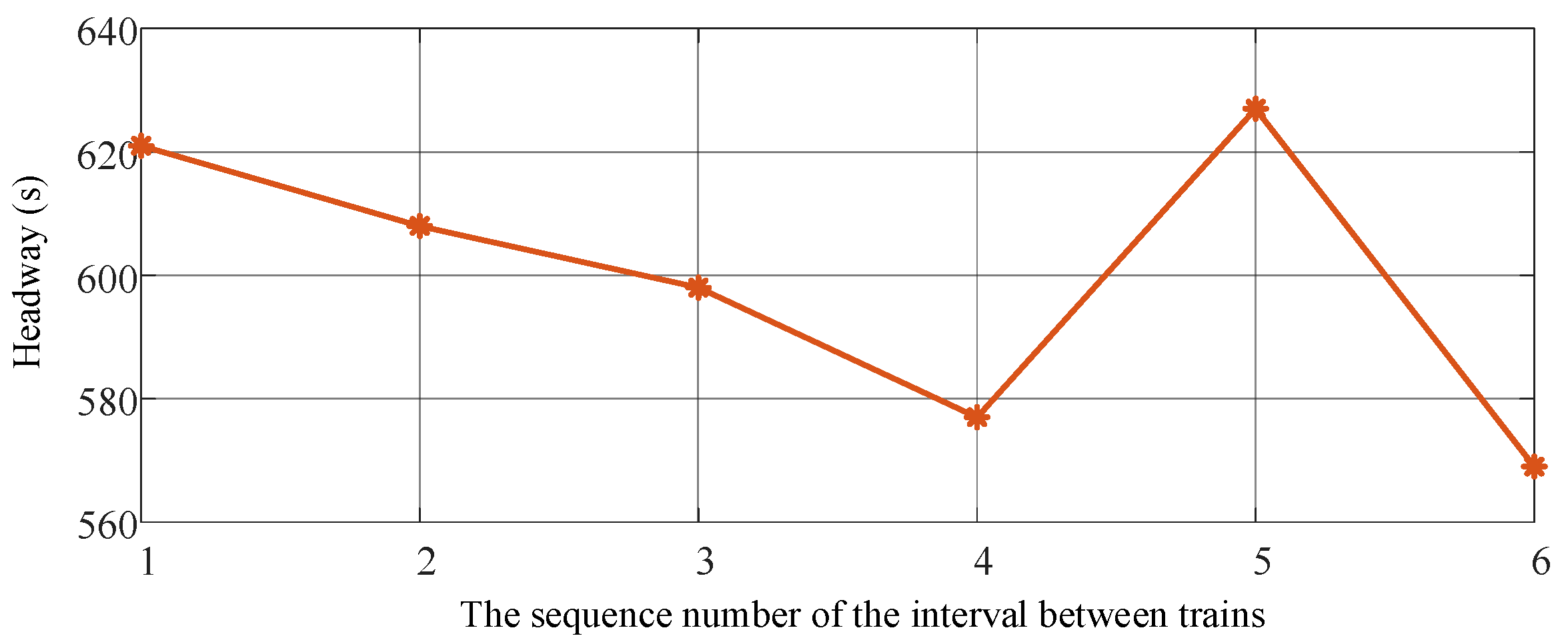
In Table 3, TUOS-ELS saves 38.59% in the total cost of the operator and the passenger compared to T-TPOS. The number of trains in the upstream direction was increased from 5 to 7, creating a shortened headway. The obtained headways for each train in the upstream direction are shown in Figure 16. All headways in the downstream direction are 1800 s. As a result, the number of stranded passengers decreased from 2489 to 196, and the total waiting time of passengers was greatly shortened from 2581.1 h to 1841.1 h in the upstream direction in Table 4. However, in the downstream, at the expense of a small number of stranded passengers, the reduction in the number of trains and the use of an express train (train 2) have significantly decreased the total travel time of trains from 10,185 s to 6139 s. Moreover, passengers’ on-board time were reduced by 8 h as compared with T-TPOS in the downstream direction.
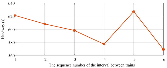
Figure 16.
Headway between trains.
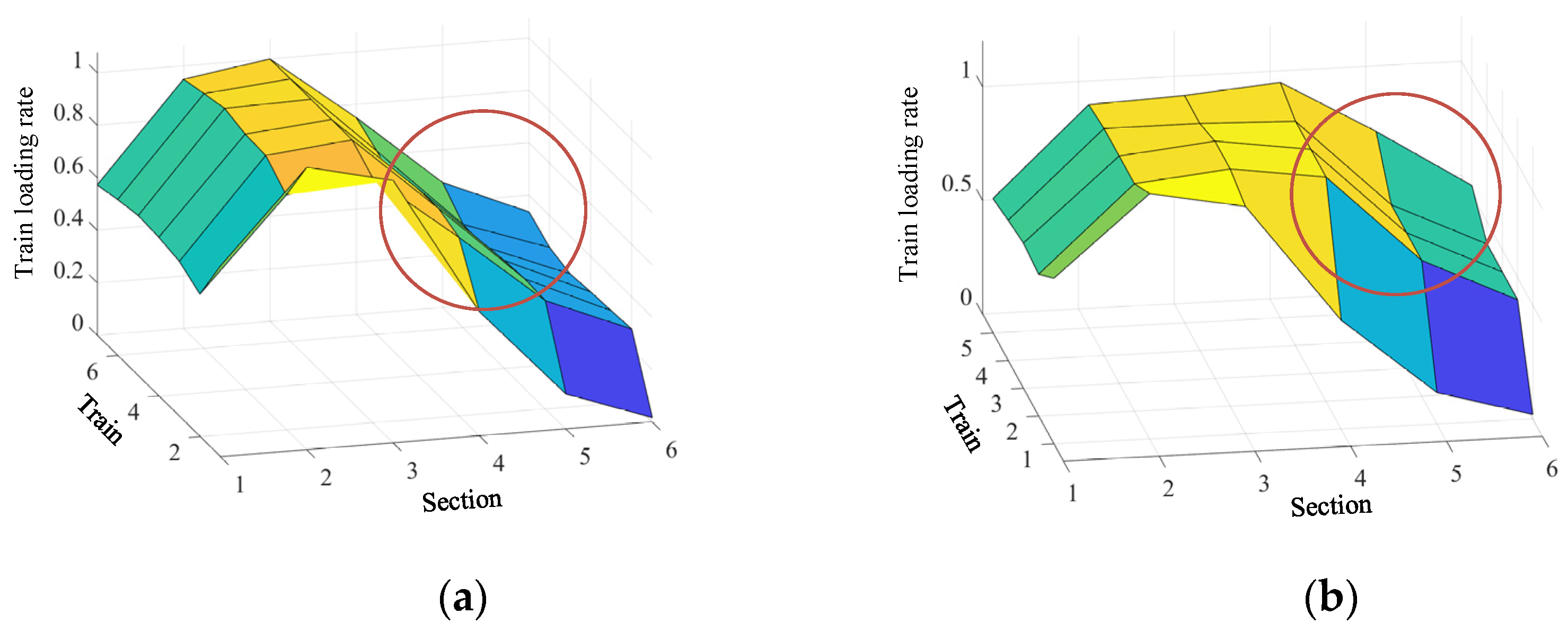
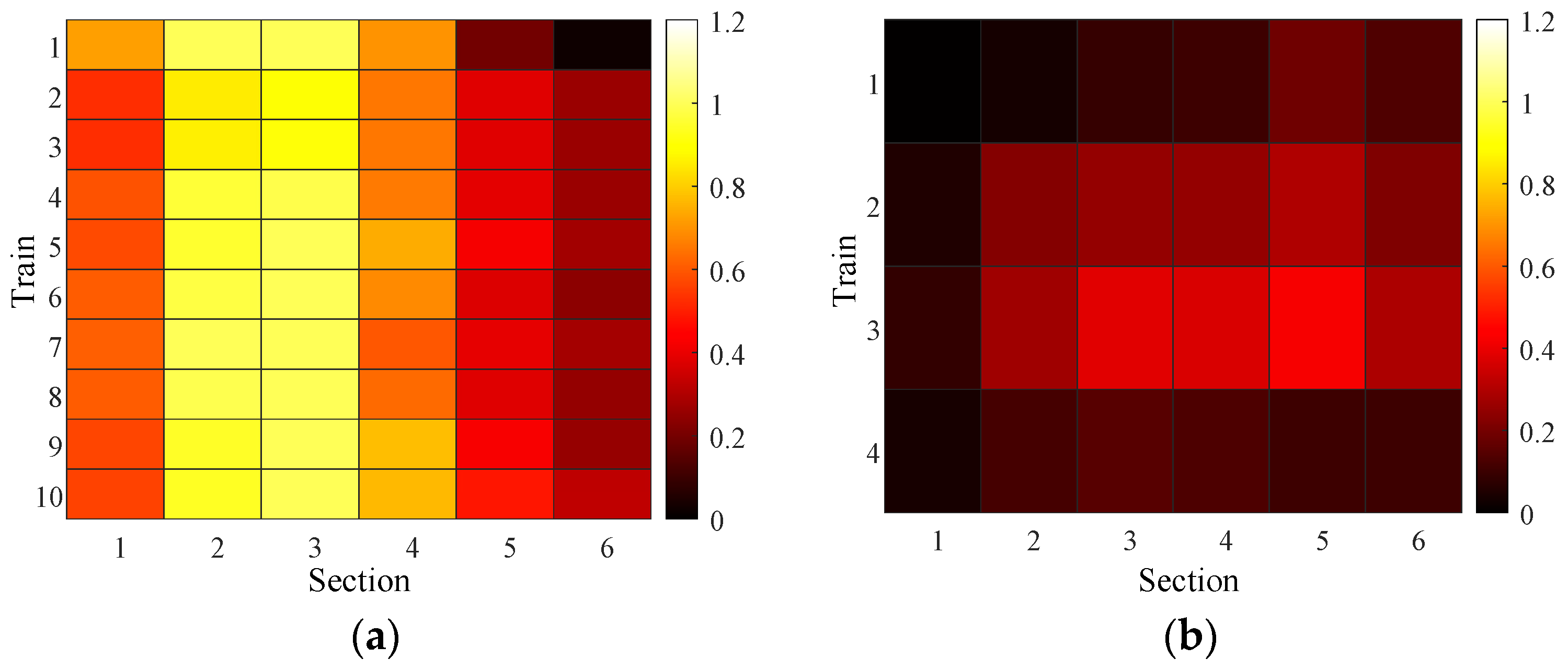
It is worth noting that TUOS-ELS can improve the trains’ loading rate in both directions. In Figure 17a,b, the maximum loading rates of TUOS-ELS and T-TPOS in the upstream direction are 107.64% and 107.82% respectively. Notably, the difference of maximum loading rates between the two schemes is not significant. But, Figure 17a,b illustrate that the trains loading rate under the TUOS-ELS rapidly decreases during the section from 3 to 6, whereas the trains loading rate under the T-TPOS remains consistently high. Meanwhile, in the downstream direction, the maximum loading rates under TUOS-ELS and T-TPOS are 39.27% and 20%. Figure 18a,b clearly demonstrates that the TUOS-ELS effectively enhances the trains’ loading rate and minimizes capacity waste.
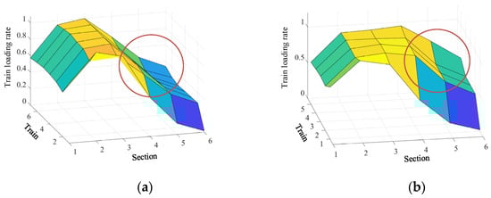
Figure 17.
Train loading rate in the upstream of TUOS-ELS and T-TPOS. (a) Train loading rate in the upstream of TUOS-ELS; (b) Train loading rate in the upstream of T-TPOS.
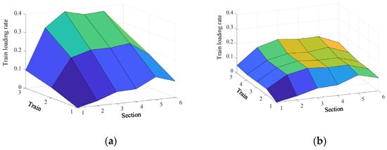
Figure 18.
Train loading rate in the downstream of TUOS-ELS and T-TPOS. (a) Train loading rate in the downstream of TUOS-ELS; (b) Train loading rate in the downstream of T-TPOS.
Based on the above analysis, compared to T-TPOS, the implementation advantages of TUOS-ELS can be reflected in both passenger service quality and operating costs. In terms of passenger service quality, TUOS-ELS can effectively reduce the total number of stranded passengers by 2202, the total passenger waiting time by 405.1 h, and the passenger on-board time in the downstream direction by 8 h. Additionally, TUOS-ELS can improve trains’ load rate, thereby alleviating passenger congestion. From an operational cost perspective, reducing the total number of train stops can minimize the traction and braking processes, which helps lower energy consumption and equipment maintenance.
5.3. Optimization of Timetable to Address Varying Passenger Demands
After the start of official operation of the Shanghai Suburban Railway airport link line, there is likely to be an increase in passenger demand. To further illustrate the generality of the proposed solution and model, this section examines the timetable optimization to address varying passenger demand. Based on the OD passenger arrival rate shown in Figure 9, when is doubled, such as to and , it is possible to study the timetable of TUOS-ELS during the official operation period.
When the OD passenger arrival rate is in the official operation period, the optimization result indicates that ten trains should operate in the upstream direction, while four trains should run in the downstream direction. The optimized timetable of TUOS-ELS is shown in Figure 19. The optimized results using the TUOS-ELS are compared with those obtained from the T-TPOS (Figure 20), as shown in Table 5 and Table 6. The operator’s and passenger’s travel costs are reduced by 35.28% after optimization, and shows that the multi-strategy combination method still maintains a stable optimization effect in scenarios of increased numbers of traveling passengers.
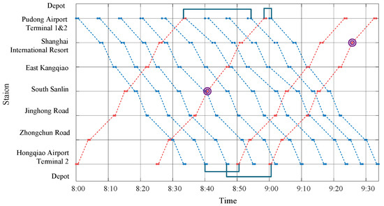
Figure 19.
The optimized timetable of TUOS-ELS.
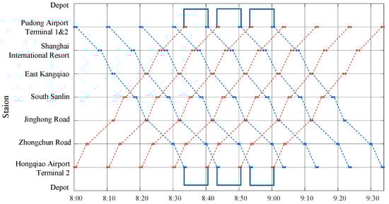
Figure 20.
The optimized timetable of T-TPOS.
Table 5.
Comparison results including objective function values.
Table 6.
Comparison results including passengers’ total travel time.
Note: Values marked with * are used as calculated objective value.
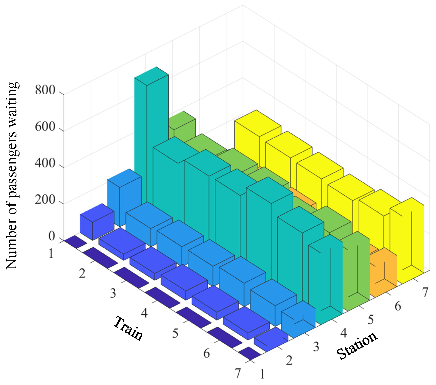
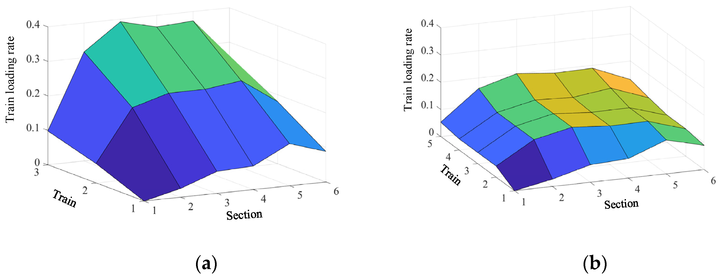
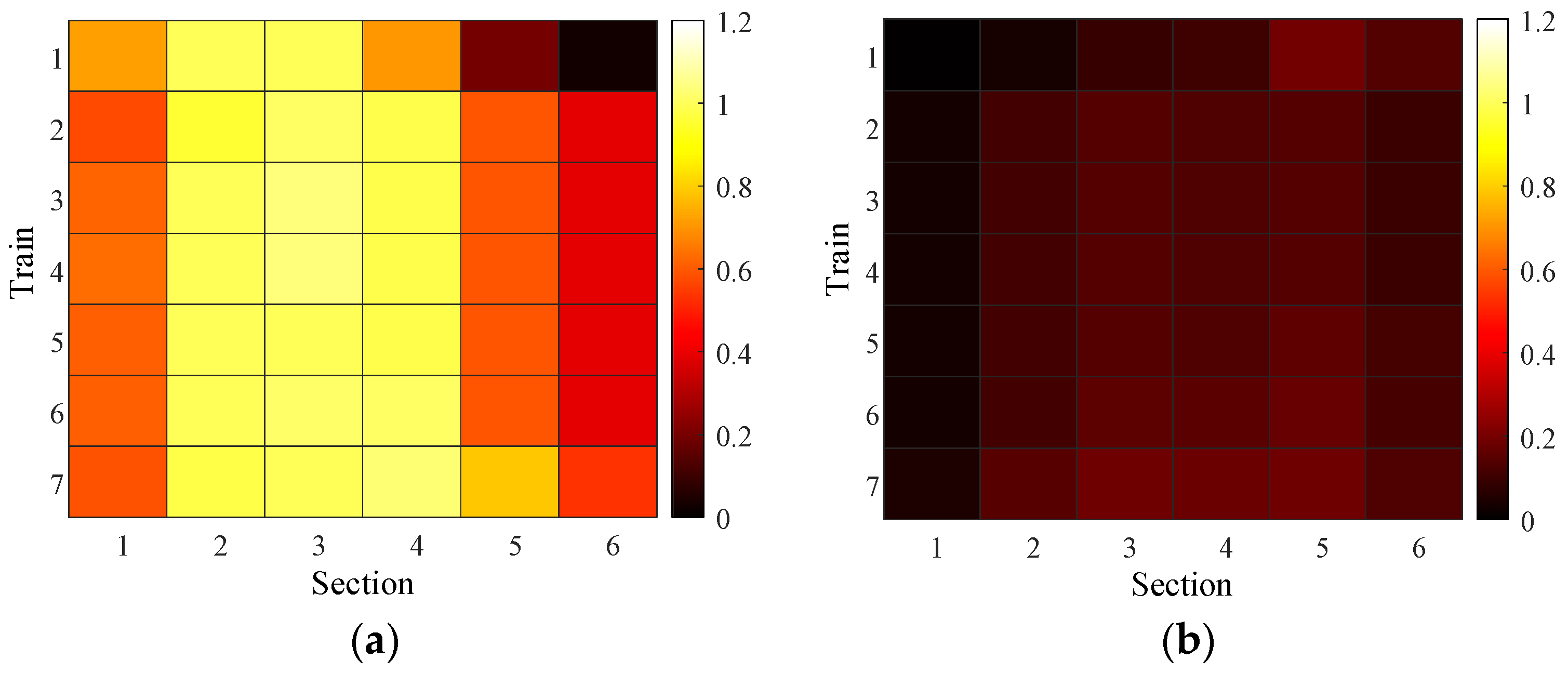
To illustrate the trains’ loading rate in more detail, per-train loading rate heat maps are presented in Figure 21 and Figure 22. The total number of passengers waiting in the upstream direction for both TUOS-ELS and T-TPOS is 14,910. Meanwhile, the total number of passengers waiting in the downstream direction for both is 2280. From these two figures, it can be clearly seen that the brighter and yellower the color is, the higher the train loading rate is. The rate is close to 1.2, i.e., 120%. This reflects more crowding of passengers inside the carriages. Figure 21a and Figure 22a show the trains’ loading rates in the upstream direction for both TUOS-ELS and T-TPOS; the average loading rates were 64.33% and 75.54%, respectively. In the upstream direction, as the number of trains increased and headways shortened under TUOS-ELS, the loading rate notably declined, beginning with train 2 in Section 4, Section 5 and Section 6. The degree of passenger crowding was effectively alleviated. Figure 21b and Figure 22b indicate that trains operating in the downstream direction suffered from the problem of loading fewer passengers; their average loading rates were 18.54% and 12.03%, respectively. In the TUOS-ELS, loading rates of between 30% and 50% are achieved by train 2 and train 3 in Section 2, Section 3, Section 4, Section 5 and Section 6. The loading rate of all trains in all sections is less than 20% under T-TPOS, which is a strong indication that TUOS-ELS is effective in improving the trains’ loading rates and increasing the use of train resources.
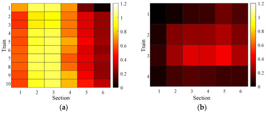
Figure 21.
Heat maps of train loading rate under TUOS-ELS. (a) Heat maps of train loading rate in the upstream of TUOS-ELS; (b) Heat maps of train loading rate in the downstream of TUOS-ELS.
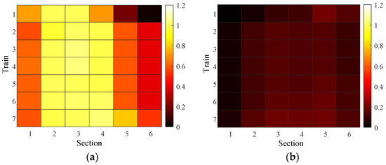
Figure 22.
Heat maps of train loading rate under T-TPOS. (a) Heat maps of train loading rate in the upstream of T-TPOS; (b) Heat maps of train loading rate in the downstream of T-TPOS.
Similar to the results of the previous trial operation phase, TUOS-ELS still shows significant advantages over T-TPOS in terms of improving passenger service quality and reducing operational costs. TUOS-ELS reduced the number of stranded passengers by 3013, total passenger waiting time by 327.5 h, and the total number of stops by two. It also decreased the average loading rate in the upstream direction by 11.21% and increased the average loading rate of the downstream direction by 5.61%.
In summary, the optimization model and the multi-strategy method demonstrate versatility, effectively addressing lower passenger demand (with larger headways) and higher passenger demand (with smaller headways). In particular, the use of an unpaired operation strategy can flexibly improve the allocation of train capacity. While the implementation of express/local trains can shorten travel time, it also facilitates the allocation of capacity to required stations through skip-stopping behavior. Although two case analyses were conducted using the Shanghai Suburban Railway, the TUOS-ELS, the MILP model established, and the optimization procedure designed in this paper are all applicable to urban rail transit lines that exhibit the tidal passenger flow phenomenon, such as metro lines, suburban rail lines, and tram lines.
6. Conclusions
This paper presents a multi-strategy timetable optimization method of use in addressing the tidal passenger flow phenomenon, which is the TUOS-ELS. Specifically, a TUOS-ELS including an unpaired operation strategy and an express/local train operation strategy is proposed. TUOS-ELS has the flexibility to solve the problem of the uneven distribution of passenger flow in both directions compared to the traditional train paired operation strategy (T-TPOS). Timetables are optimized during the morning rush hour for the trial and official operation period (i.e., increased passenger flow) of the Shanghai Suburban Railway airport link line. With the objective of reducing the number of stranded passengers, the number of stops, and the total trains’ travel time, the objective values of 38.59% and 35.28% were reduced during the trial and official operation period, respectively. From the perspective of the trains’ loading rate, adopting the TUOS-ELS can improve the crowding of the carriages in the direction of heavy passenger flow and can increase the resource utilization in the other direction. Overall, the multi-strategy optimization method proposed in this paper effectively reduces operator costs and improves passenger service quality. It is worth noting that TUOS-ELS is a method suitable for long-distance rail transit and uneven passenger flow distribution. Its effectiveness benefits are minimal for short-distance or scenarios with even passenger flow. Considering the performance of the model solution time, as the number of trains and stations increases, the solution time also increases. But, for a study period of hours, the GUROBI solver can always obtain an accurate solution in an acceptable time.
In summary, this study expands the theoretical framework of the field of train operation optimization, proposing the idea of improving passenger service quality and reducing operational costs through a multi-strategy method. Moreover, this method has the advantage of being simple and feasible at the transportation organization level, helping railway operators achieve optimized resource allocation. In future research, flexible groupings can be developed based on this study to further improve the matching of train capacity and passenger flow and be applied to more passenger flow scenarios.
Author Contributions
Conceptualization, B.Y. and P.S.; methodology, B.Y.; software, W.J.; validation, W.J., B.Y. and P.S.; formal analysis, R.D.; investigation, W.J.; resources, B.Y.; data curation, B.Y.; writing—original draft preparation, W.J.; writing—review and editing, P.S.; visualization, R.D.; supervision, P.S.; project administration, B.Y.; funding acquisition, P.S. All authors have read and agreed to the published version of the manuscript.
Funding
This research was funded by the project of CRRC Changchun Railway Vehicles Co., Ltd., project number 2023CCB171.
Institutional Review Board Statement
Not applicable.
Informed Consent Statement
Not applicable.
Data Availability Statement
The original contributions presented in the study are included in the article. Further inquiries can be directed to the corresponding author.
Acknowledgments
The authors would like to express their sincere thanks to all of the editors and reviewers.
Conflicts of Interest
Author Wenbin Jin was employed by the company CRRC Changchun Railway Vehicles Co., Ltd. The authors declare that this study received funding from CRRC Changchun Railway Vehicles Co., Ltd. The funder was not involved in the study design, collection, analysis, interpretation of data, the writing of this article or the decision to submit it for publication.
References
- Tang, L.; Zhao, Y.; Cabrera, J.; Ma, J.; Tsui, L. Forecasting Short-Term Passenger Flow: An Empirical Study on Shenzhen Metro. IEEE Trans. Intell. Transp. Syst. 2019, 20, 3613–3622. [Google Scholar] [CrossRef]
- Yin, J.; Yang, L.; Tang, T.; Gao, Z.; Ran, B. Dynamic passenger demand oriented metro train scheduling with energy-efficiency and waiting time minimization: Mixed-integer linear programming approaches. Transp. Res. B-Meth. 2017, 97, 182–213. [Google Scholar] [CrossRef]
- Zhuo, S.; Miao, J.; Meng, L.; Yang, L.; Shang, P. Demand-driven integrated train timetabling and rolling stock scheduling on urban rail transit line. Transp. A 2024, 20, 2181024. [Google Scholar] [CrossRef]
- Chen, Z.; Li, X.; Zhou, X. Operational design for shuttle systems with modular vehicles under oversaturated traffic: Continuous modeling method. Transp. Res. B-Meth. 2020, 132, 76–100. [Google Scholar] [CrossRef]
- Sun, L.; Jin, J.; Lee, D.; Axhausen, K.; Erath, A. Demand-driven timetable design for metro services. Transp. Res. Part C Emerg. Technol. 2014, 46, 284–299. [Google Scholar] [CrossRef]
- Li, S.; Xu, R.; Han, K. Demand-oriented train services optimization for a congested urban rail line: Integrating short turning and heterogeneous headways. Transp. A 2019, 15, 1459–1486. [Google Scholar] [CrossRef]
- Yang, L.; Qi, J.; Li, S.; Gao, Y. Collaborative optimization for train scheduling and train stop planning on high-speed railways. Omega 2016, 64, 57–76. [Google Scholar] [CrossRef]
- Xu, X.; Li, C.L.; Xu, Z. Train timetabling with stop-skipping, passenger flow, and platform choice considerations. Transp. Res. B-Meth. 2021, 150, 52–74. [Google Scholar] [CrossRef]
- Zhang, F.; Li, S.; Yuan, Y.; Zhang, J.; Yang, L. Approximate dynamic programming approach to efficient metro train timetabling and passenger flow control strategy with stop-skipping. Eng. Appl. Artif. Intell. 2024, 127, 107393. [Google Scholar] [CrossRef]
- Yuan, Y.; Li, S.; Liu, R. Decomposition and approximate dynamic programming approach to optimization of train timetable and skip-stop plan for metro networks. Transp. Res. Part C Emerg. Technol. 2023, 157, 104393. [Google Scholar] [CrossRef]
- Rodolphe, Farrando; Farhi, N.; Christoforou, Z.; Urban, A. A mathematical model for a two-service skip-stop policy with demand-dependent dwell times. J. Rail Transp. Plan. Manag. 2024, 31, 100461.
- Liu, Z.; Pan, J.; Yang, Y.; Chi, X. An energy-efficient timetable optimization method for express/local train with on-board passenger number considered. IEEE Trans. Intell. Transp. Syst. 2024, 18, 2068–2088. [Google Scholar] [CrossRef]
- Zhang, R.; Yin, S.; Ye, M.; Yang, Z.; He, S. A Timetable Optimization Model for Urban Rail Transit with Express/Local Mode. J. Adv. Transport. 2021, 2021, 5589185. [Google Scholar] [CrossRef]
- Jin, B.; Guo, Y.; Wang, Q. Integrated scheduling method of timetable and rolling stock assignment scheme considering long and short routing. China Railw. Sci. 2022, 43, 173–181. [Google Scholar]
- Blanco, V.; Conde, E.; Hinojosa, Y.; Puerto, J. An optimization model for line planning and timetabling in automated urban metro subway networks. A case study. Omega 2020, 92, 102165. [Google Scholar] [CrossRef]
- Sun, P.; Yao, B.; Wang, Q.; Chen, S.; Lin, X.; Huang, Z. Optimization of unpaired timetable with express/local mode for the phenomenon of tidal passenger flow. In Proceedings of the IEEE 10th International Power Electronics and Motion Control Conference, Chengdu, China, 17–20 May 2024. [Google Scholar]
- Shi, J.; Yang, J.; Yang, L.; Tao, L. Safety-oriented train timetabling and stop planning with time-varying and elastic demand on overcrowded commuter metro lines. Transp. Res. E-Log. 2023, 175, 103136. [Google Scholar] [CrossRef]
- Zhou, H.; Qi, J.; Yang, L.; Shi, J.; Pan, H.; Gao, Y. Joint optimization of train timetabling and rolling stock circulation planning: A novel flexible train composition mode. Transp. Res. B-Meth 2022, 162, 352–385. [Google Scholar] [CrossRef]
- Zhao, S.; Yang, H.; Wu, Y. An integrated approach of train scheduling and rolling stock circulation with skip-stopping pattern for urban rail transit lines. Transp. Res. Part C Emerg. Technol. 2021, 128, 103170. [Google Scholar] [CrossRef]
- Cao, Z.; Ceder, A.; Li, D.; Zhang, S. Robust and optimized urban rail timetabling using a marshaling plan and skip-stop operation. Transp. A 2020, 16, 1217–1249. [Google Scholar] [CrossRef]
- Lusby, R.M.; Larsen, J.; Bull, S. A survey on robustness in railway planning. Eur. J. Oper. Res. 2018, 266, 1–15. [Google Scholar] [CrossRef]
- Mo, P.; Yang, L.; D’Ariano, A. Energy-Efficient Train Scheduling and Rolling Stock Circulation Planning in a Metro Line: A Linear Programming Approach. IEEE Trans. Intell. Transp. Syst. 2021, 21, 3621–3633. [Google Scholar] [CrossRef]
- Tang, L.; Xu, X. Optimization for operation scheme of express and local trains in suburban rail transit lines based on station classification and bi-level programming. J. Rail. Transport. Plan. 2022, 21, 100283. [Google Scholar] [CrossRef]
- Bucak, S.; Demirel, T. Train timetabling for a double-track urban rail transit line under dynamic passenger demand. Comput. Ind. Eng. 2022, 163, 107858. [Google Scholar] [CrossRef]
- Qi, J.; Li, S.; Gao, Y.; Yang, K.; Liu, P. Joint optimization model for train scheduling and train stop planning with passengers distribution on railway corridors. J. Oper. Res. Soc. 2018, 69, 556–570. [Google Scholar] [CrossRef]
- Cacchiani, V.; Qi, J.; Yang, L. Robust optimization models for integrated train stop planning and timetabling with passenger demand uncertainty. Transp. Res. B-Meth. 2020, 136, 1–29. [Google Scholar] [CrossRef]
- Högdahl, J.; Bohlin, M. A combined simulation-optimization approach for robust timetabling on main railway lines. Transp. Sci. 2023, 57, 52–81. [Google Scholar] [CrossRef]
- Gao, Y.; Kroon, L.; Schmidt, M.; Yang, L. Rescheduling a metro line in an over-crowded situation after disruptions. Transp. Res. B-Meth. 2016, 93, 425–449. [Google Scholar] [CrossRef]


Disclaimer/Publisher’s Note: The statements, opinions and data contained in all publications are solely those of the individual author(s) and contributor(s) and not of MDPI and/or the editor(s). MDPI and/or the editor(s) disclaim responsibility for any injury to people or property resulting from any ideas, methods, instructions or products referred to in the content. |
© 2024 by the authors. Licensee MDPI, Basel, Switzerland. This article is an open access article distributed under the terms and conditions of the Creative Commons Attribution (CC BY) license (https://creativecommons.org/licenses/by/4.0/).