A Comprehensive Review on Uncertainty and Risk Modeling Techniques and Their Applications in Power Systems

Abstract

The increasing integration of renewable energy sources (RESs) into power systems has introduced new complexities due to the inherent variability and uncertainty of these energy sources. In addition to the uncertainty in RES generation, the demand-side load of power systems is also subject to fluctuations, further complicating system operations. Addressing these challenges requires effective modeling and assessment techniques to quantify and mitigate the risks associated with system uncertainties. This paper evaluates the impact of various uncertainty modeling techniques on power system reliability with wind farm integration. Furthermore, this paper reviews the state of the art of the various uncertainty and risk modeling techniques in power systems. Through a detailed case study, the performance of these techniques in modeling uncertainties of wind speeds is analyzed. Based on the results, the integration of wind turbines improves the system’s overall reliability when there is a reduction in conventional power plants (CPPs)’ generation, which are dispatchable energy sources providing a stable and flexible supply. However, the generation of wind farms is associated with uncertainty. The results show Monte Carlo simulation combined with the K-Means method is consistently a more accurate uncertainty model for wind speeds, closely aligning with real-case scenarios, compared to other methods such as Markov Chain Monte Carlo (MCMC), robust optimization (RO), and information-gap decision theory (IGDT).

1. Introduction

The increasing integration of renewable energy sources (RESs), particularly wind farms, introduces significant uncertainties into power systems. These uncertainties, combined with variability in both generation and demand, complicate system operations and create challenges in maintaining reliability. Effective decision-making under uncertainty is crucial for ensuring the reliable and resilient operation of power systems. This paper reviews the state-of-the-art techniques for modeling uncertainty and risk in power systems, emphasizing their vital role in managing the challenges posed by uncertain power generation and demand. The goal is to bridge theoretical advancements with practical applications to enhance the robustness of power systems. As modern power systems evolve with the growing adoption of RESs, the need for sophisticated risk management techniques becomes more critical. These methods have advanced significantly, transitioning from basic statistical tools to complex computational models designed to address dynamic system uncertainties. This evolution reflects broader developments in our understanding of risk, driven by innovations in mathematics, statistics, and computational science. The paper traces the progression of risk theories, from classical probability models to contemporary approaches tailored for the uncertainties introduced by renewable energy integration. The review covers how these risk modeling techniques have been applied across energy systems, highlighting their adaptability to new challenges. Special attention is given to the role of probabilistic models in scenarios with incomplete information, which are central to predicting outcomes and assessing risks in complex systems. Additionally, possibilistic frameworks, such as fuzzy logic and Dempster–Shafer theory, are explored for their ability to handle imprecise data, offering flexibility in systems with significant uncertainty or data scarcity. Further, the paper evaluates key analytical techniques such as Monte Carlo simulation, Latin Hypercube Sampling, and point estimation methods (PEMs). These are assessed for their effectiveness in different contexts, including environmental risk management and power system optimization. Case studies demonstrate their practical application and highlight where each method offers the most value. Advanced methodologies, such as robust optimization (RO) and information-gap decision theory (IGDT), are also examined for their growing importance in managing uncertainty in the energy and finance sectors. By integrating a range of methodologies, probabilistic, possibilistic, and decision theory-based, the paper advocates for a holistic, cross-disciplinary approach to risk management. This integrated perspective not only strengthens theoretical models but also ensures their applicability in real-world power system operations. The paper concludes by discussing the policy and regulatory implications of these models, emphasizing the need for ongoing research and collaboration to refine risk management strategies. Ultimately, this review aims to equip practitioners and policymakers with the tools and knowledge to develop power systems that are not only resilient and reliable but also adaptable to the uncertainties inherent in modern energy landscapes.

The early interest in applying probability methods to evaluate generating capacity requirements emerged in 1933 [1]. A pivotal moment occurred at the American Institute of Electrical Engineers conference in 1947, where the application of probability theory to account for generation unit reliability was introduced. Throughout the 1950s and into the 1960s, the concept of the loss of load probability (LOLP) was further expanded. Notable contributions from engineers like G. Calabrese and C.W. Watchorn helped establish a consensus on acceptable reliability criteria. The LOLP is the probability that a power system will experience a shortage in generation capacity relative to demand, potentially leading to involuntary load shedding. It measures the likelihood of an energy deficit over a specified period. The LOLP refers to a probability of outages, where the loss of load expectation (LOLE) describes an expected value. The LOLE represents the expectation that available generation capacity will be inadequate to supply customers’ demand at a given period. Renewable power plants and energy islands play a paramount role in electricity generation due to the transition to green and sustainable energies. The uncertain and intermittent nature of these systems makes the power system reliability assessment more complicated. Monte Carlo simulation, Bayesian Networks, and State Enumeration methods are widely used techniques for modeling uncertainty in power systems, particularly as the integration of RESs adds significant variability. Monte Carlo simulation generates numerous random scenarios based on uncertain variables, such as load demand and renewable generation, enabling system operators to evaluate probabilistic outcomes and assess risks like generation shortfalls or equipment failures. Bayesian Networks provide a probabilistic graphical approach that models the dependencies between system components and allows operators to update risk assessments dynamically as new information becomes available, making them especially useful for real-time decision-making. State Enumeration, on the other hand, systematically evaluates all possible system states under uncertainty, often in a reduced or aggregated form, to identify the worst-case scenarios or critical system vulnerabilities. These methods help ensure robust decision-making in the face of uncertainties in both power generation and system demand, enabling more reliable and resilient grid operations. Risk modeling in safety science is evolving to address complex challenges like hybrid threats, emphasizing private sector roles in resilience and the importance of geopolitical awareness [2]. The precautionary principle, often criticized, is reframed as a valuable tool for managing significant uncertainties when integrated with scientific decision-making [3]. Additionally, systems thinking, such as the iceberg model, supports a shift from reactive to proactive safety strategies, promoting sustainable risk management [4]. These approaches collectively advance the field toward holistic and anticipatory frameworks.

This paper aims to provide a comprehensive evaluation of uncertainty and risk modeling techniques in power systems, focusing on their applications and implications in renewable energy integration. To complement this theoretical review, we include a detailed case study that demonstrates the practical distinctions between various methods. The inclusion of the case study serves the following purposes:

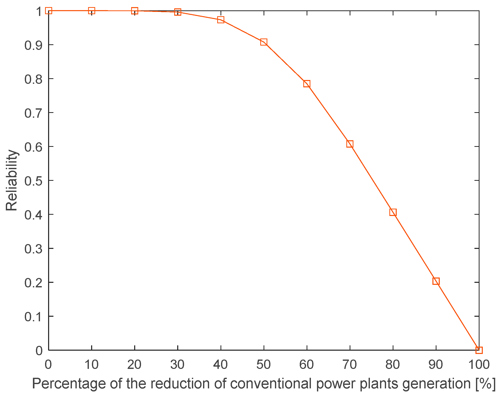
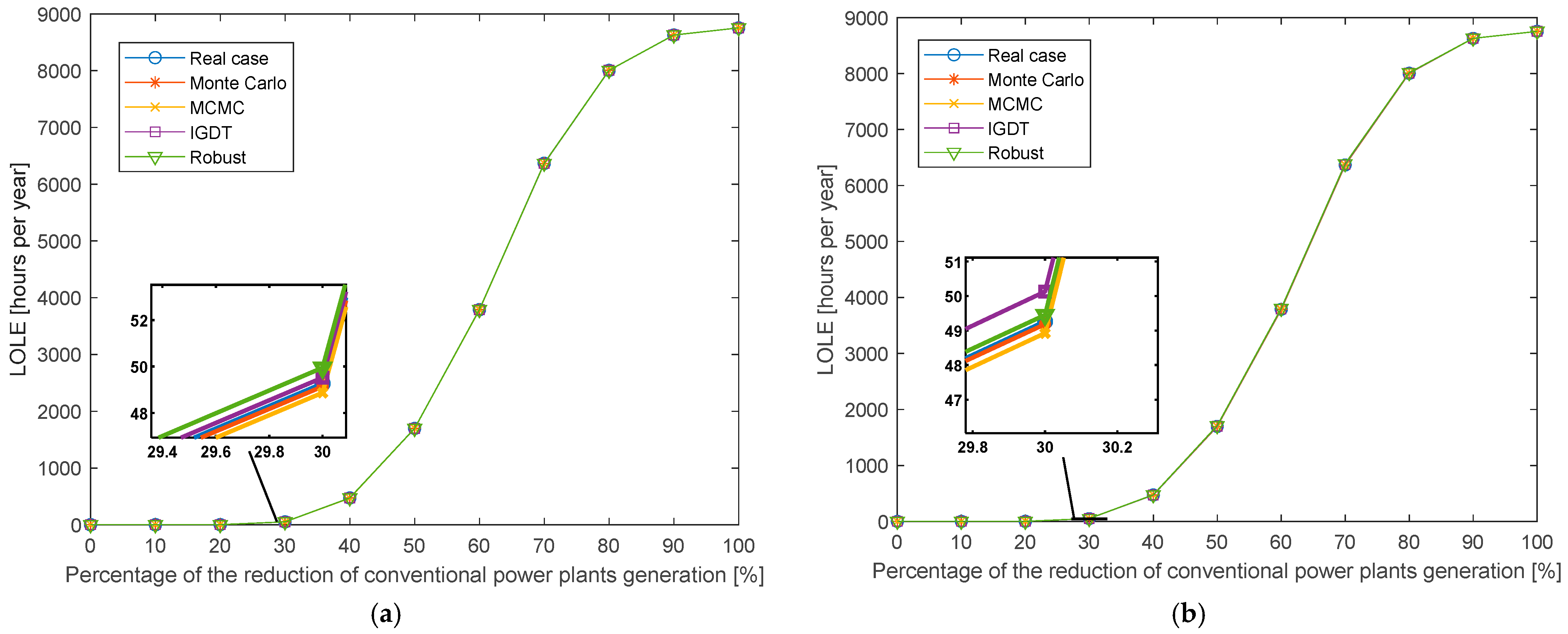
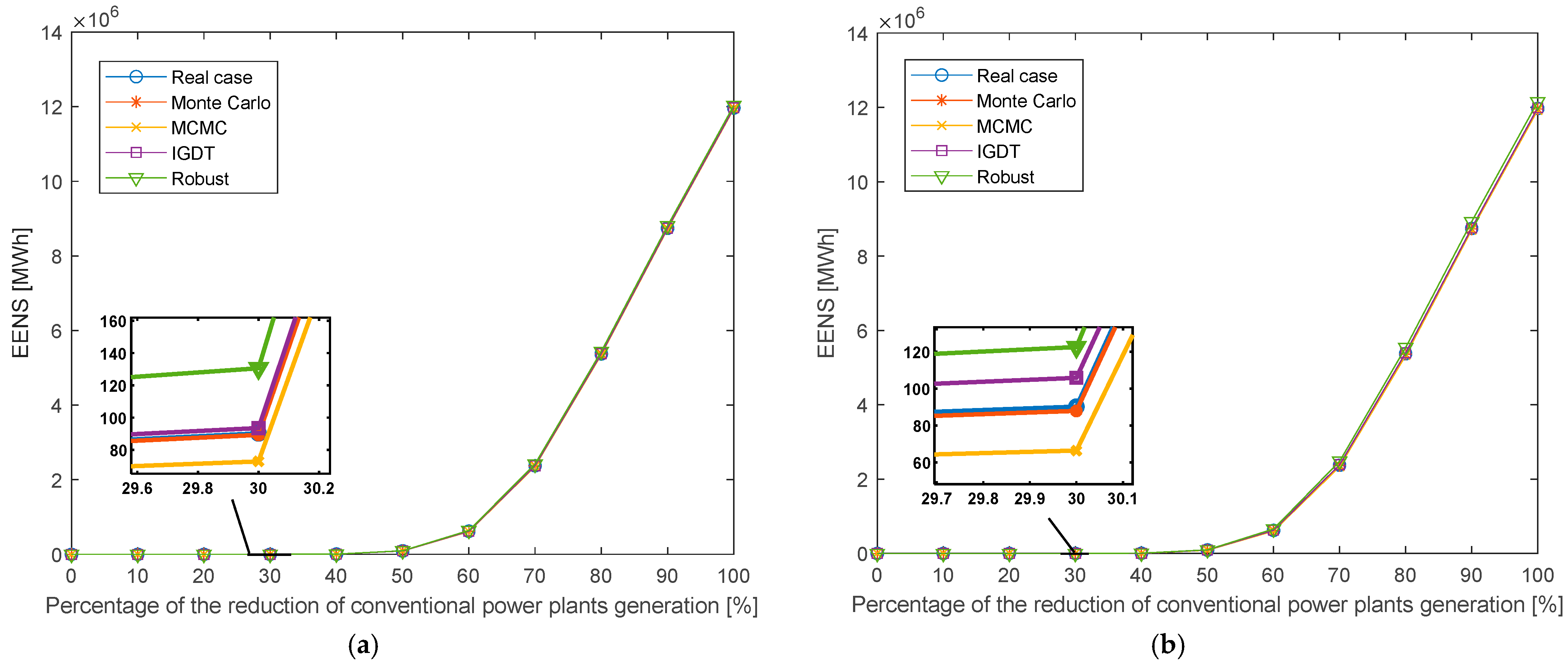
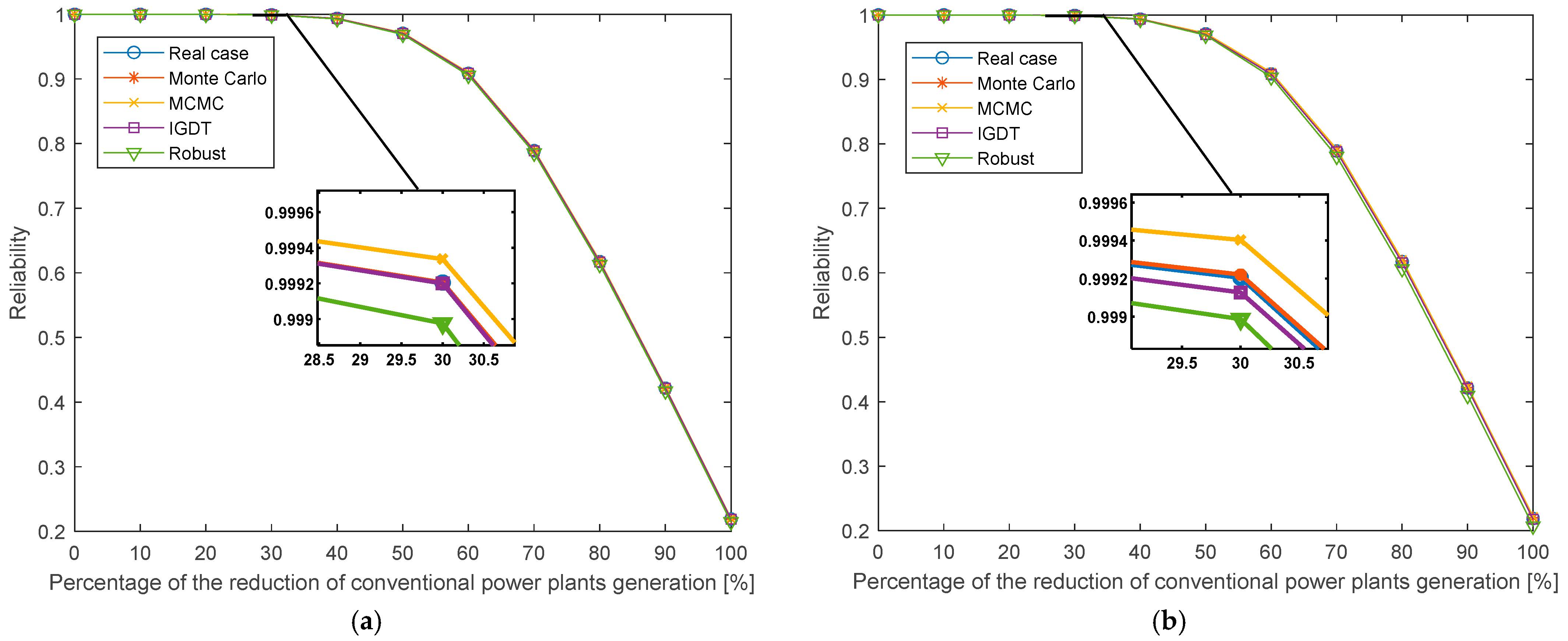
• While most review articles provide theoretical insights, this case study enhances understanding by showing how these methods perform in real-world scenarios. By applying the techniques to a power system integrating wind farms, we assess their impact on key reliability indices such as loss of load expectation (LOLE), loss of load probability (LOLP), and expected energy not supplied (EENS).
• The case study enables a direct, systematic comparison of modeling techniques, such as Monte Carlo simulation, Markov Chain Monte Carlo (MCMC), RO, and IGDT. This practical analysis helps highlight the suitability of different approaches for varying uncertainty durations and levels.
• Presenting practical examples alongside theoretical discussions fosters greater reader engagement, offering a clearer perspective on the applicability of these techniques in real-world challenges.

The main contribution of this paper is evaluating the impact of multiple uncertainty modeling techniques on system reliability and comparing them with a real case in different scenarios of wind farm integration. The case study incorporates different techniques, including Monte Carlo simulation, MCMC, RO, and IGDT, to model the uncertainty of wind speeds and investigate their impact on system performance. This paper contributes not only by comparing these models but also by quantifying their effects on key reliability indices such as LOLE, LOLP, and EENS.

This paper is structured to review risk modeling techniques in Section 2. Uncertainty modeling techniques are discussed in Section 3, the case study is presented in Section 4, and the conclusion is presented in Section 5.

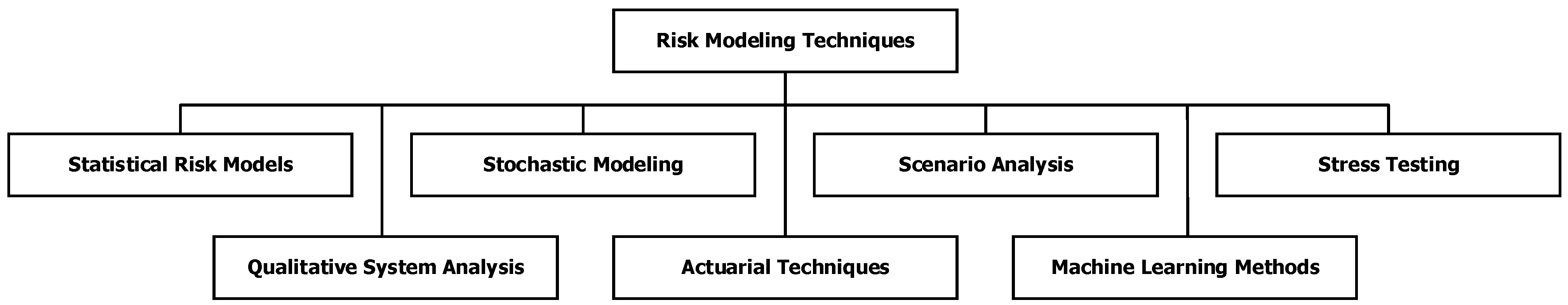
2. Risk Modeling Techniques

Risk modeling techniques are essential tools in power systems, particularly as the integration of RESs introduces significant uncertainties in generation and demand. These techniques allow power system operators, utilities, and decision-makers to identify, quantify, and mitigate risks, ensuring the stability and reliability of the grid. Effective risk modeling is vital in addressing the challenges of fluctuating power generation, load uncertainties, and the growing complexity of power systems. Figure 1 shows an overview of prominent risk modeling techniques applied in power systems.

In the following, each of these risk modeling techniques is discussed.

2.1. Statistical Risk Models

Statistical models use historical data to forecast the probability of future events. These models are commonly employed to estimate the likelihood of various operational risks and uncertainties, which are critical for ensuring the reliability and stability of the grid. In the context of power systems, statistical models are often applied to forecast electricity demand, predict renewable energy output, and assess the risks associated with equipment failures or transmission line outages.

For a portfolio of energy assets or generation units with value $V_i$, a d-dimensional random vector $R_i=\left(R_{i,1},\dots ,R_{i,d}\right)$ of risk factors is often used. The portfolio’s value is given by [5].

$$V_i=f\left(t_i,R_i\right)$$

(1)

where $f$ is a known function and $t_i$ represents the actual time. Typically, risk-factor changes are modeled as $Y_{i+1}=R_{i+1}-R_i$. The resulting loss can be calculated as

$$L_{i+1}=-\left(V_{i+1}-V_i\right)=-\left(f\left(t_{i+1},R_i+Y_{i+1}\right)\right)-f\left(t_i,R_i\right)$$

(2)

This loss can be viewed as the result of applying the operator $l_{\left[i\right]}\left(·\right)$ to the risk-factor changes $Y_{i+1}$:

$$L_{i+1}=l_{\left[i\right]}\left(Y_{i+1}\right)$$

(3)

where

$$l_{\left[i\right]}\left(y\right)=-\left(f\left(t_{i+1},R_i+\mathrm{y}\right)-f\left(t_i,R_i\right)\right)$$

(4)

The operator $l_{\left[i\right]}\left(·\right)$ is known as the loss operator, and $y$ is the risk-factor changes. To linearize the relationship between $L_{i+1}$ and $Y_{i+1}$, we differentiate $f$, resulting in the linearized loss:

$$L_{i+1}^{\mathsf{\Delta }}=-\left(f_t\left(t_i,R_i\right)\mathsf{\Delta }\mathrm{t}+{\sum }_{n=1}^d{f}_{z_n}\left(t_i,R_i\right)Y_{i+1,i}\right)$$

(5)

Here, $f_t\left(t,r\right)={\displaystyle \frac{\partial f\left(t,r\right)}{\partial t}}$ and $f_{z_n}\left(t,r\right)={\displaystyle \frac{\partial f\left(t,r\right)}{\partial z_n}}$. The corresponding operator is given by

$$l_{\left[i\right]}^{\mathsf{\Delta }}\left(y\right)=-\left(f_t\left(t_i,R_i\right)\mathsf{\Delta }\mathrm{t}+{\sum }_{n=1}^d{f}_{z_n}\left(t_i,R_i\right)y_i\right)$$

(6)

in which $l_{\left[i\right]}^{\mathsf{\Delta }}\left(y\right)$ refers to the linearized loss operator.

2.1.1. Statistical Risk Models for Renewable Energies

Risk assessment in renewable power plants involves addressing various technical, environmental, and financial uncertainties. Renewable generation variability can affect energy production predictability, creating uncertainties in power supply. Therefore, a new concept of energy-based availability has been introduced.

Renewable generation availability modeling can be based on either operation time or energy production.

Time-based availability is the percentage of time a system is available compared to the total possible time that it could be available. On the other hand, production-based availability builds on this by also considering the loss of production during downtimes. It measures the actual production in a given time period compared to the maximum possible production if the system operated at full capacity the entire time. Time-based availability is simpler to compute but may not fully capture the risk of energy losses. Production-based availability offers a more accurate representation of these risks if energy values are precise. The time-based availability can be calculated as follows [6]:

$$A_T={\displaystyle \frac{Availabletime\left[\mathrm{hour}\right]}{Totalstudiedtime\left[\mathrm{hour}\right]}}=1-{\displaystyle \frac{Unavailabletime\left[\mathrm{hour}\right]}{\left(\begin{array}{c}Availabletime\\ +Unavailabletime\end{array}\right)\left[\mathrm{hour}\right]}}$$

(7)

where $A_T$ is the time-based availability.

The production-based availability method evaluates energy production as a fraction of expected energy, offering a clearer view of operational risks. It can be modeled as follows [7]:

$$A_P={\displaystyle \frac{Actualenergyproduction\left[\mathrm{kWh}\right]}{Expectedenergyproduction\left[\mathrm{kWh}\right]}}=1-{\displaystyle \frac{Lostproduction\left[\mathrm{kWh}\right]}{\left(\begin{array}{c}Actualenergyproduction\\ +Lostproduction\end{array}\right)[\mathrm{kWh}]}}$$

(8)

where $A_P$ is the production-based availability.

Risk management in renewable energies’ operations involves advanced predictive maintenance, robust design, and operational strategies adapted to specific local conditions. Using sensors and real-time data analytics helps preemptively identify and address potential failures, while designing turbines to withstand local environments and employing flexible operational tactics can mitigate various risks associated with renewable energy production.

Full-time availability of renewable power plants is the ratio of hours deemed available as a fraction of the full period, such as the month or the year. The advantage of full-time availability is considering the effect of maintenance on the availability of renewable power plants.

The full-time availability can be calculated as follows:

$$A_F={\displaystyle \frac{Numberofavailablehours\left[\mathrm{hour}\right]}{Totalperiod\left[\mathrm{hour}\right]}}$$

(9)

where the total period is 8760 h in a year.

2.1.2. Statistical Reliability Models for Power System

The LOLP is the probability that the system’s demand will exceed the available generation capacity at a given time, which results in a loss of load event [8]. The LOLP of a system can be generally expressed as follows [9]:

$$LOLP={\displaystyle \frac{Numberofhourswhere{D}_t>G_t}{T}}$$

(10)

where $D_t$ and $G_t$ are the demand and generation at time $t$, respectively. $T$ is the total studied time period.

Also, the LOLP of a system including spinning reserve (SR) at any time can be calculated as follows:

$${LOLP}_t=\sum _{i\in \Omega }{p}_{i,t}·b_{i,t}$$

(11)

where, $i$ is the index of state, $t$ is the index of time, Ω is the set of scenarios, $p_{i,t}$ is the outage probability, and $b_{i,t}$ can be expressed as follows:

$$b_{i,t}=\left\{\begin{array}{ll}1& if{∆OC}_{i,t}-{SSR}_t>0\\ 0& if{∆OC}_{i,t}-{SSR}_t\le 0\end{array}\right.$$

(12)

where ${∆OC}_{i,t}$ is the outage committed capacity for state $i$ at time $t$ and ${SSR}_t$ is the total system SR at time $t$.

The LOLE is the expected number of hours (or days) within a time period during which the system will experience a loss of load event. It is calculated by summing the probabilities over time intervals. The LOLE can be calculated as follows [10,11,12]:

$$OLE=\sum _{t=1}^T{p}_t\left(C_t-L_t\right)=\sum _{t=1}^T{LOLP}_t,\forall :C_t-L_t<0$$

(13)

where $T$ is generally 8760 h or 365 days, $C_t$ is the available capacity at hour $t$, $L_t$ is the forecasted peak load at hour $t$, and $p_t\left(C_t-L_t\right)$ is the outage capacity cumulative probability, which is equivalent to the probability of loss of load at hour $t$.

The EENS represents the expected amount of energy that cannot be supplied due to insufficient generation capacity over a specific time period [13].

$$EENS=\sum _{t=1}^T{LOLP}_t·\left[D_t-G_t\right]·∆t=\sum _{i\in \Omega }{p}_{i,t}·b_{i,t}·\left[{∆OC}_{i,t}-{SSR}_t\right]$$

(14)

where $D_t-G_t$ is the energy shortfall when demand exceeds generation capacity at time $t$ and $∆t$ represents the time step.

The index of reliability of a system can be expressed as follows [14]:

$$Reliability=1-{\displaystyle \frac{ENS}{D_{total}}}$$

(15)

where ENS and $D_{total}$ are the energy not supplied and the total demand of the system in a specific time period (typically one year), respectively.

The ENS refers to the actual amount of energy demand that is unmet in a specific scenario or time step due to system constraints. On the other hand, the EENS is the statistical expectation of ENS over multiple scenarios, representing a reliability metric that averages the impacts of uncertainties.

2.2. Qualitative System Analysis

Qualitative system analysis is an approach for examining and comprehending complex systems, focusing on their structure, behavior, and interactions without the use of numerical data or mathematical models.

Fault Tree Analysis (FTA) and Markov chains are widely used qualitative system analysis methods in risk modeling, particularly for assessing the reliability and safety of power systems.

FTA is a top-down approach for predicting the probability or frequency of system failures by mapping out various failure modes in a tree-like structure [15]. It helps uncover vulnerabilities by highlighting logical relationships between component failures and system-level risks. The FTA is a deductive method used to analyze potential causes of system failures by systematically breaking down the system into its components [16].

The method of obtaining cut sets is a standard top-down approach for obtaining minimal cut sets in FTA. The process involves the following:

• Start with the top event and break it down using AND/OR gates until basic events are reached.
• Construct a table where each row represents a cut set, and columns represent basic events. Begin by placing the top event in the first row.
• Recursively expand each event in the table:
  • AND gate: Add inputs to new columns within the same row.
  • OR gate: Add inputs to new rows.
• Apply Boolean algebra to eliminate redundant rows and events, isolating minimal cut sets.
• Review and analyze the minimal cut sets to identify critical failure combinations.

This method systematically identifies the smallest combinations of basic events that could lead to the top event, facilitating reliability improvements in complex systems.

On the other hand, the Markov chain approach as a reliability quantification technique can be applied for analyzing how the state of a system may change over time. While time is continuous, the process must satisfy the Markov property. The set of all possible states is referred to as the state space, denoted by $X$. Let the possible states in $X$ be numbered as $\mathrm{0,1},2,\dots ,r$, where the system has $r+1$ different states. Where applicable, assume that state 0 represents the “best” state and state $r$ represents the “worst” state of the system. Let $X\left(t\right)$ represent the state of the system at time $t$. The state $X\left(t\right)$ is a random variable, and $P\left(X\left(t\right)=i\right)=P_i\left(t\right)$ is the probability of the system being in state $i$ at time $t$, for $i=\mathrm{0,1},2,\dots ,r$. The state $X\left(t\right)$ changes over time, making this a stochastic process, specifically referred to as a continuous time Markov process. The combination of Markov chain and Monte Carlo simulation makes a strong method, referred to as MCMC, for modeling the uncertainties in power systems.

2.3. Stochastic Modeling

Stochastic models incorporate randomness directly into their calculations to account for the variability inherent in risk factors. These models are especially prevalent in electricity markets for option pricing or risk assessment in investment portfolios. In the power system sector, stochastic models can be used for modeling the uncertainties in the generation of renewable energies. Stochastic models are vital for understanding the implications of random fluctuations in market prices or interest rates.

Value-at-risk (VaR) is one of the stochastic risk modeling techniques and a widely used risk management tool in finance and power systems. It provides an estimate of the maximum potential loss in value of a risky asset or portfolio over a defined period for a given confidence interval. This technique is commonly employed by banks, investment firms, and corporate risk managers to gauge the amount of assets needed to cover potential losses.

Conditional value-at-risk (CVaR) is raised based on the concept of VaR subject to additional constraints that limit the risk consequences [17]. The CVaR based on a linear function can be expressed by (16) [18].

$$CVaR=VaR-{\displaystyle \frac{1}{1-\alpha }}\sum _{i_1,i_2,\dots ,i_n}\left[{\xi }_{i_1}^{uncertai{n}_{par}}·{\xi }_{i_2}^{uncertai{n}_{par}}·\dots ·{\xi }_{i_n}^{uncertai{n}_{par}}·{\eta }_{i_1,i_2,\dots ,i_n}\right]$$

(16)

where ${\xi }_{i_n}^{uncertai{n}_{par}}$ is the probability of the n-th uncertain parameter.

The constraints for CVaR are presented in (17) and (18).

$$VaR-f_{i_1,i_2,\dots ,i_n}\le {\eta }_{i_1,i_2,\dots ,i_n}$$

(17)

$${\eta }_{i_1,i_2,\dots ,i_n}\ge 0$$

(18)

Figure 2 demonstrates the calculation of CVaR, showing the probability distribution of losses in an investment portfolio. The area shaded in red represents the tail of the distribution beyond the VaR threshold, where CVaR is calculated. This shaded area corresponds to the expected average loss in the worst-case scenarios beyond the VaR point, effectively highlighting the extreme losses that could occur, which CVaR aims to quantify and manage.

2.4. Actuarial Techniques

Actuarial techniques are being applied in power systems to manage risks associated with uncertainty in generation, demand, and equipment reliability. These methods use mathematical and statistical tools to model risks and forecast potential system failures or financial losses due to outages. For instance, techniques like life-table methods can assess system component failure rates, while loss modeling helps evaluate risks in cases of extreme weather affecting grid stability. The equivalence principle, commonly used in actuarial science, can be adapted to determine expected operational costs and allocate resources efficiently in power systems. By leveraging the law of large numbers, these techniques provide stronger predictions of system behavior under uncertain conditions, enhancing decision-making in grid management. Applications of these techniques help utilities optimize reliability, resource allocation, and risk mitigation strategies, particularly as renewable energy integration introduces more variability into power systems. The law of large numbers (LLN), as one of the most famous actuarial techniques, posits that as the number of exposures increases, the actual results will progressively align with the expected results [19]. The simplest principle of the actuarial valuation is the so-called equivalence principle, which can be described as follows [20]:

$$\pi \left(X\right)=\mathbb{E}\left(X\right)$$

(19)

where $\pi$ is the equivalence premiums and $X$ has a distribution with a finite mean. The LLN states that

$${\displaystyle \frac{1}{n}}\sum _{i=1}^n{X}_i\to \mathbb{E}(X)\left(n\to \mathrm{\infty }\right)$$

(20)

In this case, the probability convergence is as follows:

$$\underset{n\to \mathrm{\infty }}{\lim }\mathbb{p}\left(\left|\mathbb{E}\left(X\right)-{\displaystyle \frac{1}{n}}\sum _{i=1}^n{X}_i\right|\ge ϵ\right)=0,\forall ϵ>0$$

(21)

On the other hand, the assured convergence can be presented as follows:

$$\mathbb{p}\left(\underset{n\to \mathrm{\infty }}{\mathrm{l}\mathrm{i}\mathrm{m}}{\displaystyle \frac{1}{n}}\sum _{i=1}^n{X}_i=\mathbb{E}(X)\right)=1$$

(22)

The assured convergence implies convergence in probability, making it a stronger result. This stronger result is known as the strong LLN.

2.5. Scenario Analysis

Scenario analysis in power systems involves forecasting the outcomes of different potential future scenarios to evaluate risks and impacts on system operations. This method is particularly valuable in planning and managing power grids, as it allows system operators to simulate various conditions, such as changes in energy demand, renewable generation variability, and equipment failures. By considering worst-case and best-case scenarios, power utilities can better prepare for operational challenges, enhance grid resilience, and optimize strategies to ensure reliable and efficient energy delivery under uncertain conditions.

Monte Carlo simulation is one of the prominent methods for scenario reduction and analysis, and its formulation is discussed in Section 3.1.1.

2.6. Machine Learning Techniques

Recent advancements in machine learning have led to its application in risk modeling. These techniques can identify patterns and predict outcomes from large datasets, such as wind speed and solar irradiance data, where traditional statistical methods might not be effective. Deep learning is one of the machine learning methods that are based on neural networks and often has a complex hidden layer structure with a variety of different layers. Typically, the first layer uses a linear transfer function to obtain activation parameters, which is shown in (23) [21].

$$a_i=b_i+\sum _{j=1}^n{x}_j{\mathrm{ⱳ}}_{i,j}\forall i=1,\dots ,m$$

(23)

where $a_i$, $b_i$, $x_j$, and ${ⱳ}_{i,j}$ are the activation, bias, input, and model weight, respectively.

The activation parameters transform by an activation transfer function ($g$) within the hidden layers as follows:

$$y_i=g\left(a_i\right)$$

(24)

where $y_i$ is the hidden unit. The hidden units should be combined to obtain the activation of the output layer, which is shown as follows:

$$a_o=b_{\mathrm{o}}+\sum _{j=1}^n{y}_j{\mathrm{ⱳ}}_{\mathrm{o},j}$$

(25)

where $a_o$, $b_o$, and ${ⱳ}_{o,j}$ are the activation, bias, and model weight of the output layer, respectively. Finally, the activation function g and a risk factor ($R$) can be applied to obtain the final output $Y$ as follows:

$$Y=f\left(a_o\right)·R$$

(26)

By having $x_j$ and obtaining $Y$, the deep neural network can be trained to minimize the final loss function in a supervised way. This training enables the network to predict $Y$ based on new inputs $x_j$.

2.7. Stress Testing

Stress testing involves simulating extreme conditions to evaluate how different assets or systems perform under stress. Stress testing is applicable to some areas in the electrical engineering sector, such as the printed circuit board assembly (PCBA) process. Moreover stress testing assesses the risks associated with critical infrastructure (CI). The CI performance changes over time due to aging, hazards, or events, impacting functionality. The grading system accounts for this, making stress tests periodic. Passing with grade AA or A keeps risk objectives until the next test, with intervals set by the regulator. Most CIs get grade B or C, indicating high risk. To promote upgrades, stricter objectives or shorter test intervals are used, aiming for grade A or CI termination. Redefining risk objectives requires identifying the characteristic point of risk, which guides future grading. This point is the highest risk above the ALARP region on the F-N curve. If grade B is obtained in the first test (ST1), the B-C boundary will be adjusted in the next test (ST2) to reflect risk levels beyond the ALARP region, ensuring risk equity across cycles. This ensures risk equity over two cycles and can be expressed as follows [22]:

$$R_{ST1}-R_{\left(A-B\right)}=R_{\left(B-C\right),ST1}-R_{\left(B-C\right),ST2}$$

(27)

$R_{\left(A-B\right)}$ is the A-B boundary, $R_{\left(B-C\right),ST1}$ and $R_{\left(B-C\right),ST2}$ are the B-C boundaries in ST1 and ST2, and RST1 is the risk measure in ST1. The left side of Equation (27) represents the risk beyond the ALARP region in ST1. If grade C is given in ST1, the B-C boundary and the period until ST2 are reduced. The B-C boundary is set to the A-B boundary, which is the maximum reduction. The reduced period until ST2 ($t_{cycle,redefined}$) ensures risk equity over two cycles and is calculated as follows:

$$t_{cycle,redefined}=\left[t_{cycle,initial}·{\displaystyle \frac{R_{\left(B-C\right),ST1}-R_{\left(A-B\right)}}{R_{ST1}-R_{\left(A-B\right)}}}\right]$$

(28)

where $t_{cycle,initial}$ is the initial duration between two stress tests.

Risk modeling techniques are essential for organizations to effectively identify, assess, and manage potential risks. By utilizing these methods, companies can make informed decisions, minimize losses, and adapt to unexpected challenges, ensuring their operations remain resilient, sustainable, and reliable.

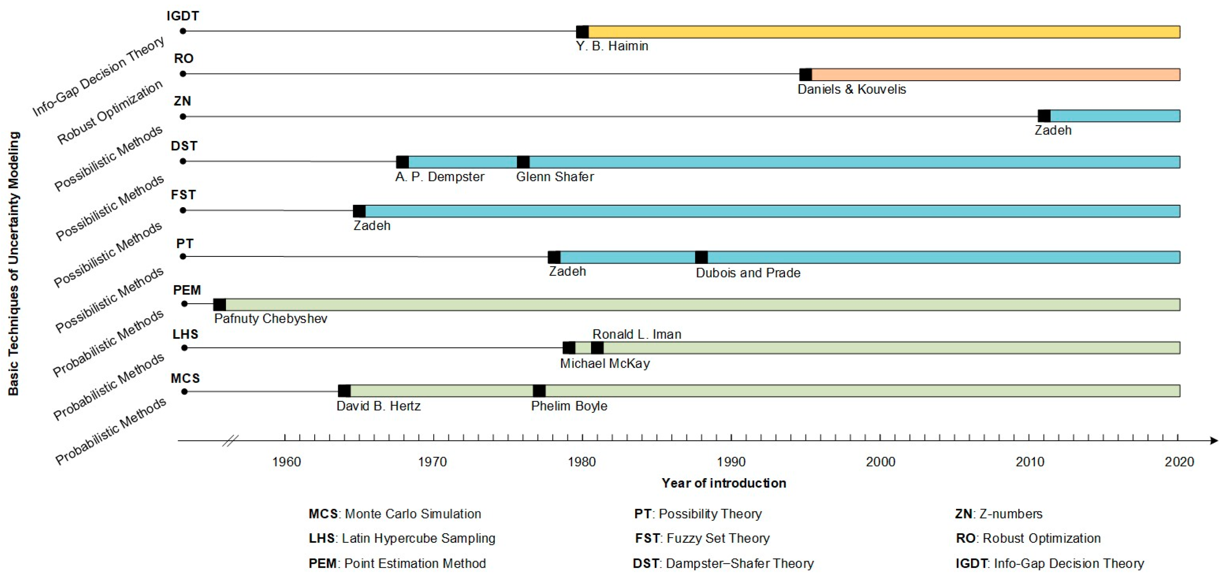
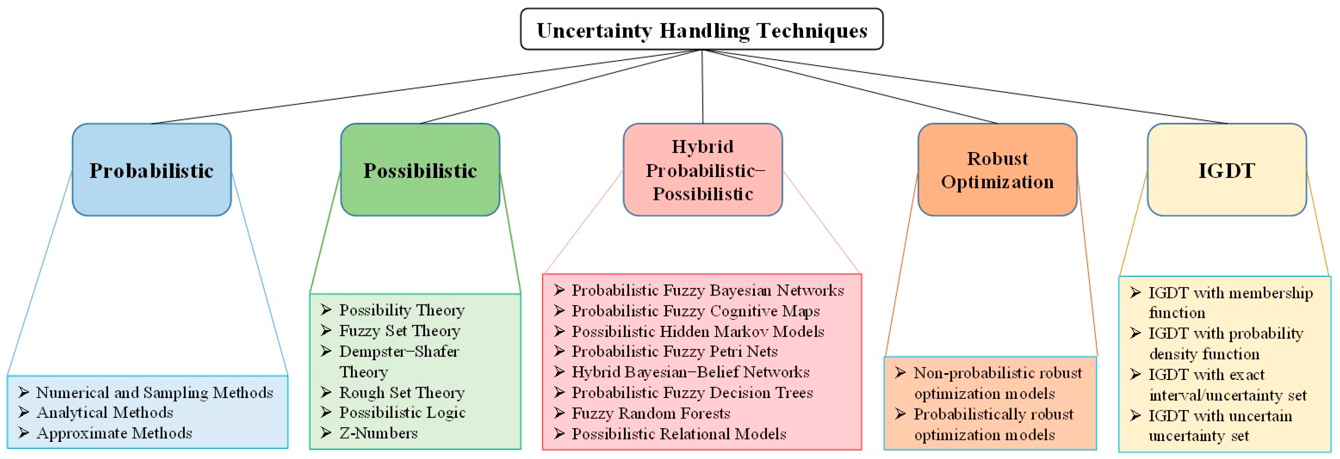
3. Uncertainty Modeling Techniques

Uncertainty modeling techniques address the degree of uncertainty involved in the predictions and outcomes of various models, which is primarily due to incomplete or imperfect information about the systems being modeled. Figure 3 presents a timeline that illustrates the development and introduction of various methods used in uncertainty quantification. Spanning from the early 19th century to the modern era, it highlights key methodologies such as Monte Carlo simulation, probability theory, fuzzy set theory, and IGDT, among others. Notable contributors and their key works are annotated alongside the respective methodologies they influenced or introduced.

Figure 4 shows the various uncertainty modeling techniques, including probabilistic, possibilistic, hybrid probabilistic–possibilistic, robust optimization, and IGDT. In the following, each category is discussed.

3.1. Probabilistic Methods

Probabilistic methods are fundamental to uncertainty modeling in power systems, using probability theory to evaluate the likelihood of various outcomes under uncertain conditions. These methods can be divided into analytical, numerical, and sampling approaches. Analytical methods compute probabilities directly using predefined distributions, suitable for systems with well-defined parameters. In complex power systems where analytical solutions are difficult, numerical methods, such as Monte Carlo simulations, are employed. These simulations use random sampling to estimate outcome probabilities, addressing both aleatory and epistemic uncertainties by evaluating a wide range of scenarios.

3.1.1. Numerical and Sampling Methods

Numerical and sampling methods are extensively applied in uncertainty modeling to manage and analyze the variability in systems and predictions. Numerical methods involve algorithms for solving mathematical problems through approximate solutions and are especially useful when exact solutions are unattainable. Monte Carlo simulation is particularly effective for modeling uncertainty, relying on repeated random sampling to assess risks in complex scenarios with multiple uncertain variables. Another advanced sampling technique, Latin Hypercube Sampling (LHS), improves upon Monte Carlo simulation by dividing the input distribution into equally probable intervals, ensuring comprehensive sampling across all segments. This method increases efficiency and accuracy, especially in multidimensional power system models, making both Monte Carlo and LHS valuable tools for uncertainty quantification and risk management in power grid operations.

A. 

Monte Carlo Simulation

The integration of Monte Carlo simulation with photovoltaic systems has garnered attention due to the need for robust tracking techniques under variable environmental conditions, such as partial shading.

In [23], a heuristic approach combined with Monte Carlo simulations for optimizing the reliability and cost of stand-alone photovoltaic systems in off-grid areas is introduced. The method efficiently sizes PV installations, achieving high reliability and minimized costs with low iteration requirements. In [24], Hamiltonian Monte Carlo is introduced to enhance sampling efficiency and accuracy for voltage sag assessments, outperforming traditional methods like importance sampling and Metropolis–Hastings. Reference [25] has used the Monte Carlo simulation for the techno-economic evaluation of energy storage systems in concentrated solar power plants, demonstrating that combined sensible–latent heat storage systems have the lowest levelized cost of electricity and uncertainty.

To estimate the expected value of a random variable ($X$) by Monte Carlo simulation, the probability distributions for all input variables should be determined. Let us assume that there are n random variables $X_1,X_2,\dots ,X_n$, each with known probability distributions $P_{X_1},P_{X_2},\dots ,P_{X_n}$. A number of simulations ($M$), which often is a large number, should be conducted to compute the output variable. For each simulation i, a set of random values ($x_1^{\left(i\right)},x_2^{\left(i\right)},\dots ,x_n^{\left(i\right)}$) based on their probability distribution should be generated. The output variable ($Y$) as a function of the input variables can be described as follows [26]:

$$y^{\left(i\right)}=f(x_1^{\left(i\right)},x_2^{\left(i\right)},\dots ,x_n^{\left(i\right)})$$

(29)

To analyze the results, the expected value of outputs can be calculated as follows:

$$\mathbb{E}\left(Y\right)={\displaystyle \frac{1}{M}}\sum _{i=1}^M{y}^{\left(i\right)}$$

(30)

B. 

Latin Hypercube Sampling (LHS)

LHS is a statistical method that improves upon random sampling by ensuring that the entire range of possible values is evenly sampled across all dimensions. This method is highly efficient for estimating uncertainties in simulations with fewer samples and is commonly used in engineering and risk analysis. The uncertainty quantification of nuclear steam supply systems, particularly small pressurized water reactors (SPWRs) with once-through steam generators (OTSGs), has gained significant attention. A nonlinear mathematical model incorporating the reactor core, OTSG, and pressurizer models is established in [27]. A control strategy maintaining a constant reactor core coolant temperature and secondary-side outlet pressure of the OTSG was adopted. Leveraging LHS and statistical methods, they developed a quantitative platform for parameter uncertainty, showcasing its application on the primary-side flow rate of the OTSG under variable loads and step disturbances. Results indicated acceptable maximum uncertainties for SPWR critical output parameters. In [28], an overview of uncertainty and sensitivity analysis techniques is provided, emphasizing LHS within Monte Carlo analysis. The LHS has been applied in power systems to enhance reliability assessments and optimize system designs. In [29], LHS is integrated into an extendable Latin hypercube importance sampling (ELHIS) method to address the computational challenges of evaluating the reliability of power systems with renewable energy integration. By combining LHS with importance sampling, and leveraging cross entropy theory and Gaussian mixture models, the method improves the accuracy of sampling and reduces computational costs. The ELHIS approach is tested on a power system with real data from wind farms and photovoltaic stations, demonstrating faster and more efficient reliability assessments compared to traditional importance sampling methods. In [30], LHS is used alongside Grey Relational Analysis (GRA) for the optimization of a battery thermal management system. This study applies LHS to explore the design parameters of a liquid cooling system, such as mass flow rate and channel dimensions, to minimize pressure drop and temperature, while maximizing convective heat transfer. The optimized design, achieved through LHS and GRA, shows a significant improvement in cooling performance.

LHS is a method that draws on the principles of stratified sampling. In LHS, stratification is applied solely to the marginal distributions. This involves dividing each random variable $X$ into $N$ consecutive intervals, each with an equal probability as defined by the cumulative distribution function $F\left(X\right)$. To facilitate this, the unit interval [0,1] is split into $N$ equal segments, each with a probability of $1/N$. The boundaries of these segments are marked by lower (${\varphi }_{k-1}$) and upper (${\varphi }_k$) bounds, where the upper bound can be calculated as follows [31]:

$${\varphi }_k={\displaystyle \frac{k}{N}},k=1,\dots ,N$$

(31)

The bounds for each interval across the values of $X$ can be determined by the inverse of $F\left(X\right)$ as follows:

$${\xi }_k=F^{-1}\left({\varphi }_k\right)$$

(32)

One scenario, $x_k$, must be chosen within each interval, ensuring that $x_k\in \left({\xi }_{k-1}{,\xi }_k\right)$.

There are different variations of LHS, including random, mean, and median LHS, which differ in how the samples are selected within each probability interval. In median LHS, the sampling probabilities for each interval are defined as follows:

$$P=\left(p_1,p_2,,\dots ,p_k,\dots ,p_N\right),p_k={\displaystyle \frac{k-0.5}{N}}$$

(33)

The samples are then selected using the inverse function of these probabilities as follows:

$$x_k=F^{-1}\left(p_k\right)$$

(34)

For mean LHS, the method focuses on selecting the mean within each interval, which necessitates a numerical integration of the probability density function $f\left(X\right)$ to compute these means. This methodological approach ensures a thorough coverage and representation of the distribution’s range, enhancing the sampling’s efficiency and accuracy.

3.1.2. Analytical Methods

Analytical methods for uncertainty modeling in power systems offer mathematical frameworks to predict and manage the variability in power generation and demand, and PEMs are one of these key methodologies. PEMs are widely used to estimate an unknown parameter of a population using sample data. The goal of point estimation is to provide a single best guess or value for a parameter, such as the population mean or variance, based on observed data.

A. 

Point Estimation Methods (PEMs)

PEMs have been increasingly applied in power systems to address uncertainty, particularly with the rise in renewable energy sources such as wind and distributed generation (DG). The improved multi-PEM proposed in [32] is specifically tailored for probabilistic transient stability assessments in systems with wind power. By leveraging an extreme learning machine to model wind power uncertainty and utilizing a Gauss–Hermite integral-based approach, this method improves the accuracy of stability predictions without sacrificing computational efficiency. Similarly, in the context of power system state estimation, the proposed method in [33] combines kernel-based objective functions with a primal–dual Interior Point approach to optimize the similarity between actual and estimated states. This method offers significant advantages, such as addressing leverage points and identifying bad data, which are critical for accurate state estimation. Lastly, the application of an improved three-PEM and maximum entropy theory in [34] addresses the probabilistic harmonic power flow in distribution networks with DG. This approach transforms probabilistic problems into deterministic ones, improving the accuracy of harmonic voltage distribution calculations.

The method of point estimation focuses on distilling the statistical data from the initial central moments of a random variable into $i$ points for each variable, a process known as concentration. A specific application of this method is the two-point estimate method (2PEM). This approach involves a mathematical formulation, in which initial values are assigned in the first step as follows [35]:

$${\mathbb{E}\left(Y\right)}^{\left(1\right)}=0;{\mathbb{E}\left(Y^2\right)}^{\left(1\right)}=0$$

(35)

In the second step, the positions and probabilities of two concentrations are determined using (36a) and (36b).

$$\begin{gathered} {\xi }_{k,1}={\displaystyle \frac{{\lambda }_{k,3}}{2}}+\sqrt{n+{\left({\displaystyle \frac{{\lambda }_{k,3}}{2}}\right)}^2},k=1,\dots ,n \\ {\xi }_{k,2}={\displaystyle \frac{{\lambda }_{k,3}}{2}}-\sqrt{n+{\left({\displaystyle \frac{{\lambda }_{k,3}}{2}}\right)}^2},k=1,\dots ,n \end{gathered}$$

(36a)

$$\begin{gathered} P_{k,1}={\displaystyle \frac{{\xi }_{k,2}}{2n\sqrt{n+{\left(\frac{{\lambda }_{k,3}}{2}\right)}^2}}},k=1,\dots ,n \\ {P}_{k,2}={\displaystyle \frac{-{\xi }_{k,1}}{2n\sqrt{n+{\left(\frac{{\lambda }_{k,3}}{2}\right)}^2}}},k=1,\dots ,n \end{gathered}$$

(36b)

where ${\xi }_{k,1}$ and ${\xi }_{k,2}$ are unknown constants that should be determined and ${\lambda }_{k,3}=P_{k,1}·{{\xi }_{k,1}}^3+P_{k,2}·{{\xi }_{k,2}}^3.$ $P_{k,1}$ and $P_{k,2}$ are the probabilities of concentrations at locations $x_{k,1}$ and $x_{k,2}$, respectively.

The concentrations’ locations, $x_{k,1}$ and $x_{k,2}$, can be calculated as follows:

$$\begin{gathered} x_{k,1}={\mu }_{X,k}+{\xi }_{k,1}·{\sigma }_{X,k} \\ {x}_{k,2}={\mu }_{X,k}+{\xi }_{k,2}·{\sigma }_{X,k} \end{gathered}$$

(37)

where ${\mu }_{X,k}$ and ${\sigma }_{X,k}$ represent the mean and variance of the $k$-th random variable, respectively.

The output variable in relation to vector $X$ can be calculated as follows:

$$Y=f\left(X\right)$$

(38a)

$$X=\left[{\mu }_{k,1},\dots ,{\mu }_{k,i},\dots ,{\mu }_{k,n}\right],\forall i\in \left\{\mathrm{1,2}\right\}$$

(38b)

Further, Equations (39a) and (39b) should be calculated:

$${\mathbb{E}\left(Y\right)}^{k+1}\cong {\mathbb{E}\left(Y\right)}^k+\sum _{i=1}^2{P}_{k,i}·h\left(X\right)$$

(39a)

$${\mathbb{E}\left(Y^2\right)}^{k+1}\cong {\mathbb{E}\left(Y^2\right)}^k+\sum _{i=1}^2{P}_{k,i}·h^2\left(X\right)$$

(39b)

Finally, for statistical analysis provided by the two-point estimate method, the expected value and standard deviation of $Y$ can be shown as follows:

$${\psi }_Y=\mathbb{E}\left(\mathrm{Y}\right)$$

(40a)

$${\sigma }_Y=\sqrt{\mathbb{E}\left({\mathrm{Y}}^2\right)-{\left({\psi }_Y\right)}^2}$$

(40b)

3.2. Possibilistic Methods

Possibilistic methods offer a framework for dealing with uncertainty where classical probabilistic methods may be inadequate or inapplicable. Unlike probability theory, which quantifies uncertainty in terms of likelihoods, possibilistic approaches focus on the degrees of possibility, typically representing uncertainty without requiring precise statistical data. These methods are particularly useful in handling incomplete, imprecise, or non-statistical data.

3.2.1. Possibility Theory

Possibility theory is grounded in fuzzy logic, extending it to handle uncertainty and partial truth. It is characterized by possibility and necessity measures that express how feasible a particular event or condition is within a given context. This theory is applied extensively in decision-making processes, especially under conditions of uncertainty and vague information.

Possibility theory has gained traction in power systems, particularly for handling uncertainty and imprecise information. In [36], possibility theory is employed alongside fuzzy numbers to tackle power flow problems that arise due to incomplete, inaccurate, or redundant data. This approach allows for the modeling of nested information—common in electrical networks due to varying levels of measurement accuracy—by formalizing the problem as an AC fuzzy power flow model. The method efficiently solves nonlinear fuzzy systems and demonstrates robustness and accuracy in benchmark simulations, making it well suited for real-world applications with uncertain data. In the domain of risk analysis, possibility theory is integrated with Failure Mode and Effects Analysis (FMEA) in [37] to improve the prioritization of failure modes. Traditional FMEA approaches struggle with overlapping risk membership functions, but by utilizing fuzzy similarity values and possibility theory, the method ensures that failure modes with similar risk levels are grouped more naturally without requiring arbitrary defuzzification. This integration enhances robustness and conformance in risk assessments, as demonstrated through case studies.

The $\alpha$-cut method is one of the possibilistic methods, which can be used to calculate the possibility distribution of the possibilistic output variable ($\tilde{Y}$) of uncertain input variables ($\tilde{X}$). $\tilde{Y}$ can be represented in the form of a multi-variable function as follows:

$$\tilde{Y}=h({\tilde{X}}_1,{\tilde{X}}_2,\dots ,{\tilde{X}}_N)$$

(41)

When the possibility distributions of the uncertain input variables $\tilde{X}$ are known, the possibility distribution of $\tilde{Y}$ can be determined using the α-cut method. For a given input variable, the α-cut of $\tilde{X}$ is determined as follows:

$$A^{\mathsf{\alpha }}=\{x\in Uǀ{\pi }_{\tilde{X}}\left(x\right)\ge \alpha ,0\le \alpha \le 1\}$$

(42)

$$A^{\mathsf{\alpha }}=[{\underset{\_}{A}}^{\mathsf{\alpha }},{\overline{A}}^{\mathsf{\alpha }}]$$

(43)

Here, $U$ represents the universe of discourse for $\tilde{X}$, or the range of its possible values, and ${\underset{\_}{A}}^{\mathsf{\alpha }}$ and ${\overline{A}}^{\mathsf{\alpha }}$ denote the lower and upper bounds of $A^{\mathsf{\alpha }}$, respectively. In Figure 5, a typical α-cut for a trapezoidal membership function is illustrated.

3.2.2. Fuzzy Set Theory

Fuzzy set theory, introduced by Lotfi Zadeh, forms the basis of many possibilistic methods by allowing elements to have varying degrees of membership in a set, rather than being restricted to binary membership as in traditional set theory. This approach is widely used in systems that need to handle ambiguous or continuous data.

Recent advancements in fuzzy set theory and its applications in uncertainty management are highlighted in two pivotal studies. In [38], the research shifts from conventional type-1 fuzzy sets to type-2 fuzzy sets to better accommodate high levels of linguistic and numerical uncertainties, which are prevalent in practical applications such as the reliability evaluation of phasor measurement units. The study emphasizes the effectiveness of type-2 fuzzy sets, which incorporate secondary membership functions to handle these uncertainties, proving to be a superior method especially in contexts with insufficient field data. In [39], climate change mitigation by nuclear energy is discussed. This reference has used the nonlinear fuzzy set theory for the assessment of climate change.

A fuzzy set $\tilde{A}$ in the universe of information U can be defined as a collection of ordered pairs, mathematically expressed as follows:

$$\tilde{A}=\left\{\left(y,{\mu }_{\tilde{A}}\left(y\right)\right)ǀy\in U\right\}$$

(44)

Here, ${\mu }_{\tilde{A}}\left(y\right)$ = degree of membership of $y$ in $\tilde{A}$, assuming values in the range from 0 to 1, i.e., ${\mu }_{\tilde{A}}\left(y\right)\in \left[\mathrm{0,1}\right]$.

3.2.3. Dempster–Shafer Theory (DST)

DST offers a framework for combining evidence from different sources to arrive at a degree of belief (represented by a belief function) that takes into account all the available evidence. Unlike traditional probability, it does not require mutually exclusive and exhaustive hypotheses and can operate under less information.

DST has been effectively applied in power systems, particularly for decision-making and uncertainty analysis. In [40], DST is utilized to address the complex multi-criteria decision-making (MCDM) process involved in selecting optimal offshore wind turbines. This method accommodates the uncertainty inherent in expert judgments, representing them as basic probability assignments and fusing them using DST synthesis rules. By applying DST in conjunction with the stepwise weighted assessment ratio analysis, the study demonstrates how the best turbine can be selected from multiple alternatives under uncertain conditions. This DST-based MCDM framework is particularly useful for projects with high complexity and uncertain data inputs, such as offshore wind farms. In [41], DST is extended to uncertainty and sensitivity analysis for building energy assessments. Since traditional probabilistic methods cannot handle situations where there is insufficient information to define precise probabilities, DST offers an alternative by constructing belief and plausibility measures based on interval-valued probabilities. This allows for more nuanced uncertainty modeling in scenarios where data are incomplete or imprecise. The combination of DST with machine learning techniques in building energy simulations further enhances the robustness and reliability of uncertainty assessments.

The basic probability assignment, denoted by m, is a function from the power set of the universal set X to the interval [0,1]. It adheres to the following conditions [42]:

$$m:P\left(X\right)\to \left[\mathrm{0,1}\right]$$

(45)

$$m\left(\theta \right)=0$$

(46)

$$\sum _{A\in P\left(X\right)}m\left(A\right)=1$$

(47)

where $P\left(X\right)$ represents the power set of $X$, $\theta$ is the null set, and $A$ is a set in the power set ($A\in P\left(X\right)$).

In defining the measures for uncertainty, the belief (Bel) of a set A is computed as the cumulative basic probability assignments (BPAs) for all proper subsets contained within $A$, expressed mathematically as

$$Bel\left(A\right)=\sum _{B\left|B\underset{\_}{⸦}A\right.}m\left(B\right)$$

(48)

Conversely, plausibility (Pl) encompasses the sum of BPAs for all sets that have a non-empty intersection with $A$, formulated as

$$Pl\left(A\right)=\sum _{B\left|B\cap A\ne \varnothing \right.}m\left(B\right)$$

(49)

Both belief and plausibility are non-additive measures; thus, their sums do not necessarily equate to 1. This non-additivity implies that complete knowledge of one measure does not infer the total of the other.

Additionally, the relationship between belief and its BPA is inverse, allowing for the derivation of BPA from Bel. Furthermore, plausibility can be derived from belief through the complement rule:

$$Pl\left(A\right)=1-Bel\left(\overline{A}\right)$$

(50)

These measures, by bounding the precise classical probability of an event, provide lower and upper limits, respectively, where the precise probability is uniquely determined if $Bel\left(A\right)=Pl\left(A\right)$. This relationship emphasizes the theoretical underpinnings of uncertainty quantification in evidential reasoning frameworks.

3.2.4. Z-Numbers

Z-numbers are an extension of fuzzy numbers that include a measure of certainty about the provided information. This allows them to be more effective in environments where the reliability of data is questionable, enhancing decision-making processes under uncertainty.

Z-numbers, which integrate both the reliability and uncertainty of information, have been effectively applied in power systems for decision-making in complex and uncertain environments. In [43], a Z-number-based framework is used for the site selection of electric vehicle (EV) battery swapping stations. By combining K-Means clustering with a multi-criteria decision-making method under the Z-number environment, the framework accounts for uncertainty in evaluating alternative sites. In [44], Z-numbers are used in supplier selection to address uncertainty in the context of green, resilient, and inclusive development. The enhanced best-worst method and TOPSIS, integrated with scenario-varying Z-numbers, assess suppliers under dependent uncertain events. By assigning Z-numbers to different criteria, the model improves the reliability of rankings in uncertain scenarios.

A Z-number is defined as an ordered pair $Z=(A,B)$, where $A$ is a fuzzy set that imposes a restriction on the possible values of an uncertain variable $X$, denoted by $X$ as $A$. This restriction is characterized by a fuzzy membership function ${\mu }_A\left(u\right)$, which quantifies the degree of compatibility of each value $u$ with the fuzzy set $A$. $B$ quantifies the reliability or certainty of the restriction provided by $A$, usually expressed in terms of a linguistic variable, such as “very sure” or “likely”.

The possibilistic restriction on the variable $X$, imposed by $A$, can be expressed as [45]

$$R\left(X\right):XisA⟹Poss\left(X=u\right)={\mu }_A\left(u\right)$$

(51)

where ${\mu }_A\left(u\right)$ is the membership function of the fuzzy set $A$, and $u$ represents a generic value of $X$.

When $X$ is considered as a random variable, its probability distribution acts as a probabilistic restriction on $X$. This probabilistic restriction can be mathematically expressed as $R\left(X\right):Xisp$, where $p$ represents the probability density function of $X$. Consequently, for a small interval around $u$, the probability that $X$ takes a value within [$u,u+du$] is given by

$$R\left(X\right):Xisp⟹Prob\left(u\le X\le u+du\right)=p_X\left(u\right)du$$

(52)

The relationship between $X$ and $A$ can be extended to include a restriction on the probability measure of A as $R\left(X\right):XisA$ and $Prob\left(XisA\right)isB$, where $B$ evaluates the confidence level in the fuzzy restriction provided by $A$. Figure 6 shows a simple Z-number with the membership function ${\mu }_A$.

3.3. Hybrid Probabilistic–Possibilistic Methods

Hybrid probabilistic–possibilistic methods have emerged as powerful tools for addressing uncertainties in power systems, particularly in scenarios where both exogenous and endogenous uncertainties play significant roles. In [46], a hybrid framework is introduced to evaluate the capacity credit of demand response (DR) in smart grids by combining probabilistic and possibilistic models to capture uncertainties from both physical and human factors. This approach enables a more comprehensive assessment of DR’s reliability potential, factoring in variables like load participation and recovery. In [47], a hybrid method is employed to manage the risk of high-impact, low-probability (HILP) events in power system self-scheduling. Probabilistic models capture the stochastic nature of wind power, while possibilistic models address forced outages due to extreme events. This allows for a more resilient scheduling strategy that accounts for both common and rare events. In [48], a hybrid probabilistic-possibilistic flexibility-based unit commitment model incorporates Z-numbers to manage the uncertainty of DR resources alongside supply-side uncertainties. This method optimizes system flexibility and reduces operational costs. Furthermore, [49] combines probabilistic approaches with IGDT for energy management in active distribution networks, balancing uncertainties in load, renewable generation, and grid prices while improving operational efficiency. Reference [50] presents a hybrid scenario-based/IGDT method for optimizing multi-carrier energy systems, effectively addressing uncertainties in both renewable energy sources and electricity prices. These applications demonstrate the versatility of hybrid probabilistic–possibilistic methods in power systems, enabling more reliable and resilient operations under varying uncertainty conditions.

3.4. Robust Optimization (RO)

RO has become an indispensable tool in power systems for managing uncertainties and improving system resilience. In [51], a two-stage RO approach is introduced to assess the flexibility capacity of new power systems, focusing on balancing supply and demand while optimizing ramping capabilities and operating costs. Similarly, [52] applies a distributionally robust resilience optimization model to address uncertainties in post-disaster power system restoration, using stochastic programming combined with a Wasserstein distance-based ambiguity set to improve recovery strategies. For wind power integration, [53] proposes a data-driven distributionally RO approach that captures spatial correlations between wind farms, resulting in more accurate and cost-effective dispatching decisions for multi-resource grids. In [54], a multi-resource reserve RO model integrates wind power frequency regulation potential, improving system flexibility and frequency stability through a column-and-constraint generation algorithm. Expanding on inter-regional planning, [55] combines stochastic and RO methods to handle uncertainties in generation and transmission planning for the ASEAN region, leading to a cost reduction of 6.0% by leveraging cross-border renewable energy. Reference [56] introduces an RO model for aggregating active distribution systems into virtual power plants (VPPs), addressing uncertainties in renewable generation and dispatch orders. These studies demonstrate the versatility of RO in addressing uncertainties across different domains in power systems.

Figure 7 compares RO with traditional optimization. Solution A, derived from traditional optimization, excels in optimality but shows considerable variation in the objective function relative to changes in the design variable, potentially extending into infeasible ranges. On the other hand, Solution B, achieved through RO, demonstrates moderate optimality and excels in robustness, maintaining a narrow dispersion in the objective function as the design variable varies.

A typical optimization problem with uncertainty can be written as [57]

$$\underset{x\in X}{\min }\left\{f\left(x\right):g\left(x,u\right)\le 0,\forall u\in U\right\}$$

(53)

where $x\in X$ is the vector of decision variables, $f\left(x\right)$ is the objective function that should be minimized in this example, $g\left(x,u\right)\le 0$ represents sample constraints of the problem, where $u\in U$ are the uncertain parameters, and $U$ is the uncertainty set, which describes the possible realizations of the uncertain parameters.

In RO, the goal is to ensure that the solution $x$ is feasible for all possible values of the uncertain parameter $u$ within the uncertainty set $U$. The general RO formulation of a min-max problem is as follows:

$$\underset{x\in X}{\min }\underset{u\in U}{\max }f(x,u)$$

(54)

The lower problem ensures that the worst-case scenario is considered for the uncertain parameter $u$ and the upper problem tries to find the best decision $x$ considering this worst-case scenario.

3.5. Info-Gap Decision Theory (IGDT)

IGDT has been increasingly applied in power systems to address uncertainties in various contexts. In [58], IGDT is used for day-ahead generation scheduling, helping mitigate uncertainties introduced by large-scale PV integration, where output variability affects system voltage and frequency regulation. The IGDT-based model provides a robust confidence region for decision-making under uncertainty. Similarly, in [59], IGDT is applied to peer-to-peer energy trading, incorporating EVs and renewable energy sources. The IGDT framework supports optimal risk management for both risk-averse and risk-seeking prosumers by modeling uncertain energy demand, improving the robustness of energy sharing strategies. In a study focusing on optimal allocation of clean energy resources in distribution networks [60], IGDT is employed to minimize power losses and enhance reliability amid generation and load uncertainties. The approach utilizes a risk aversion strategy, comparing favorably with Monte Carlo simulation. In the context of energy conservation, [61] employs IGDT to address the uncertainty of the DR programs aimed at reducing energy use. The theory enables the evaluation of DR programs based on their robustness to uncertainty, rather than relying solely on predicted outcomes, thus facilitating more reliable decision-making. Reference [62] applies IGDT to develop optimal bidding strategies for thermal units in day-ahead power markets. The method accounts for market price uncertainty, allowing generation stations to optimize their profits by adjusting their strategies based on their risk tolerance. Across these studies, IGDT proves to be a versatile tool for managing uncertainty in power systems, from generation scheduling and energy trading to conservation efforts and market participation.

The uncertainty in IGDT is modeled as an information gap between what is known and what needs to be known for making a well-informed decision. The uncertainty model can be expressed as

$$U\left(q,\alpha \right)=\left\{q^{\prime }:d(q,q^{\prime })\le \alpha \right\}$$

(55)

where $q$ is the nominal estimate of the uncertain parameter, $q^{\prime }$ represents the actual but unknown value of the parameter, $\alpha$ is the information-gap parameter representing the horizon of uncertainty, and $d(.,.)$ is a distance measure quantifying the disparity between the nominal and actual values.

The decision model in IGDT is typically framed around a performance or utility function $f\left(x,q\right)$, where $x$ denotes the decision variables and $q$ denotes the uncertain parameters. The objective is to find a decision $x$ that maximizes the robustness against the worst-case scenario within the horizon of uncertainty: $\underset{x\in X}{\min }\underset{q^{\prime }\in U(q,\alpha )}{\max }f(x,q^{\prime })$. This formulation seeks to maximize the minimum utility, ensuring that the decision remains viable under the worst deviations from the nominal scenario within the defined uncertainty horizon.

The robustness function $\widehat{\alpha }\left(x,\rho \right)$ is defined as the largest horizon of uncertainty for which the worst-case outcome is still above a certain threshold ($\rho$) and can be shown as follows:

$$\widehat{\alpha }\left(x,\rho \right)=\max \left\{\alpha :\underset{q^{\prime }\in U(q,\alpha )}{\mathrm{m}\mathrm{i}\mathrm{n}f(x,q^{\prime })\ge \rho }\right\}$$

(56)

On the other hand, the opportunity function quantifies the potential for better-than-expected outcomes if the uncertainties resolve favorably. The opportunity function can be expressed as follows:

$$\widehat{\beta }\left(x,\tau \right)=\min \left\{\beta :\underset{q^{\prime }\in U(q,\beta )}{\mathrm{m}\mathrm{a}\mathrm{x}f(x,q^{\prime })\ge \tau }\right\}$$

(57)

where $\tau$ represents a desired level of performance higher than $\rho$.

Table 1. Applications of uncertainty modeling techniques in the power system studies.

	Type	Probabilistic		Possibilistic	Hybrid	Analytical	RO	IGDT
Application		Monte Carlo	LHS
Reliability evaluation		[63,64,65]		[38,44,66]		[67]		[60]
Renewable energy (operation and planning)		[68]	[29]	[40,69]	[50]	[32,70]	[53,54,56]	[58,59]
EV		[71,72]		[43]		[73]		[59]
Energy storage		[25]	[30]
DG units		[74]				[34,75]
Load flow/optimal power flow		[76]		[36]		[77]
Generation/ transmission/ distribution planning, operation, and control		[24,78]	[27]	[37,79]	[46,47,48,49,80]		[51,52,55]	[58,61]
State estimation		[81]		[82,83]		[33,84]
Electricity market		[85,86]		[79]	[50]			[62]

shows the different applications of the uncertainty modeling techniques in the power systems.

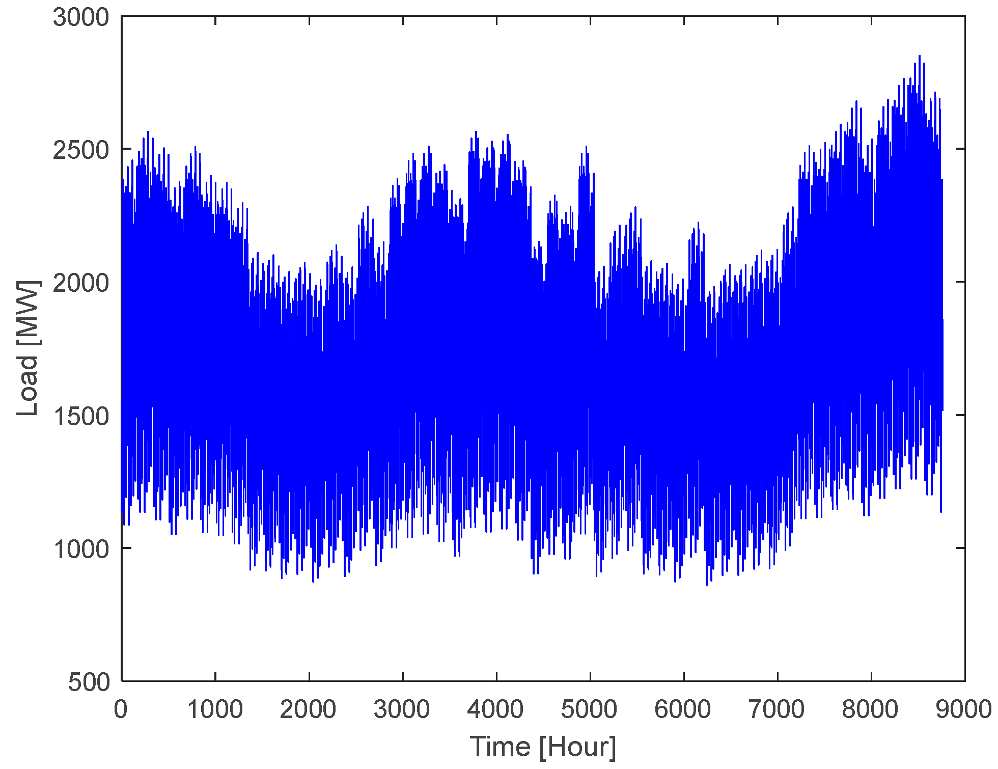
4. Case Study and Discussion

This section presents a comprehensive case study to assess the performance of various uncertainty modeling techniques in a power system integrating wind farms. The studied system is the IEEE 24-Bus reliability test system, which is affected by fluctuations in wind speeds and a reduction in the generation of conventional power plants (CPPs). Details of the system configuration and data processing are provided in [12,87].

First, two scenarios were considered for the levels of CPP generation reduction, combined with wind power variability. Next, reliability metrics were computed using probabilistic simulations. These simulations incorporated uncertainty modeling techniques to evaluate the system’s performance under uncertain wind conditions. Finally, the economic impact of energy not supplied was calculated to quantify the cost implications of reliability challenges in different scenarios.

This analysis compares the Monte Carlo simulation combined with the K-Means method, MCMC, RO, and IGDT in managing the uncertainty of wind farm generation over different time horizons. The number of Monte Carlo simulation scenarios is considered 300, the number of Markov chain states is considered 10, and the worst-case uncertainty level parameter for both IGDT and RO is considered 0.2. The cut-in wind speed, cut-out wind speed, and rated wind speed for wind turbines are considered 4 m/s, 20 m/s, and 16 m/s, respectively. The rated power of each wind turbine is 1 MW and the total number of wind turbines in the wind farm is 1000 (i.e., total capacity of wind farm is 1000 MW). This paper evaluates how uncertainty affects key reliability indices such as LOLE, LOLP, and EENS.

Due to the extensive nature of the data analyzed, spanning an entire year in some cases, presenting all individual data points numerically would be impractical. Therefore, key results are summarized in figures, which effectively highlight trends, relationships, and comparative performances across methods.

Real wind speed data were sourced from Milwaukee, USA, through Meteoblue’s weather archive [88], covering an entire year. This combination of the IEEE test system and real-world wind data ensures the analysis reflects practical and realistic conditions.

Figure 8 illustrates the annual system load profile, displaying fluctuations between 861 MW and 2850 MW. On the other hand, Figure 9 illustrates the generation output from 33 CPPs over the period of one year, fluctuating between 2624 MW and 4539 MW.

The generation of conventional power plants (CPPs) does not correlate with wind speed because CPPs are dispatchable and their output is determined by the consideration of grid demand, market conditions, and reliability requirements. In contrast, wind farm generation depends directly on wind speed. Wind farms contribute renewable energy when wind conditions are favorable, while CPPs provide stability and reliability to balance the grid during periods of low wind generation or high load.

Figure 10 presents the historical wind speed data over the period of one year. The wind speeds exhibit significant variability, ranging from near 0 to over 30 m/s, with occasional high spikes above 25 m/s.

Figure 11a,b compare wind speed data modeled by different uncertainty modeling techniques, including Monte Carlo simulation combined with the K-Means method, MCMC, IGDT, and RO, for the last month of the year and last 3 months of the year, respectively, alongside the actual historical data. Monte Carlo provides more conservative estimates in instances of normal wind speeds compared to historical data, while IGDT and RO provide estimates with fewer spikes for wind speeds compared to Monte Carlo simulation and MCMC methods.

Table 2. Comparison of the correlation between the results of different uncertainty modeling techniques (1-month uncertainty) with real historical data of wind speeds.

	Technique	Monte Carlo and K-Means		MCMC		IGDT		Robust
Index
Uncertainty duration [month]		1	3	1	3	1	3	1	3
Correlation coefficient between the wind speeds modeled by the uncertainty modeling technique and real historical data of wind speeds		0.9682	0.9748	0.9191	0.9711	0.9508	0.9578	0.9272	0.9381

provides a comparison of the correlation coefficients between the wind speeds modeled by various uncertainty modeling techniques and real historical wind speed data, calculated using the “corr2” function in MATLAB (version R2024a). This table focuses on both one-month and three-month uncertainty durations, allowing for an evaluation of how well each technique aligns with actual wind conditions. Monte Carlo simulation combined with the K-Means method demonstrates the highest correlation with real wind speed data, particularly over extended uncertainty periods. This result highlights the combined strengths of Monte Carlo’s robust coverage of uncertainty and K-Means’ ability to minimize intra-cluster distances. However, this finding reflects the specific metrics and conditions of the case study and should not be interpreted as a universal assertion of superiority in risk modeling. Other methods, such as Markov Chain Monte Carlo, IGDT, and robust optimization, have unique strengths depending on the application and context. MCMC improves over longer durations, while IGDT and robust optimization provide moderate accuracy. The increase in the correlation factor with longer time horizons can be attributed to the smoothing effect of aggregation. Longer time horizons average out these fluctuations, emphasizing the more stable and consistent relationship between wind speed and wind generation.

Table 3. Comparison of the system performance without the wind farm and with reductions of 20% and 30% in the generation of CPPs.

Index	20% Reduction in the Generation of CPPs	30% Reduction in the Generation of CPPs
LOLE [hours per year]	14.77	314.23
LOLP	0.00502	0.04646
EENS [MWh]	13.86	2423.14
EENS cost [USD]	4.85 × 104	8.48 × 106
Reliability	0.99969	0.99599

presents the system performance without wind farm integration, comparing the effects of a 20% and 30% reduction in the generation of CPPs. The results indicate that the absence of wind farms significantly impacts the system’s ability to maintain reliability, particularly as the reduction in CPP generation increases.

The relationship between EENS and its cost is a critical metric in power system reliability. EENS represents the energy demand not met by the generation system, and its cost is calculated using the Value of Lost Load (VoLL), which is assumed to be USD 3500/MWh in this study. As Table 3 shows, reductions in CPP generation lead to an increase in EENS and a corresponding rise in costs, demonstrating the economic impact of reduced reliability. Wind farm integration helps mitigate these effects by contributing renewable energy to meet demand, reducing both EENS and its associated costs.

In the 20% reduction scenario, the system’s reliability remains relatively high but starts to show signs of deterioration and vulnerability. The LOLE increases to 14.77 h per year, which is a significant jump compared to systems with wind farm integration (as seen in

Table 4. Comparison of the system performance with various uncertainty modeling techniques for modeling the uncertainty of wind farming (1-month uncertainty) and with the reductions of 20% and 30% in the generation of CPPs.

	Case	20% Reduction in the Generation of CPPs Replaced by 1000 MW (Rated Power) Wind Farm					30% Reduction in the Generation of CPPs Replaced by 1000 MW (Rated Power) Wind Farm
Index		Real Case (Without Uncertainty)	Monte Carlo and K-Means	MCMC	IGDT	Robust	Real Case (Without Uncertainty)	Monte Carlo and K-Means	MCMC	IGDT	Robust
LOLE [hours per year]		0.70	0.70	0.48	0.67	0.77	49.26	49.13	48.86	49.52	49.95
LOLP		0.00114	0.00114	0.00057	0.00102	0.00136	0.01027	0.00970	0.00913	0.01084	0.01221
EENS [MWh]		0.77	0.83	0.02	0.75	1.35	90.21	89.25	72.85	93.47	130.50
EENS cost [USD]		2.69 × 103	2.92 × 103	0.09 × 103	2.64 × 103	4.75 × 103	3.15 × 105	3.12 × 105	2.54 × 105	3.27 × 105	4.56 × 105
Reliability		0.99993	0.99992	0.99999	0.99993	0.99990	0.99920	0.99920	0.99933	0.99919	0.99897

and

Table 5. Comparison of the system performance with various uncertainty modeling techniques for modeling the uncertainty of wind farming (3-month uncertainty) and with reductions of 20% and 30% in the generation of CPPs.

	Case	20% Reduction in the Generation of CPPs Replaced by 1000 MW (Rated Power) Wind Farm					30% Reduction in the Generation of CPPs Replaced by 1000 MW (Rated Power) Wind Farm
Index		Real case (Without Uncertainty)	Monte Carlo and K-Means	MCMC	IGDT	Robust	Real case (Without Uncertainty)	Monte Carlo and K-Means	MCMC	IGDT	Robust
LOLE [hours per year]		0.70	0.70	0.29	0.81	0.84	49.26	49.18	48.92	50.13	49.45
LOLP		0.00114	0.00114	0.00057	0.00125	0.00159	0.01027	0.00958	0.00890	0.01073	0.01152
EENS [MWh]		0.77	0.85	0.07	0.94	1.59	90.21	87.90	66.38	105.88	122.57
EENS cost [USD]		2.69 × 103	2.98× 103	0.26 × 103	3.30 × 103	5.57 × 103	3.15 × 105	3.07 × 105	2.32 × 105	3.70 × 105	4.29 × 105
Reliability		0.99993	0.99992	0.99998	0.99992	0.99988	0.99920	0.99922	0.99940	0.99912	0.99898

). Similarly, the LOLP rises to 0.00502, indicating a noticeable increase in the probability of losing load. The EENS reaches 13.86 MWh, and the associated cost escalates to USD 4.85 × 10⁴, reflecting the system’s growing challenges in supplying energy without wind power as a backup.

In the 30% reduction scenario, the system experiences a dramatic decline in performance without wind farm integration. The LOLE spikes to 314.23 h per year, and the LOLP increases substantially to 0.04646, suggesting that the system is highly prone to frequent shortages. The EENS also increases significantly to 2423.14 MWh, with an associated cost of USD 8.48 × 10⁶, and the reliability drops to 0.99599, underscoring the severe energy shortfalls and the technical and financial implications of the reduced CPP generation without renewable energy support.

Table 4 evaluates system performance over a one-month period using various uncertainty modeling techniques, focusing on the impacts of 20% and 30% reductions in CPP generation. The real case, which excludes uncertainty, provides a baseline with key metrics like LOLE, LOLP, and EENS, along with EENS cost.

In the 20% reduction scenario, the real case shows a highly reliable system with an LOLE of 0.70 h, LOLP of 0.00114, and EENS of 0.77 MWh, with an associated cost of USD 2.69 × 10³. Monte Carlo simulation combined with K-Means closely matches the real case, with an EENS of 0.83 MWh and a cost of USD 2.92 × 10³. MCMC, however, underestimates vulnerability, predicting an LOLE of 0.48 h and EENS of just 0.02 MWh, with an associated cost of USD 0.09 × 10³.

In the 30% reduction scenario, the real case shows significant vulnerability, with an LOLE of 49.26 h and EENS of 90.21 MWh. Monte Carlo with K-Means performs well, showing an LOLE of 49.13 h and an EENS of 89.25 MWh. MCMC underestimates risks, while IGDT and robust optimization methods present more conservative estimates, with IGDT predicting an EENS of 93.47 MWh and the robust optimization method estimating 130.50 MWh, reflecting their cautious approach.

Table 5 extends the system performance evaluation over a three-month period. The real case shows a low LOLE of 0.70 h per year for the 20% reduction scenario and 49.26 h per year for the 30% reduction scenario. Monte Carlo simulation combined with K-Means closely follows the real case, while MCMC underestimates risks. IGDT and robust optimization methods provide more conservative estimates, particularly in the 30% reduction scenario, where they predict higher LOLE and EENS values.

While the numerical differences between methods may appear minor, they hold significant implications for power system reliability and operational decision-making. For example, Monte Carlo methods provide extensive uncertainty coverage, which is critical for systems requiring a comprehensive exploration of potential scenarios. IGDT, on the other hand, focuses on worst-case outcomes, making it particularly effective for risk-averse strategies. Sensitivity analyses demonstrate that these differences become more pronounced under conditions of high uncertainty, emphasizing the importance of selecting the appropriate method based on specific operational objectives.

Figure 12 illustrates the LOLP as a function of the percentage reduction in CPP generation without wind farm integration. The LOLP remains near zero for reductions up to 30–40%, indicating that the system can handle small reductions in CPP generation. However, beyond this threshold, the LOLP increases sharply, especially as reductions reach 50% or more. By the time CPP generation is reduced by 80–100%, the LOLP approaches 1, meaning that the likelihood of system failure or blackouts is nearly certain. This steep rise shows the system’s increasing vulnerability to loss of load as conventional generation decreases without wind energy to compensate.

Figure 13 depicts the LOLE as a function of CPP generation reduction, excluding wind farm integration. Like LOLP, the LOLE remains low for reductions up to 30–40%. However, beyond this point, the LOLE rises dramatically, indicating that the system becomes increasingly unable to meet load demand. When CPP generation reductions reach 70–80%, the LOLE approaches its maximum, representing thousands of expected hours of load loss per year. This shows the severe consequences of high CPP reductions on system performance.

Figure 14 shows the EENS as a function of CPP generation reduction, without wind farm contributions. The EENS remains low for up to a 30–40% reduction, suggesting that the system can manage small reductions in conventional generation. However, beyond the 40% threshold, the EENS rises sharply, exhibiting exponential growth as reductions increase. By the time CPP reductions reach 70–80%, the EENS approaches extremely high levels, meaning the system cannot meet a large portion of its energy demand. This exponential rise highlights the risk of significant energy shortfalls as conventional generation continues to decline.

Figure 15 illustrates system reliability as a function of CPP generation reduction, again without wind farm integration. As reductions in CPPs increase, reliability remains relatively stable only up to 30–40%. Beyond this threshold, reliability declines sharply, dropping steeply as reductions surpass 50%. By the time CPP generation reductions reach 80–100%, system reliability approaches zero, meaning the system is almost entirely unreliable. This sharp drop highlights the system’s critical dependence on conventional generation to maintain stability.

Figure 16 examines the impact of wind farm integration on the LOLP as CPP generation is reduced, comparing different uncertainty durations and modeling techniques. Both sub-figures exclude the real case to focus on how models handle wind and conventional power uncertainties.

Figure 16a, under a 1-month uncertainty scenario, shows the LOLP remaining low and stable for up to a 30–40% CPP generation reduction, with Monte Carlo and IGDT methods closely matching real-case performance. Beyond 40%, the LOLP rises steadily, though wind integration mitigates sharp increases. In Figure 16b, under a 3-month uncertainty, a similar trend is observed, but differences between models become more pronounced over time. IGDT and Monte Carlo continue to perform best, with the LOLP increasing more rapidly after a 40% reduction.

Compared to Figure 13 (without wind farms), wind farms significantly lower LOLP even as CPP generation decreases, highlighting wind’s role in reducing load loss risks.

Figure 17 explores the impact of wind farms on the LOLE under both 1-month and 3-month uncertainty scenarios. In Figure 17a, wind farms help maintain a low LOLE even as CPP generation decreases, with Monte Carlo and IGDT closely matching real-case performance. In Figure 17b, under a 3-month uncertainty, the LOLE rises more rapidly beyond a 40% CPP reduction. Again, Monte Carlo and IGDT deliver reliable predictions over extended periods.

Compared to Figure 13 (without wind farms), Figure 17 shows that wind farms significantly reduce the LOLE, particularly in longer uncertainty scenarios, proving their importance in enhancing reliability under reduced CPP generation.

Figure 18 assesses the EENS with wind farm integration. In Figure 18a, under 1-month uncertainty, the EENS stays stable up to a 30–40% CPP reduction but increases sharply beyond 50%. Monte Carlo and IGDT closely align with real-case results. In Figure 18b, under 3-month uncertainty, the EENS rises steeply after a 40% reduction, with Monte Carlo performing best over the longer horizon.

Figure 18 compared to Figure 14 (without wind farms) shows that wind farms mitigate the EENS, though their effectiveness lessens with longer uncertainty periods.

Figure 19 evaluates the overall system reliability with wind farm integration. In Figure 19a, under 1-month uncertainty, reliability remains high up to a 40% CPP reduction, with wind stabilizing the system. In Figure 19b, under 3-month uncertainty, reliability drops more after a 40% reduction, as wind’s impact lessens. Monte Carlo remains the most reliable for extended uncertainties.

Compared to Figure 15 (without wind farms), wind farms significantly boost reliability, especially in short-term scenarios, though their effect diminishes over longer periods.

The results underscore the pivotal role of integrating wind farms in enhancing the reliability of power systems, particularly when conventional power generation faces significant reductions. The Monte Carlo simulation coupled with K-Means proved to be the most effective in closely aligning with real-case scenarios and managing uncertainties across both short and longer durations. These findings highlight the necessity of adopting advanced modeling techniques to accurately predict and manage the dynamics of power systems with high renewable penetration. The successful application of these models demonstrates their potential in guiding energy policy and system design to ensure stability and reliability in the evolving energy landscape.

5. Conclusions

The integration of RESs into modern power systems has introduced new complexities, particularly due to the inherent variability and uncertainty in power generation. This paper reviews the state-of-the-art techniques for modeling uncertainty and risk in power systems. It covers a range of methodologies, including probabilistic, possibilistic, and robust optimization approaches, and provides a comparative analysis of their applicability in managing the variability in renewable energy sources like wind farms. The review also includes advanced techniques such as IGDT, RO, and Monte Carlo simulations, highlighting their role in enhancing power system reliability under uncertainty. Through the detailed analysis of case studies focusing on wind farming, the paper demonstrates how these techniques can be effectively applied to manage uncertainties in power generation. While the integration of wind turbines improves the system’s overall reliability when there are reductions in the generation of CPPs, the key factor is how closely the uncertainty models reflect real-world performance. Based on the results, Monte Carlo simulation combined with the K-Means method demonstrated strong performance in the case study, yielding the highest correlation with historical wind speed data. However, this outcome should be viewed within the context of the specific metrics and application used. The distinct principles of Monte Carlo and K-Means—coverage and distance minimization, respectively—contribute to this result but do not imply universal superiority. Other techniques, such as IGDT and robust optimization, provide complementary strengths and should be evaluated based on the specific needs and challenges of the power system under study. These techniques not only enhance the precision of risk modeling but also contribute to a better understanding of how decision-making frameworks can be adapted to modern power systems. In conclusion, ongoing research and development of these risk management strategies are essential for maintaining the stability and reliability of future power systems. As renewable energy penetration continues to rise, the application of these sophisticated models will be critical in ensuring the safe and efficient operation of power grids. Future research can expand the reliability and risk assessment techniques to areas like civil engineering and airborne systems, enhancing their robustness and applicability. However, challenges such as adapting methods to domain-specific uncertainties, incorporating real-time data, and managing computational complexity require interdisciplinary collaboration and innovative solutions.

References

1. Billinton, R.; Chu, K. Early evolution of LOLP: Evaluating generating capacity requirements [history]. IEEE Power Energy Mag. 2015, 13, 88–98. [Google Scholar] [CrossRef]
2. Skare, E.; Haugdal Jore, S. Hybrid threats in the Norwegian petroleum sector. A new category of risk problems for safety science? Saf. Sci. 2024, 176, 106521. [Google Scholar] [CrossRef]
3. Aven, T. A risk and safety science perspective on the precautionary principle. Saf. Sci. 2023, 165, 106211. [Google Scholar] [CrossRef]
4. Blokland, P.; Reniers, G. Safety Science, a Systems Thinking Perspective: From Events to Mental Models and Sustainable Safety. Sustainability 2020, 12, 5164. [Google Scholar] [CrossRef]
5. Chen, D.; Chen, J.D. Monte-Carlo Simulation-Based Statistical Modeling; Springer: Berlin/Heidelberg, Germany, 2017. [Google Scholar]
6. IEC 61400-26-1:2019; Wind Energy Generation Systems—Part 26-1: Availability for Wind Energy Generation Systems. Swedish Institute for Standards: Stockholm, Sweden, 2019.
7. Lutz, M.; Görg, P.; Faulstich, S.; Cernusko, R.; Pfaffel, S. Monetary-based availability: A novel approach to assess the performance of wind turbines. Wind Energy 2020, 23, 77–89. [Google Scholar] [CrossRef]
8. Shrestha, T.K.; Karki, R. Utilizing energy storage for operational adequacy of wind-integrated bulk power systems. Appl. Sci. 2020, 10, 5964. [Google Scholar] [CrossRef]
9. Wang, M.Q.; Yang, M.; Liu, Y.; Han, X.S.; Wu, Q. Optimizing probabilistic spinning reserve by an umbrella contingencies constrained unit commitment. Int. J. Electr. Power Energy Syst. 2019, 109, 187–197. [Google Scholar] [CrossRef]
10. Moghaddam, M.J.H.; Kalam, A.; Nowdeh, S.A.; Ahmadi, A.; Babanezhad, M.; Saha, S. Optimal sizing and energy management of stand-alone hybrid photovoltaic/wind system based on hydrogen storage considering LOEE and LOLE reliability indices using flower pollination algorithm. Renew. Energy 2019, 135, 1412–1434. [Google Scholar] [CrossRef]
11. Stephen, G.; Tindemans, S.H.; Fazio, J.; Dent, C.; Acevedo, A.F.; Bagen, B.; Crawford, A.; Klaube, A.; Logan, D.; Burke, D. Clarifying the interpretation and use of the LOLE resource adequacy metric. In Proceedings of the 2022 17th International Conference on Probabilistic Methods Applied to Power Systems (PMAPS), Manchester, UK, 15–12 June 2022; pp. 1–4. [Google Scholar]
12. Billinton, R.; Ronald, N.A. Reliability Evaluation of Power Systems; Springer Science & Business Media: Berlin, Germany, 2013. [Google Scholar]
13. Sun, D.; Zheng, Z.; Liu, S.; Wang, M.; Sun, Y.; Liu, D. Generation expansion planning considering efficient linear EENS formulation. Glob. Energy Interconnect. 2021, 4, 273–284. [Google Scholar] [CrossRef]
14. Bohre, A.K.; Agnihotri, G.; Dubey, M. Optimal sizing and sitting of DG with load models using soft computing techniques in practical distribution system. IET Gener. Transm. Distrib. 2016, 10, 2606–2621. [Google Scholar] [CrossRef]
15. Cui, Z.; Zheng, M.; Wang, J.; Liu, J. Reliability Analysis of a Three-Engine Simultaneous Pouring Control System Based on Bayesian Networks Combined with FMEA and FTA. Appl. Sci. 2023, 13, 11546. [Google Scholar] [CrossRef]
16. Andrews, J.; Tolo, S. Dynamic and dependent tree theory (D2T2): A framework for the analysis of fault trees with dependent basic events. Reliab. Eng. Syst. Saf. 2023, 230, 108959. [Google Scholar] [CrossRef]
17. Chen, M.; Cao, X.; Zhang, Z.; Yang, L.; Ma, D.; Li, M. Risk-averse stochastic scheduling of hydrogen-based flexible loads under 100% renewable energy scenario. Appl. Energy 2024, 370, 123569. [Google Scholar] [CrossRef]
18. Ghaffarinasab, N.; Çavuş, Ö.; Kara, B.Y. A mean-CVaR approach to the risk-averse single allocation hub location problem with flow-dependent economies of scale. Transp. Res. Part B Methodol. 2023, 167, 32–53. [Google Scholar] [CrossRef]
19. Schneider, I. Jakob Bernoulli, Ars conjectandi (1713). In Landmark Writings in Western Mathematics 1640–1940; Elsevier: Amsterdam, The Netherlands, 2005; pp. 88–104. [Google Scholar]
20. Gupta, A.K.; Varga, T. An Introduction to Actuarial Mathematics; Springer Science & Business Media: Amsterdam, The Netherlands, 2013. [Google Scholar]
21. Paltrinieri, N.; Comfort, L.; Reniers, G. Learning about risk: Machine learning for risk assessment. Saf. Sci. 2019, 118, 475–486. [Google Scholar] [CrossRef]
22. Esposito, S.; Stojadinovic, B.; Mignan, A.; Dolšek, M.; Babič, A.; Selva, J.; Iqbal, S.; Cotton, F.; Iervolino, I. Report on the Proposed Engineering Risk Assessment Methodology for Stress Tests of Non-Nuclear Cis; ETH: Zurich, Switzerland, 2016. [Google Scholar]
23. Quiles-Cucarella, E.; Marquina-Tajuelo, A.; Roldán-Blay, C.; Roldán-Porta, C. Particle Swarm Optimization Method for Stand-Alone Photovoltaic System Reliability and Cost Evaluation Based on Monte Carlo Simulation. Appl. Sci. 2023, 13, 11623. [Google Scholar] [CrossRef]
24. Reis, D.J.F.; Pessanha, J.E.O. A fast and accurate sampler built on Bayesian inference and optimized Hamiltonian Monte Carlo for voltage sag assessment in power systems. Int. J. Electr. Power Energy Syst. 2023, 153, 109297. [Google Scholar] [CrossRef]
25. Liu, C.; Zheng, X.; Yang, H.; Tang, W.; Sang, G.; Cui, H. Techno-economic evaluation of energy storage systems for concentrated solar power plants using the Monte Carlo method. Appl. Energy 2023, 352, 121983. [Google Scholar] [CrossRef]
26. Hassani, B.; Hassani, B.K. Scenario Analysis in Risk Management; Springer: Berlin/Heidelberg, Germany, 2016. [Google Scholar]
27. Chen, L.; Chen, C.; Wang, L.; Zeng, W.; Li, Z. Uncertainty quantification of once-through steam generator for nuclear steam supply system using latin hypercube sampling method. Nucl. Eng. Technol. 2023, 55, 2395–2406. [Google Scholar] [CrossRef]
28. Helton, J.C.; Davis, F.J. Latin hypercube sampling and the propagation of uncertainty in analyses of complex systems. Reliab. Eng. Syst. Saf. 2003, 81, 23–69. [Google Scholar] [CrossRef]
29. Cai, J.; Hao, L.; Xu, Q.; Zhang, K. Reliability assessment of renewable energy integrated power systems with an extendable Latin hypercube importance sampling method. Sustain. Energy Technol. Assess. 2022, 50, 101792. [Google Scholar] [CrossRef]
30. Bulut, E.; Albak, E.İ.; Sevilgen, G.; Öztürk, F. A new approach for battery thermal management system design based on Grey Relational Analysis and Latin Hypercube Sampling. Case Stud. Therm. Eng. 2021, 28, 101452. [Google Scholar] [CrossRef]
31. Hirsch, C.; Wunsch, D.; Szumbarski, J.; Łaniewski-Wołłk, L.; Pons-Prats, J. Uncertainty management for robust industrial design in aeronautics. In Notes on Numerical Fluid Mechanics and Multidisciplinary Design; Springer: Cham, Switzerland, 2019. [Google Scholar]
32. Liu, Y.; Wang, J.; Yue, Z. Improved Multi-point estimation method based probabilistic transient stability assessment for power system with wind power. Int. J. Electr. Power Energy Syst. 2022, 142, 108283. [Google Scholar] [CrossRef]
33. Pesteh, S.; Moayyed, H.; Miranda, V. Favorable properties of Interior Point Method and Generalized Correntropy in power system State Estimation. Electr. Power Syst. Res. 2020, 178, 106035. [Google Scholar] [CrossRef]
34. Kan, R.; Xu, Y.; Li, Z.; Lu, M. Calculation of probabilistic harmonic power flow based on improved three-point estimation method and maximum entropy as distributed generators access to distribution network. Electr. Power Syst. Res. 2024, 230, 110197. [Google Scholar] [CrossRef]
35. Aien, M.; Hajebrahimi, A.; Fotuhi-Firuzabad, M. A comprehensive review on uncertainty modeling techniques in power system studies. Renew. Sustain. Energy Rev. 2016, 57, 1077–1089. [Google Scholar] [CrossRef]
36. Calderaro, V.; Lamberti, F.; Galdi, V.; Piccolo, A. Power flow problems with nested information: An approach based on fuzzy numbers and possibility theory. Electr. Power Syst. Res. 2018, 158, 275–283. [Google Scholar] [CrossRef]
37. Mandal, S.; Maiti, J. Risk analysis using FMEA: Fuzzy similarity value and possibility theory based approach. Expert Syst. Appl. 2014, 41, 3527–3537. [Google Scholar] [CrossRef]
38. Murthy, C.; Varma, K.A.; Roy, D.S.; Mohanta, D.K. Mohanta Reliability Evaluation of Phasor Measurement Unit Using Type-2 Fuzzy Set Theory. IEEE Syst. J. 2014, 8, 1302–1309. [Google Scholar] [CrossRef]
39. Woo, T.H.; Jang, K.B.; Baek, C.H.; Choi, J.D. Analysis of climate change mitigations by nuclear energy using nonlinear fuzzy set theory. Nucl. Eng. Technol. 2022, 54, 4095–4101. [Google Scholar] [CrossRef]
40. Wang, J.; Xu, L.; Cai, J.; Fu, Y.; Bian, X. Offshore wind turbine selection with a novel multi-criteria decision-making method based on Dempster-Shafer evidence theory. Sustain. Energy Technol. Assess. 2022, 51, 101951. [Google Scholar] [CrossRef]
41. Tian, W.; de Wilde, P.; Li, Z.; Song, J.; Yin, B. Uncertainty and sensitivity analysis of energy assessment for office buildings based on Dempster-Shafer theory. Energy Convers. Manag. 2018, 174, 705–718. [Google Scholar] [CrossRef]
42. Sentz, K.; Ferson, S. Combination of Evidence in Dempster-Shafer Theory; Springer: Berlin/Heidelberg, Germany, 2002. [Google Scholar]
43. Wu, Y.; Chen, M.; Shen, K.; Wang, J. Z-number extension of TODIM-CPT method combined with K-means clustering for electric vehicle battery swapping station site selection. J. Energy Storage 2024, 85, 110900. [Google Scholar] [CrossRef]
44. Zhang, X.; Goh, M.; Bai, S.; Wang, Q. Green, resilient, and inclusive supplier selection using enhanced BWM-TOPSIS with scenario-varying Z-numbers and reversed PageRank. Inf. Sci. 2024, 674, 120728. [Google Scholar] [CrossRef]
45. Zadeh, L.A. A Note on Z-numbers. Inf. Sci. 2011, 181, 2923–2932. [Google Scholar] [CrossRef]
46. Zeng, B.; Wei, X.; Zhao, D.; Singh, C.; Zhang, J. Hybrid probabilistic-possibilistic approach for capacity credit evaluation of demand response considering both exogenous and endogenous uncertainties. Appl. Energy 2018, 229, 186–200. [Google Scholar] [CrossRef]
47. Khaloie, H.; Abdollahi, A.; Rashidinejad, M.; Siano, P. Risk-based probabilistic-possibilistic self-scheduling considering high-impact low-probability events uncertainty. Int. J. Electr. Power Energy Syst. 2019, 110, 598–612. [Google Scholar] [CrossRef]
48. Roukerd, S.P.; Abdollahi, A.; Rashidinejad, M. Probabilistic-possibilistic flexibility-based unit commitment with uncertain negawatt demand response resources considering Z-number method. Int. J. Electr. Power Energy Syst. 2019, 113, 71–89. [Google Scholar] [CrossRef]
49. Maulik, A. A hybrid probabilistic information gap decision theory based energy management of an active distribution network. Sustain. Energy Technol. Assess. 2022, 53, 102756. [Google Scholar] [CrossRef]
50. Yarmohammadi, H.; Abdi, H. Optimal operation of multi-carrier energy systems considering demand response: A hybrid scenario-based/IGDT uncertainty method. Electr. Power Syst. Res. 2024, 235, 110877. [Google Scholar] [CrossRef]
51. Li, J.; Yu, Z.; Mu, G.; Li, B.; Zhou, J.; Yan, G.; Zhu, X.; Li, C. An assessment methodology for the flexibility capacity of new power system based on two-stage robust optimization. Appl. Energy 2024, 376, 124291. [Google Scholar] [CrossRef]
52. Zhang, C.; Li, Y.; Zhang, H.; Wang, Y.; Huang, Y.; Xu, J. Distributionally robust resilience optimization of post-disaster power system considering multiple uncertainties. Reliab. Eng. Syst. Saf. 2024, 251, 110367. [Google Scholar] [CrossRef]
53. Wang, H.; Yi, Z.; Xu, Y.; Cai, Q.; Li, Z.; Wang, H.; Bai, X. Data-driven distributionally robust optimization approach for the coordinated dispatching of the power system considering the correlation of wind power. Electr. Power Syst. Res. 2024, 230, 110224. [Google Scholar] [CrossRef]
54. Dai, J.; Ding, C.; Yan, C.; Tang, Y.; Zhou, X.; Xue, F. Robust optimization method of power system multi resource reserve allocation considering wind power frequency regulation potential. Int. J. Electr. Power Energy Syst. 2024, 155, 109599. [Google Scholar] [CrossRef]
55. Li, Z.; Liu, M.; Xie, M.; Zhu, J. Robust optimization approach with acceleration strategies to aggregate an active distribution system as a virtual power plant. Int. J. Electr. Power Energy Syst. 2022, 142, 108316. [Google Scholar] [CrossRef]
56. Kang, J.; Wu, Z.; Ng, T.S.; Su, B. A stochastic-robust optimization model for inter-regional power system planning. Eur. J. Oper. Res. 2023, 310, 1234–1248. [Google Scholar] [CrossRef]
57. Ben-Tal, A.; El Ghaoui, L.; Nemirovski, A. Robust Optimization; Princeton University Press: Princeton, NJ, USA, 2009. [Google Scholar]
58. Sasaki, Y.; Takahashi, N.; Zoka, Y.; Yorino, N.; Bedawy, A.; Krifa, C.; Sekizkai, S. Day-ahead Generation Scheduling with Information Gap Decision Models. IFAC-Pap. 2024, 58, 152–157. [Google Scholar] [CrossRef]
59. Seyyedeh-Barhagh, S.; Abapour, M.; Mohammadi-Ivatloo, B.; Shafie-khah, M. Risk-based Peer-to-peer Energy Trading with Info-Gap Approach in the Presence of Electric Vehicles. Sustain. Cities Soc. 2023, 99, 104948. [Google Scholar] [CrossRef]
60. Fathi, R.; Tousi, B.; Galvani, S. A new approach for optimal allocation of photovoltaic and wind clean energy resources in distribution networks with reconfiguration considering uncertainty based on info-gap decision theory with risk aversion strategy. J. Clean. Prod. 2021, 295, 125984. [Google Scholar] [CrossRef]
61. Ben-Haim, Y. Feedback for energy conservation: An info-gap approach. Energy 2021, 223, 119957. [Google Scholar] [CrossRef]
62. Nojavan, S.; Zare, K.; Feyzi, M.R. Optimal bidding strategy of generation station in power market using information gap decision theory (IGDT). Electr. Power Syst. Res. 2013, 96, 56–63. [Google Scholar] [CrossRef]
63. Huang, D. Network reliability of a stochastic flow network by wrapping linear programming models into a Monte-Carlo simulation. Reliab. Eng. Syst. Saf. 2024, 252, 110427. [Google Scholar] [CrossRef]
64. Karki, R.; Hu, P.; Billinton, R. Reliability evaluation considering wind and hydro power coordination. IEEE Trans. Power Syst. 2009, 25, 685–693. [Google Scholar] [CrossRef]
65. Wu, L.; Shahidehpour, M.; Fu, Y. Security-constrained generation and transmission outage scheduling with uncertainties. IEEE Trans. Power Syst. 2010, 25, 1674–1685. [Google Scholar]
66. Ge, H.; Asgarpoor, S. Reliability evaluation of equipment and substations with fuzzy Markov processes. IEEE Trans. Power Syst. 2010, 25, 1319–1328. [Google Scholar]
67. Papavasiliou, A.; Oren, S.S.; O’Neill, R.P. Reserve requirements for wind power integration: A scenario-based stochastic programming framework. IEEE Trans. Power Syst. 2011, 26, 2197–2206. [Google Scholar] [CrossRef]
68. Odat, A.A.; Shawaqfah, M.; Al-Momani, F.; Shboul, B. Data of simulation model for photovoltaic system’s maximum power point tracking using sequential Monte Carlo algorithm. Data Brief 2024, 52, 109853. [Google Scholar] [CrossRef] [PubMed]
69. Venkatesh, B.; Yu, P.; Gooi, H.B.; Choling, D. Fuzzy MILP unit commitment incorporating wind generators. IEEE Trans. Power Syst. 2008, 23, 1738–1746. [Google Scholar] [CrossRef]
70. Zhang, X.; Pirouzi, A. Flexible energy management of storage-based renewable energy hubs in the electricity and heating networks according to point estimate method. Energy Rep. 2024, 11, 1627–1641. [Google Scholar] [CrossRef]
71. Liu, Z.; Wen, F.; Ledwich, G. Optimal siting and sizing of distributed generators in distribution systems considering uncertainties. IEEE Trans. Power Del. 2011, 26, 2541–2551. [Google Scholar] [CrossRef]
72. Lojowska, A.; Kurowicka, D.; Papaefthymiou, G.; Van Der Sluis, L. Stochastic modeling of power demand due to EVs using copula. IEEE Trans. Power Syst. 2012, 27, 1960–1968. [Google Scholar] [CrossRef]
73. Pantos, M. Exploitation of electric-drive vehicles in electricity markets. IEEE Trans. Power Syst. 2011, 27, 682–694. [Google Scholar] [CrossRef]
74. El-Khattam, W.; Hegazy, Y.G.; Salama, M. Investigating distributed generation systems performance using Monte Carlo simulation. IEEE Trans. Power Syst. 2006, 21, 524–532. [Google Scholar] [CrossRef]
75. Su, C. Stochastic evaluation of voltages in distribution networks with distributed generation using detailed distribution operation models. IEEE Trans. Power Syst. 2009, 25, 786–795. [Google Scholar] [CrossRef]
76. Zhang, H.; Li, P. Probabilistic analysis for optimal power flow under uncertainty. IET Gener. Transm. Distrib. 2010, 4, 553–561. [Google Scholar] [CrossRef]
77. Li, X.; Li, Y.; Zhang, S. Analysis of probabilistic optimal power flow taking account of the variation of load power. IEEE Trans. Power Syst. 2008, 23, 992–999. [Google Scholar]
78. Kazerooni, A.K.; Mutale, J. Transmission network planning under security and environmental constraints. IEEE Trans. Power Syst. 2010, 25, 1169–1178. [Google Scholar] [CrossRef]
79. Yamin, H.Y. Fuzzy self-scheduling for GenCos. IEEE Trans. Power Syst. 2005, 20, 503–505. [Google Scholar] [CrossRef]
80. Attaviriyanupap, P.; Kita, H.; Tanaka, E.; Hasegawa, J. A fuzzy-optimization approach to dynamic economic dispatch considering uncertainties. IEEE Trans. Power Syst. 2004, 19, 1299–1307. [Google Scholar] [CrossRef]
81. Singh, R.; Pal, B.C.; Vinter, R.B. Measurement placement in distribution system state estimation. IEEE Trans. Power Syst. 2009, 24, 668–675. [Google Scholar] [CrossRef]
82. Saric, A.T.; Ciric, R.M. Integrated fuzzy state estimation and load flow analysis in distribution networks. IEEE Trans. Power Del. 2003, 18, 571–578. [Google Scholar] [CrossRef]
83. Wang, Y.; Li, W.; Zhang, P.; Wang, B.; Lu, J. Reliability analysis of phasor measurement unit considering data uncertainty. IEEE Trans. Power Syst. 2012, 27, 1503–1510. [Google Scholar] [CrossRef]
84. Caro, E.; Morales, J.M.; Conejo, A.J.; Minguez, R. Calculation of measurement correlations using point estimate. IEEE Trans. Power Del. 2010, 25, 2095–2103. [Google Scholar] [CrossRef]
85. Perninge, M.; Lindskog, F.; Soder, L. Importance sampling of injected powers for electric power system security analysis. IEEE Trans. Power Syst. 2011, 27, 3–11. [Google Scholar] [CrossRef]
86. Duenas, P.; Reneses, J.; Barquin, J. Dealing with multi-factor uncertainty in electricity markets by combining Monte Carlo simulation with spatial interpolation techniques. IET Gener. Transm. Distrib. 2011, 5, 323–331. [Google Scholar] [CrossRef]
87. IEEE 24-Bus RTS. Available online: https://matpower.org/docs/ref/matpower5.0/case24_ieee_rts.html (accessed on 3 December 2024).
88. Meteoblue. Weather History Download Milwaukee. Available online: https://www.meteoblue.com/en/weather/archive/export/milwaukee_united-states-of%20america_5263045 (accessed on 3 December 2024).
Figure 1. Overview of risk modeling techniques.
Applsci 14 12042 g001
Figure 2. Conditional value-at-risk.
Applsci 14 12042 g002
Figure 3. Timeline of uncertainty modeling techniques.
Applsci 14 12042 g003
Figure 4. Various uncertainty modeling techniques.
Applsci 14 12042 g004
Figure 5. Fuzzy trapezoidal membership function.
Applsci 14 12042 g005
Figure 6. Z-number with the membership function μ A within the probability density function p X .
Applsci 14 12042 g006
Figure 7. Comparison of traditional optimization and RO.
Applsci 14 12042 g007
Figure 8. The system load for one year [9].
Applsci 14 12042 g008
Figure 9. CPPs’ generation for one year [9].
Applsci 14 12042 g009
Figure 10. Wind speeds’ historical data for one year.
Applsci 14 12042 g010
Figure 11. Wind speeds modeled by different uncertainty modeling techniques. (a) Wind speeds modeled for the last month of the year. (b) Wind speeds modeled for the last 3 months of the year.
Applsci 14 12042 g011
Figure 12. LOLP without wind farms and with the variation in the reduction in the CPPs’ generation.
Applsci 14 12042 g012
Figure 13. LOLE without wind farms and with the variation in the reduction in the CPPs’ generation.
Applsci 14 12042 g013
Figure 14. EENS without wind farms and with the variation in the reduction in the CPPs’ generation.
Applsci 14 12042 g014
Figure 15. Reliability without wind farms and with the variation in the reduction in the CPPs’ generation.
Applsci 14 12042 g015
Figure 16. LOLP with wind farms and the variation in the reduction in the CPPs’ generation. (a) One-month uncertainty (excluding real case). (b) Three-month uncertainty (excluding real case).
Applsci 14 12042 g016
Figure 17. LOLE with wind farms and the variation in the reduction in the CPPs’ generation. (a) One-month uncertainty (excluding real case). (b) Three-month uncertainty (excluding real case).
Applsci 14 12042 g017
Figure 18. EENS with wind farms and the variation in the reduction in the CPPs’ generation. (a) One-month uncertainty (excluding real case). (b) Three-month uncertainty (excluding real case).
Applsci 14 12042 g018
Figure 19. Reliability with wind farms and the variation in the reduction in the CPPs’ generation. (a) One-month uncertainty (excluding real case). (b) Three-month uncertainty (excluding real case).
Applsci 14 12042 g019