Abstract
The proliferation of uncategorized information on the Internet has intensified the need for effective recommender systems. Recommender systems have evolved from content-based filtering to collaborative filtering and, most recently, to deep learning-based and hybrid models. However, they often face challenges such as high computational costs, reduced reliability, and the Cold Start problem. We introduce a persona-based user modeling approach for real-time movie recommendations. Our system employs Non-negative Matrix Factorization (NMF) and Deep Learning algorithms to manage complex and sparse data types and to mitigate the Cold Start issue. Experimental results, based on criteria involving 50 topics and 35 personas, indicate a significant performance gain. Specifically, with 500 users, the precision@K for NMF was 86.01%, and for the Deep Neural Network (DNN), it was 92.67%. Tested with 900 users, the precision@K for NMF increased to 97.04%, and for DNN, it was 95.55%. These results represent an approximate 10% and 5% improvement in performance, respectively. The system not only delivers fast and accurate recommendations but also reduces computational overhead by updating the model only when user personas change. The generated user personas can be adapted for other recommendation services or large-scale data mining.
1. Introduction
Recommender systems typically analyze user ratings and choice histories to provide tailored suggestions. Recommendation algorithms include content-based filtering, collaborative filtering, deep learning, and hybrid recommendation techniques.
Content-based recommendation techniques analyze the properties of an item and recommend similar items. They recommend content similar to the items that users have used, preferred, or selected in the past. For example, in the context of movie recommendations, similar films are recommended to the user based on the genre, director, and actors of the movies that the user selected in the past. Content-based recommender systems directly reflect individual preferences. However, a drawback is that the accuracy of recommendations may decline in the absence of sufficient information about new items, or if the user lacks a diverse range of past experiences.
On the other hand, collaborative filtering recommendation techniques are based on the choices of other users who have similar preferences to the user. These techniques fundamentally ground their recommendations in measures of user similarity. Specifically, user-based collaborative filtering employs user similarity metrics to generate recommendations, while item-based collaborative filtering relies on item similarity for the same purpose. Deep learning-based recommendation techniques employ deep learning models of neural networks, to predict interactions between users and items for the purpose of making recommendations. Lastly, hybrid recommendation techniques combine the above recommendation methods to offset the limitations inherent in each individual recommender system.
Figure 1 illustrates the process of recommending movies with a conventional recommender system. After categorizing the features of each user’s favored movies, the recommender system computes similarities based on users’ rating matrices.
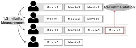
Figure 1.
Existing Recommender System—The process of Existing recommending movies with a conventional recommender system.
For example, in Figure 1, Users 1 and 3 have high user similarity. Therefore, the other movie that User 3 favored are recommended to User 1. When a new user appears, the similarities between the existing users and the new are measured for the recommendation to the new user.
Pearson correlation coefficient and the Cosine similarity are often used to measure such similarities. The Pearson correlation coefficient is a numerical measure indicating the relationship between two compared variables. It is used based on the ratings of items commonly rated by two users, with its formula being as follows:
Here, X and Y represent the ratings of the main user, and are the average ratings of other users, with +1 indicating a positive linear relationship, 0 indicating no linear relationship, and −1 indicating a negative linear relationship. The cosine similarity for two users is defined by the cosine of the angle between two vectors of users, and the formula is,
Here, X and Y represent the rating vectors of two users. The cosine similarity is between −1 and 1, where −1 indicates a completely different direction (i.e., an angle of 180 degrees), 1 indicates the same direction, and 0 corresponds to an angle of 90 degrees. The closer the cosine similarity value is to 1, the higher the similarity is judged to be.
Existing recommendation algorithms have to repeat similar calculations for new and rapidly created information (user or movie) using the Pearson correlation coefficient and Cosine similarity. The reason for repeatedly calculating the similarity for new users is to compare the preferences of the new users with those of the existing users to optimally recommend. This enables fast recommendations difficult due to the time and resources consumed by the iterative calculations required to compare the preferences of new users or items with those of existing users [1]. The need to calculate user similarities for a recommender system to reflect user preferences and provide personalized recommendations contributes to this issue. Such similarity calculations are time and resource-intensive tasks, with computational complexity increasing as the number of users or items increases. The need to recalculate these similarities each time a new user or item is added results in increased data storage and learning and computation time [2].
However, the existing techniques has several challenges. First, as the size of the computational matrix expands, computational time quickly grows. This makes it difficult to quickly make recommendations based on new data and results in increased costs. Second, the lack of initial interactions between users and items results in the sparsity, leading to decreased accuracy in recommendations. Third, the Cold Start emerges when new users or items are added to the recommender system. This problem results from the lack of initial information about users or items, making it difficult to make recommendations. Lastly, it is difficult to generate recommendations for inactive users or those not previously included in the recommender system.
This study proposes a user persona-based recommendation technique to address these issues. The user persona-based technique was developed to clearly understand and explain users’ goals and behavioral patterns [3]. A persona is a virtual character that consumes items and represents actual users, reflecting their characteristics. This technique helps to understand the target user and design products or services that suit that user from a user-centric perspective.
The recommender system implemented in this study used the movie rating data in MovieLens [4]. The ratings written by users were topic modeled through Latent Dirichlet Allocation (LDA). Then, each user was assigned topics, and these topics were clustered using K-Means Clustering to complete the final user Persona. Collaborative filtering (CF) is divided into memory-based CF and model-based CF [5]. Memory-based CF calculates the similarity of surrounding users to predict ratings. When the ratings data evaluated by the user is small compared to the total ratings data, the number of common evaluation items among users decreases. This makes it difficult to accurately calculate the similarity between users, leading to a decline in the accuracy of recommendations. Additionally, when new users or rating information is registered in the recommender system, situations in which there are few or no common evaluation items occur. Finally, when there are a small number of common evaluation items among users, the task of calculating the similarity between all users is very inefficient, and the complexity of calculations increases as the number of users and items increases with system expansion. These negatively affect the performances when there are few common evaluation items among users [6].
To overcome the lack of common evaluation items, we used the Non-negative Matrix Factorization (NMF), a model-based Collaborative Filtering (CF) method. NMF works by decomposing the rating matrix into two lower-dimension submatrices and then recombining them to predict missing ratings. Furthermore, we implemented our recommendation algorithm using a Deep Learning algorithm, one of the machine learning algorithms known for its outstanding performance. This method uses a multi-layer artificial neural network to simultaneously perform feature extraction and recommendation modeling. It learns the information of interactions between the user and the item, thereby providing accurate recommendations. We compared the movie recommendation information using the recommender system implemented through these two methods. The results showed that the system using the Deep Learning algorithm demonstrated a higher accuracy and performance [Table 1].

Table 1.
Comparison between NMF and Deep Learning Recommender Systems.
The NMF recommendation algorithm works by extracting latent factors from the user and item matrix. It represents each user and item as an n-dimensional vector and factorizes it into two lower-dimensional vectors. This factorization allows each element of the given user-item matrix to be represented as the dot product of the user vector and the item vector. These factorized vectors are used to recommend new items or analyze user preferences [7]. The NMF method is especially effective when there are few features or factors within the user-item matrix. Furthermore, NMF can be easily updated even when new items or users are added, without recalculating the existing data since it extracts latent factors within the data. NMF has a constraint that the factorized matrices are non-negative (0 or above). This prevents predicting user-item preferences below 0, providing more accurate recommendations. Secondly, NMF shows that the factorized matrices represent the latent features of users and items. This allows easy interpretation of what each feature means, enhancing the performance of the recommender system and increasing understanding of user-item interaction. Lastly, it reduces the dimensionality of the data. Since NMF factorizes into a low-rank matrix, it reduces the original high-dimensional data to a lower dimension. This simplifies complex data for faster processing during analysis.
Recommender systems using Deep Learning have various features. Firstly, they can utilize not only rating data but also various other data types. Conventional recommender systems primarily used item rating data evaluated by the user. However, recommender systems using Deep Learning can use not only rating data but also various data such as click history, search history, purchase history, review content, and activities on social media. Secondly, they can be used when the data contains many abstract and complex features such as the movie’s genre, director, and actors, which are difficult to express in simple numbers or categorical data in a movie recommender system. Deep Learning can easily learn such abstract information. Thirdly, recommender systems using Deep Learning can provide more precise recommendations using various information about users and items. For example, it can recommend movies based on the information about the user’s preferred genre, actors, and directors.
In programs that do not apply topic modeling and personas, the approximate recommendation time is about 10 s with an accuracy of 10%. However, with our modeling, the time is reduced to about 3 s, and the accuracy increases by 40%. Additionally, our model enables responsive movie recommendations based on changes in user personas.
All in all, recommender systems using Deep Learning can use more diverse data, easily learn data with abstract and complex features, and provide more precise and better recommendations, compared to traditional recommender systems.
2. Materials and Methods
2.1. Theoretical Backgrou
2.1.1. Recommender System
A recommender system is a technology that collects user data, understands individual preferences based on user preferences and past behavior, and recommends and provides suitable items. Types of recommender systems include content-based recommendations, which recommend similar items to those that the user has previously experienced, and collaborative recommendations, which measure similarity between users and recommend items that other users with similar preferences have rated [8]. Furthermore, there is the hybrid recommender system [Figure 2], which combines the advantages of content-based and collaborative recommendations.
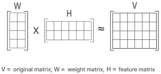
Figure 2.
Non-negative Matrix Factorization (NMF). NMF decomposes the entire matrix V into W and H.
Content-based filtering recommends items similar to the user’s preferences based on item characteristics or classification information. Collaborative filtering calculates similarity with other users based on user ratings or purchase history and makes recommendations. Hybrid filtering combines collaborative filtering and content-based filtering for recommendations [9]. Recently, recommender systems using deep learning algorithms have been widely studied. Notable examples of deep learning recommender systems include Neural Collaborative Filtering, a synthesis of the Multi-Layer Perceptron and Collaborative Filter, and the YouTube Recommendation [10], which divides the model into candidate models and ranking models for recommendations [10,11]. Deep learning has the ability to discover abstract and complex patterns from various data, and can use this ability to understand user preferences or item features more precisely and make recommendations. For example, deep learning is suitable for a movie recommender system to accurately identify user preferences using movie keywords, actors, and director information, and recommend similar movies. The recommender system analyzes the data collected through interaction between users and items to provide personalized recommendations, benefiting both users and item providers. Users can easily access complex product information and quickly find the items they want, and item providers can increase sales and improve customer satisfaction [12].
2.1.2. Algorithm-Based and Deep Learning Recommender Systems
We divide recommendation algorithms into algorithm-based recommender systems and deep learning-based recommender systems.
- -
- Algorithm-based Recommender Systems
Representative recommender systems include collaborative filtering, content-based filtering, hybrid filtering, etc. Open-source libraries implemented with matrix factorization, a way of implementing collaborative filtering, are available. However, there are three main issues with using such methods to build real-time personalized recommender systems [13]. First, memory usage increases sharply, and the learning speed slows down as the amount of training data increases. Second, user information is utilized not just as a single value of ID but in various ways. The accuracy is high when there exists a large database of user evaluation history, but there is a limitation in utilizing diverse user information. Lastly, it is difficult to implement quick recommendations in real time.
- -
- Deep learning-based Recommender Systems
The advantage of deep learning-based recommender systems is their ability to learn nonlinear and complex relationships among various features (e.g., user, item). While conventional methods focus on the linear relationships between users and items, deep learning uses nonlinear activation functions such as ReLU or Tanh, allowing it to represent nonlinear interactions and model complex relationships among various features. It effectively performs sophisticated inference by capturing various characteristics and interactions of the data, thus learning nonlinear patterns and demonstrating superior performance in various fields. Deep learning is receiving attention in various fields such as computer vision, speech recognition, and natural language processing due to its flexibility and powerful representational capability, contributing significantly to providing innovative solutions. Additionally, deep learning models have a modular expansion structure, ensuring exceptional scalability and flexibility. This implies that they may be combined with and replaced by other models. For instance, various factors such as a user’s past behavior, personal characteristics of the user, and the characteristics of items must be considered in recommender systems. The entire system can effectively handle various elements by choosing the deep learning module most suitable for modeling each of these elements and combining them.
For example, Recurrent Neural Networks (RNN) may be effective in modeling a user’s past behavior. At the same time, a Multilayer Perceptron (MLP) can model personal characteristics of the user, and a Convolutional Neural Network (CNN) can be useful for modeling the characteristics of items. By selecting and combining each of these modules, the entire system can effectively handle each element while maintaining flexibility.
Deep learning-based recommender systems can easily change to new deep learning models. In other words, the existing modules can be easily replaced with new ones when new models appear. This ensures that the recommender system always utilizes the latest technology to provide the best performance. A suitable form of deep learning models can be used to construct a recommender system depending on the form of the data.
2.1.3. Non-Negative Matrix Factorization (NMF)
NMF is based on the idea that humans recognize objects by combining parts of the object’s information, representing object information as features and semantic variables [7]. A piece of object information is factorized into two-part information composed of non-negative values. The purpose of NMF is to reduce object information by capturing only common features. It efficiently represents a large amount of information by representing the entire object through a combination of such part information. The NMF process involves finding the non-negative matrix factor W and H for the non-negative matrix V [7].
Non-negative Matrix Factorization (NMF) factorizes the original matrix into the product of two lower-dimensional matrices:
V ≈ WH
Here, V is the original data matrix, and W and H are the two matrices resulting from the factorization. All elements of these matrices are non-negative.
- Initialize two matrices, W and H, with the same size as the original matrix V and all elements being non-negative.
The size of W is set to [m, r] and H to [r, n]. Here, r is a given hyperparameter and is generally equal to or smaller than the number of columns in the original matrix.
- 2.
- Update W and H iteratively. For each update step, first fix W and update H, then fix H and update W. These updates are carried out in a direction that minimizes the difference between the original matrix V and the product of matrices W and H.
- 3.
- Continue this process until a certain number of iterations are reached, or the product of W and H becomes sufficiently close to V. The method of updating H is as follows:
H <- H .* ((W’ * V) ./(W’ * W * H + epsilon))
Here, ‘.*’ represents element-wise multiplication, and ‘./’ represents element-wise division. Epsilon is a very small constant to prevent division by zero.
The method of updating W is as follows:
W <- W .* ((V * H’) ./(W * H * H’ + epsilon))
Through this process, matrices W and H that are very close to the original matrix V can be obtained. Here, each column of W forms a basis representing features of the original data, and each row of H represents coefficients for the basis. NMF is used in this way to extract the structure of the original data and is utilized in various fields such as image analysis, text mining, and audio signal processing.
The “<-” symbol is used to signify the assignment of updated values to the matrices H and W, indicating the replacement of their current values with newly computed ones. The apostrophe in “H’” denotes the matrix H prior to its update.
- 4.
- Once the updates are completed, the product of W and H approximates the original matrix V. Here, W represents the ‘basis vectors’, and H represents the ‘weights’ of these vectors. The two constructed matrices can well represent the patterns of the original matrix.
- 5.
- In this way, NMF factorizes the structure of the original matrix into two smaller matrices, understanding the pattern of the data, and performs tasks such as prediction and classification based on this.
Thus, NMF is useful in extracting meaningful structures from original data. Under the condition that all elements of the original matrix are non-negative, NMF has the advantage of reflecting ‘part’ information well. This is especially useful in cases where each pixel or word in data like images or text independently has meaning. Also, unlike other dimension reduction techniques in machine learning and data analysis, NMF has the advantage of ease of interpretation, given that the resulting matrices are non-negative. Due to these features, NMF is used in various fields such as image recognition, text mining, gene expression pattern analysis. The goal of NMF is to minimize the error function. The formula is:
minimize ||V − WH||2
Here, ||•||2 denotes the Frobenius norm, which is the square root of the sum of the squares of each element of a matrix. The goal of NMF is to find W and H that minimize this error function. Optimization methods such as gradient descent or coordinate descent are typically used. These methods start by selecting initial values for W and H at random and then adjust W and H in the direction that reduces the error function. This process is repeated to find the optimal W and H.
2.1.4. Topic Modeling
Topic modeling is an analytical technique used to discover topics (abstract themes) in a document set. Although one could read a large number of documents and identify their topics, this requires significant time and effort. Topic modeling allows for the identification of topics by analyzing the simultaneous usage patterns of keywords in the text data, thereby automatically extracting the topics, issues, or topic groups that represent the documents. [Figure 3] illustrates typical topic modeling, which is composed of words, topics, and documents. Firstly, words represent the words appearing in each document. Topics are composed of words and the value of their influence in forming the topic. Finally, documents refer to a set of documents subject to topic modeling.
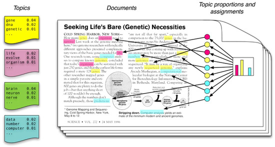
Figure 3.
Topic Modeling [14]—‘Seeking life’s bare (genetics) necessities’ refers to data analysis aimed at determining the number of genes necessary for an organism to survive within the framework of evolution. The words marked in blue, such as ‘computer’ and ‘prediction’, relate to data analysis. Those marked in pink, like ‘life’ and ‘organism’, pertain to evolutionary biology. The terms highlighted in yellow, ‘sequenced’ and ‘genes’, are associated with genetics.
Latent Dirichlet Allocation (LDA) demonstrates the probability of a specific word appearing in a specific topic. As shown in Figure 3, a document contains various topics. The words in the document are not formed from a specific theme but extracted from the topics represented by yellow, pink, and blue. There are multiple topics in a document. From these topics, we can determine which words were primarily used. Based on this, we can estimate the extent to which topics are included in a document. Each topic is a distribution of words. Thus, in the case of the yellow topic, the probability of the word “gene” appearing is 0.04, “dnas” is 0.02, and “genetic” is 0.01. This suggests that the topic marked with yellow is likely to be related with genetics. By looking at the entire document and the values of each topic, we can see that there are more words corresponding to the yellow topic than those corresponding to the pink and blue topics. From this, we can infer that the main topic of the document is related to genetics represented by the yellow topic.
Topic modeling is divided into matrix factorization-based methods and probability-based methods. The matrix factorization-based methods apply mathematical techniques like singular value factorization to large matrices containing statistical information from the corpus, such as word frequency, to reduce the dimensions of vectors in the matrix. Meanwhile, probability-based methods estimate the probability of a word existing in a specific topic and a specific topic existing in a document. Latent Semantic Analysis (LSA), based on Singular Value Factorization (SVD), is an example of matrix factorization-based topic modeling, while LDA is an example of the latter probability-based topic modeling.
2.1.5. Latent Dirichlet Analysis (LDA)
LDA is a widely used algorithm in topic modeling related to natural language processing. It estimates the combined probability of a word existing in a specific topic and a specific topic existing in a document, aiming to reveal significant topics. LDA is one of the probabilistic models for automatically extracting topics from a document set. LDA assumes that each document is composed of a mixture of various topics, and each topic is represented as a probability distribution of words. Figure 4 illustrates the process of assigning topics to each document and word, which is the ultimate goal of LDA. We need to pre-input the hyperparameters: (1) word distribution of topics (β), (2) topic distribution of documents (θ), and (3) the number of topics (k). Based on these inputs, we observe words (w) and assign appropriate topic numbers (z) to each word. The model iterates, updating the θ, β values, and finds the highest z-value to infer where each word in the document belongs [10]
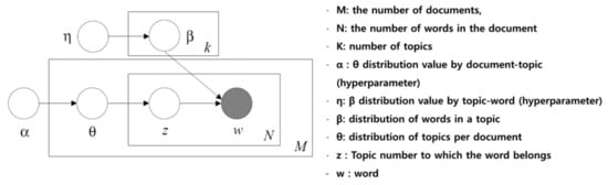
Figure 4.
Topic LDA—The LDA model graphically represented with plate notation.
2.1.6. Latent Semantic Analysis (LSA)
LSA is one of the topic modeling techniques used in natural language processing. It is an information retrieval technique for extracting the semantic content of a large text document and calculating the similarity between documents. LSA creates a word-document matrix and reducing it to a low-dimensional semantic space. It represents a given document set as a matrix and uses Singular Value Factorization (SVD) to extract the latent semantic content of the document. Through SVD, the word-document matrix is factorized into three matrices, with the middle matrix representing the semantic space. In this semantic space, both words and documents are represented as vectors, and the similarity between vectors can be calculated to facilitate tasks such as document classification, search, and summarization. An advantage of LSA is the reduced dimensionality of the data, improving computational efficiency. It also allows various tasks such as document classification, document summarization, and topic modeling through vector operations in the semantic space. One disadvantage of LSA, however, is that it considers all words included in the word-document matrix, and thus computational demands and memory requirements can also increase as the size of the data increases. In addition, LSA only considers word frequency information when creating the word-document matrix and does not consider the order or words and the context, potentially leading to the loss of meaning. Furthermore, as LSA models the relationship between words and documents linearly, it may not accurately represent nonlinear semantic relationships.
2.1.7. Deep Learning
Various single neural network block models can be utilized when building recommender systems based on deep learning. A Deep Neural Network (DNN) is an Artificial Neural Network (ANN) composed of an input layer that receives data from the outside, an output layer that produces the final result, and multiple hidden layers that process the inputs from their preceding layers. This structure mimics the network of neurons in the human brain, having the ability to self-learn and identify patterns in the given data, performing tasks like prediction and classification. DNNs learns large data such as user behavior patterns, preferences, and histories. Other types of deep learning that use single neural networks include MLP (Multi-Layer Perceptron), the most basic form of ANN, consisting of multiple hidden layers and an output layer, with non-linear activation functions used between the input and hidden layers. The Autoencoder (AE) is a unsupervised learning model, which learns the features of data by compressing input data into a latent space and restoring it. In recommender systems, AEs can be used to extract latent features from input data or to preprocess tasks like noise reduction. Convolutional Neural Networks (CNN), a neural network model primarily used in image processing, consists of convolutional and pooling layers. In recommender systems, CNNs can be used to process and extract features from item images or text data. Recurrent Neural Networks (RNN) are specialized for sequential data processing, capable of handling data that changes over time. In recommender systems, RNNs can be used to learn and infer user’s time-series behavior patterns. Restricted Boltzmann Machine (RBM), a neural network model for unsupervised learning, consists of input data and hidden units. RBMs learn the distribution of data, and they can model relationships between items in recommender systems through this distribution. Neural Autoregressive Distribution Estimation (NADE), a neural network model for probabilistic modeling, is a type of autoregressive model. NADE models input data sequentially to predict the next value. Adversary Network (AN), a neural network model used in generative modeling, consists of a Generator and a Discriminator. The Generator network creates fake data, while the Discriminator network distinguishes between fake and real data. Such ANs can be used in recommender systems to model user preferences. Attentional Models (AM) are neural network models that focus on processing important parts of the input data, assigning different weights to various parts of the input data for learning. In recommender systems, AMs can be used to discover high-interest areas for users or important characteristics of items. Deep Reinforcement Learning (DRL) is a neural network model for reinforcement learning, where an agent interacts with the environment and learns in a direction that maximizes rewards. In recommender systems, DRL can be used to optimize rewards based on user actions and perform optimal recommendations. These various neural network models are used in deep learning-based recommender systems, and each model can be selected and applied according to specific data characteristics or recommendation goals. This allows for diverse and accurate recommendation provisions [15].
2.1.8. Collaborative Filtering
Collaborative Filtering is a method that provides recommendations by identifying other users or items that exhibit similar patterns to a user’s previous behavior. There are two main types of collaborative filtering: User-Based Collaborative Filtering and Item-Based Collaborative Filtering.
User-Based Collaborative Filtering finds other users with tastes similar to a specific user and recommends items that these similar users liked. It operates by calculating the similarity between users and recommending items favored by similar users to a given user.
Item-Based Collaborative Filtering, on the other hand, recommends items to a user by finding items similar to those the user has previously liked, thereby recommending items akin to those previously favored by the user.
The quality and quantity of data are critical in collaborative filtering since it calculates the similarity between users and items and bases recommendations on this. Furthermore, recommending for new users or items can be challenging. Collaborative filtering is used in various applications such as online shopping sites, movie and music streaming platforms, social media feeds, and book recommendations.
2.1.9. Content-Based Filtering
Content-Based Filtering recommends items similar to those a user has previously engaged with by analyzing the attributes of the content, creating a user profile, and reflecting the user’s past choices, preferences, and feedback. Based on this reflected profile, it recommends content that aligns with the user’s tastes. The advantage of a content-based recommendation system is that it reflects clear preferences and does not require data from other users. It allows for personalized recommendations that consider an individual’s unique preferences and can explain the rationale behind each recommendation to the user. A limitation, however, is that it cannot recommend new types of content that the user has not previously experienced. Such systems are widely applied in various fields including online shopping, streaming services, and social media platforms.
2.2. Proposed Method
This study aims to design and compare movie recommender systems using Non-negative Matrix Factorization (NMF) and Deep Learning-based Personas [Figure 5]. The two proposed movie recommender systems consist of three modules: ‘User Modeling’, ‘Recommender Model Learning’, and ‘Movie Recommendation’.
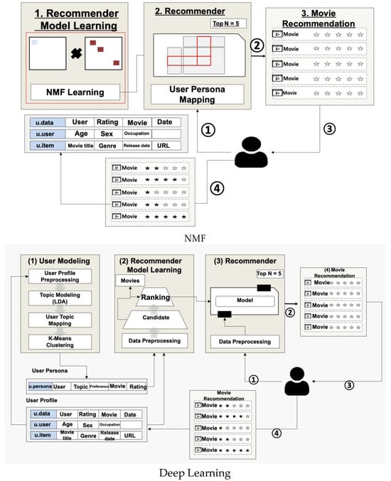
Figure 5.
Movie Recommender System—NMF and Deep Learning Recommendation System using three modules.
The ‘User Modeling’ module uses user information and movie rating data to form user Personas. The ‘Recommender Model Learning’ module trains either the NMF or Deep Learning model based on the created user Personas. Finally, the ‘Movie Recommendation’ module is responsible for recommending specific movies according to user or system requests.
The difference between the two recommender systems lies in the learning method in the ‘Recommender Model Learning’. In the Deep Learning model, the ‘Candidate’ model first extracts candidate movie data, and then the ‘Ranking’ model selects a final movie to be recommended from these candidates.
Figure 6 shows the data flow for generating a user Persona from movie rating data. First, the rating data is collected to form a user corpus. Subsequently, specific topics are assigned to the user through topic modeling, and finally, K-means clustering is used to cluster the users, completing the user Persona.
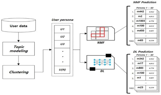
Figure 6.
Composition of Recommendation Algorithm—
User persona generation from movie evaluation data.
We consider the set of movies watched by a user as a document and carries out topic modeling based on this. Figure 7 shows an example of construction by topic modeling user-specific movie data. Each movie belongs to a specific topic, for example, ‘Movie 1’ and ‘Movie 203’ are primarily included in the first topic.
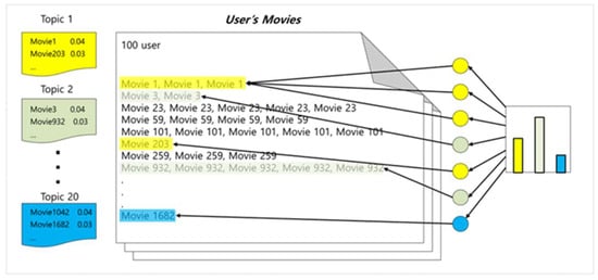
Figure 7.
Topic Modeling of Movie Data.
User’s Movies consists of movies rated by the user, each accompanied by a rating. The topic modeling results for the 100th user show that this user composes Topic1, Topic2, …, Topic20. In this way, topic modeling was performed using movie rating data for a total of 943 users.
We used topic modeling (LDA) and clustering (K-means clustering) techniques to construct user Personas using user data, specifically rating information. These constructed user Personas are trained through the NMF model and Deep Learning model, leading to the construction of a recommendation model. Each model plays the role of predicting the ratings that the user Persona will assign to a specific movie.
The input of the model is the user Persona, and the output is the predicted rating that the user will assign to a specific movie. Based on these predicted values, the Recommender excludes movies that the user has already watched from the remaining movies and makes recommendations to the user.
2.3. Implementation
2.3.1. Dataset
This study used the MovieLens dataset, a real dataset of movie ratings developed by the GroupLens project at the University of Minnesota. The data has u.data, u.item, u.occupation, u.user, and u.genre, with u.occupation and u.genre containing categorical data information [Table 2].
Table 2.
MovieLens Data—movie ratings developed by the GroupLens project at the University of Minnesota.
2.3.2. User Modeling
We present a model that uses user information, movie information, and rating information to model users and generate user Personas. In the preprocessing stage, u.data (user rating information) is used to (1) load and sort the rating data. The data downloaded is loaded using the pandas read_csv library, specifically u.data (data containing user and movie rating information). The data used for data processing is treated as user ID (user_id), movie ID (movie_id), rating information (rating) (u.data contains information about how much rating a user has given to a movie). Afterward, the data is sorted based on the user ID and converted into a numpy array for easy mathematical operations. This is the initial stage of the study, building the basic data needed for creating user Personas and modeling. Such preprocess are essential in machine learning-based recommender systems, as using clean and consistent data can construct more accurate and effective recommendation models. [Figure 8] illustrates the process of preprocessing user data.
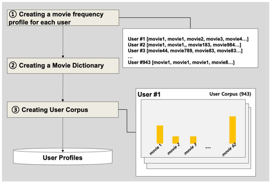
Figure 8.
User data preprocessing.
- (1)
- Creation of movie frequency profile per user
The u.data stores “user, movie, rating, time” data. Step 1 involves assigning weights to the movies that the user has rated highly. In LDA used for topic modeling, the weight in the topic increases if the frequency is high. In this study, the weights are given in the form of “movie ID * rating”, and a variable vector is created by adding the movie ID per user. For instance, if a user named A watches 3 movies and gives 3 points to Movie A, 4 points to Movie B, and 2 points to Movie C, then A user’s movie frequency profile will be [“Movie A”, “Movie A”, “Movie A”, “Movie B”, “Movie B”, “Movie B”, “Movie B”, “Movie C”, “Movie C”]. If A user then watches 2 more movies and gives 2 points and 5 points respectively, A user’s movie frequency profile will be updated to include “Movie D”, “Movie D”, “Movie E”, “Movie E”, “Movie E”, “Movie E”, “Movie E,” resulting in the profile [“Movie A”, “Movie A”, “Movie A”, “Movie B”, “Movie B”, “Movie B”, “Movie B”, “Movie C”, “Movie C”, “Movie D”, “Movie D”, “Movie E”, “Movie E”, “Movie E”, “Movie E”, “Movie E”]. In the LDA model, Movie E would statistically receive more benefit, thus getting a higher weight.

- (2)
- Creation of Movie Dictionary
The movie dictionary consists of movie IDs that hold the implied meaning of the movie. A movie data dictionary, including unique identifier, movie title, release year, genre, etc., is created from the 1682 movies excluding those that did not receive a rating. The gensim’s corpora module was used to create the movie data dictionary. If the movie frequency profile per user is put as an argument, the corpora module creates a word dictionary. The completed word dictionary is stored in the form of Python’s Dictionary, like “{0: 111, 1: 668, 2: 908 …}” in order of index number: occurrence frequency.

- (3)
- Creating a Corpus per User
This step is the process of creating a corpus per user using the movie dictionary and movie information per user, generating 943 corpus data corresponding to the number of users. The completed movie dictionary data and corpus per user are stored in the database. The concept of hashing and mapping can be used to convert words into numbers and check the frequency of those words. It is possible to hash words and map numeric IDs to each word using the doc2bow function with the converted dictionary. This makes it possible to express the words in a document in numbers and check the frequency of those words.

Figure 8 illustrates the process of transformation from Raw data to User Profiles.
The created movie dictionary data and corpus data per user are used to perform topic modeling through LDA. The Coherence Value [12] is calculated to determine the optimal number of topics. We used gensim library to calculate the Coherence Value. As a result, the coherence value results in [Figure 9] can be obtained, and the highest Coherence Value is considered as the optimal number. The coherence value measures how semantically consistent a given topic is. A high coherence value means that the words within each topic are well connected and that the topic expresses a clear subject. Therefore, the highest number was selected to determine the number of topics (60) for the final topic modeling in this study. The result of LDA topic modeling is shown in [Figure 10]. The circles on the left side of the area represent the topics, and the right side represents the words (movies) contained in the topic. In the bar graph on the right, the sky blue represents the total number of words (movies), and the red bar represents the number of movies in that topic. In the end, the movie with the longest red bar is selected as the main movie of the selected topic and becomes the first priority for recommendations.
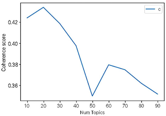
Figure 9.
Coherence Score—determine the number of topics (60) for the final topic modeling.
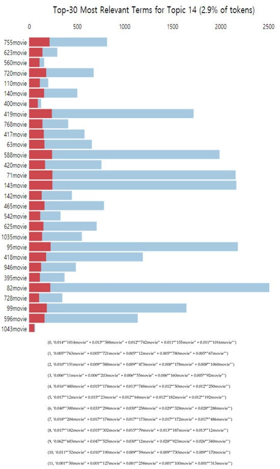
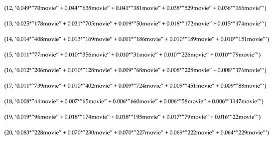
Figure 10.
Topic Modeling Results—the circles on the top side represent the topics, while the down side shows the words (movies) associated with each topic. In the bar chart on the right, the sky-blue bars represent the total number of words (movies), and the red bars represent the number of movies in the respective topic. Ultimately, the movie corresponding to the longest red bar can be one of the main movies of the chosen topic and becomes the top recommendation.
Coherence Values Pseudocode

The ldamodel performs the learning by putting in the corpus, the number of topics (60), and the dictionary as arguments.

The pyLDAvis library visualizes the results. The visualization results of LDA topic modeling are shown in [Figure 10].
A topic is assigned from the completed topics to each user by reading one piece of corpus information at a time. At this point, a user can be assigned multiple topics, which can be considered as the smallest units constituting a user persona. Finally, the user persona is completed by linking it with user topics through performing K-means clustering with the topics of each user.
K-means clustering is an unsupervised learning method. It’s an algorithm that classifies data into ‘K’ clusters and is useful for finding inherent structures or patterns in the data. It is used in various applications, such as customer segmentation, image segmentation, and anomaly detection.
The principle of K-means clustering is to decide the number of clusters ‘K’. This ‘K’ value must be predetermined and choosing an appropriate ‘K’ value has a significant impact on the performance of the algorithm. Secondly, ‘K’ points are randomly selected from the data points to set the initial cluster centroid. For each data point, the distance between the point and each cluster centroid is calculated, and the data point is assigned to the nearest cluster. Once all data points have been assigned to clusters, the center of each cluster is recalculated. In other words, the cluster center is moved to the average location of all data points belonging to the cluster. This process is repeated until the position of the cluster center no longer changes (i.e., until convergence). Due to its relatively low computational complexity and its easy-to-understand nature, K-means clustering is a widely used clustering algorithm. This study used the elbow method to find the optimal K. The elbow method is a way to check the variability of the cluster by gradually increasing the number of clusters. If the variability changes significantly, it means that similar items are well clustered. As shown in [Figure 11], the sum of the distances between the clusters, represented by inertia, dropped sharply at the point where the K value was repeated from 10 to 100, and this value was used as the final number of clusters. [Figure 12] shows the process of completing the user persona.
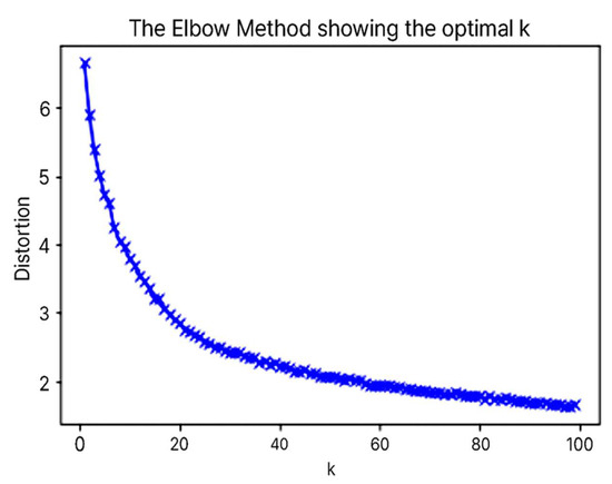
Figure 11.
Optimal K choice from K-mean Clustering.
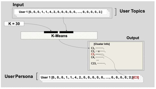
Figure 12.
User Persona Construction.
2.3.3. Recommender Model Learning
We implemented recommendation models using NMF and Deep Learning. The Deep Learning model was implemented by referencing the Deep Neural Network for Youtube Recommendations [Figure 13], and consists of a candidate generation model and a ranking model. The candidate generation model extracts N candidates from large amounts of data, while the ranking model recommends based on the N recommendation target data extracted from the candidates. The NMF model uses movie IDs, user personas, and rating information to train the model and create a Recommender model.
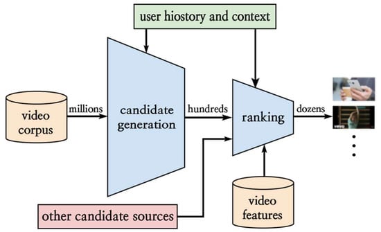
Figure 13.
Deep Neural Networks for YouTube Recommendation—Recommendation system architecture demonstrating the “funnel” where candidate videos are retrieved and ranked before presenting only a few to the user.
The Deep Learning model generates training data with user profiles, user personas, and the movie information viewed by each user. In addition to this information, age data for each movie is created, adding weight to newer movies. The training data created in the data preprocessing process is then used to train the candidate generation model using the artificial neural network model. The movie data extracted from the candidate extraction model is used to add user personal information and train the ranking model. This is done to narrow down the range of large amounts of data that need to be analyzed using the candidate model with limited information and then recommend more accurately using the ranking model. In this study, the candidate model was not used and the ranking model was modified and used as shown in [Figure 14]. [Figure 14] visualizes the process of receiving a user or system request, recommending a movie to the user using the trained NMF model, and providing feedback.
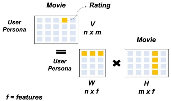
Figure 14.
User Persona Movie Matrix—visualizes the process of receiving a user or system request, recommending a movie to the user using the trained NMF model, and providing feedback.
The first stage is the data collection stage, which includes the process of continuously collecting data by uploading a video and entering meta-information about the video.
The second stage is the candidate extraction stage. In this stage, ‘subnet’ videos suitable for the user are extracted from the video by receiving inputs such as YouTube user’s viewing information, ‘like’, and other feedback, and the candidates are formed. The candidates derived at this point are data that are generally considered suitable for users.
In the ranking decision stage, the data generated in the candidate extraction stage is evaluated and ranked as ‘video itself’, ‘user-centered’, or ‘diversification’. ‘Video itself’ evaluates based on the attributes of the video itself, irrelevant to the user, ‘user-centered’ evaluates based on the user’s taste and environment, and ‘diversification’ includes the process of providing various contents by limiting the provisioning channel of related contents in order to prevent the generation of biased recommendation data with similar specific contents only with the evaluations conducted earlier.
The last stage is the content provision stage, where the content is provided to the user in order from high to low based on the score determined in the ranking decision stage. This allows for personalized content recommendations that match the preferences of users.
2.3.4. Recommender
- (1)
- NMF
Our recommender system used a user persona instead of a rating. The first stage of data collection involves continuously collecting data by receiving meta information about the videos uploaded by users. In the second stage of candidate extraction, the YouTube user’s history of views and “likes” are used as input, and subnet videos suitable for users are extracted from the video to form candidates. These candidates are generally considered to be suitable for users. The third stage, ranking decision, evaluates and ranks the data created in the candidate extraction stage in three stages: the video itself, the center of the user, and diversification. The video itself stage evaluates based on the properties of the video itself, unrelated to the user. The user-centered stage performs an evaluation based on the preferences and environment of the user. The diversification stage provides a variety of contents by limiting the provision of related contents or channels to prevent the creation of recommended data biased towards similar specific contents based on the evaluations conducted earlier.
Figure 15 shows the process of receiving requests from users or the system, recommending movies to
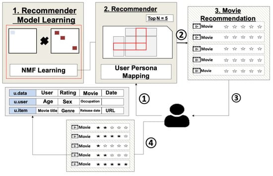
Figure 15.
Recommender—NMF.
- (1)
- A user requests movie recommendation from the Recommender. The Recommender uses the NMF model to generate a user Persona profile based on the movie ratings provided by the user, and maps it to the Persona model.
- (2)
- Excluding movies that the user has already seen, the Recommender recommends to the user movies that are listed in the top N based on hit rate.
- (3)
- The user watches the recommended movie.
- (4)
- The user inputs ratings for the watched movie, and the Recommender generates a profile based on this.

- (2)
- Deep Learning
The trained model creates a candidate pool, and the trained ranking model recommends movies to the user. The candidate model extracts candidate movies for each user and stores them in memory. The stored movie and personal information are added and learned to train the ranking model and complete the model. [Figure 16] shows the process of receiving requests from users or the system and recommending movies to users using the ranking model of YouTube recommendation.
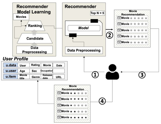
Figure 16.
Recommender—Deep Learning.
We conducted training using a total of 50 epochs, and for optimization, we used adam. Additionally, for the learning rate, we defined a function called step_decay to dynamically change it during training. The function used is as follows.

When the above function is applied, it can be decreased with each epoch and used. Also, we used the default model provided by Keras, including an Input Layer, Embedding Layer, Flatten Layer, Dense Layer, and for layer merging, a Concatenate Layer was used.
- (1)
- The user requests movie recommendations. The Recommender processes the user’s information and recommends the top N movies to the user, excluding movies that the user has already seen, using the results processed through the Deep Learning model.
- (2)
- The user watches the recommended movie.
- (3)
- The user inputs ratings for the watched movie, and the Recommender generates a profile based on this

- (4)
- Model Construction


2.3.5. Movie Recommendation
The user receives movie recommendations from the NMF Recommender and Deep Learning Recommender, watches the movie, and provides evaluation information as feedback. The movie that has received feedback is stored in the User Profiles DB and delivered to User Modeling. Figure 17 represents the data flow until the movie is recommended to the user. First, the user’s ID is delivered to the Recommender, and the Recommender retrieves the user’s information from the Database and delivers it to the trained NMF model. Second, the model retrieves the top N movies based on hit rate. Lastly, the information of the top N movies obtained is delivered to the user. When the NMF model is trained, prediction data (user x movie) is generated, and the top 5 movies are recommended based on the movie information that the user has not rated.
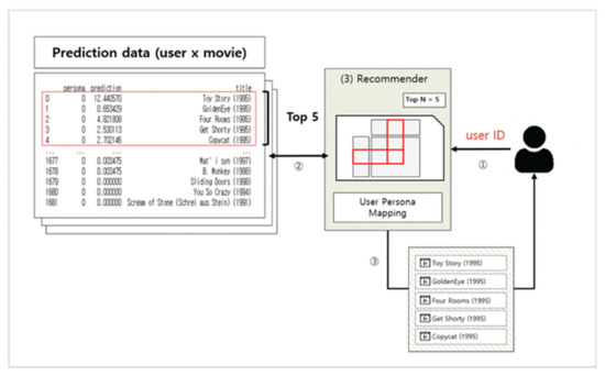
Figure 17.
Movie Recommendation—Data flow of movie recommendation.
2.3.6. Persona Update
The movie evaluation received from feedback is added to the existing user information to assign a user topic, and the user’s Persona information is updated only when the information is changed. [Figure 18] represents the process for updating user Persona. The user Persona update process is as follows: ① The user watches the recommended movie and rates the movie. ② The rating information is added to the user corpus to create another user corpus. ③ A new topic is assigned through the topic model for the new corpus. ④ Which cluster the new topic belongs to is checked. ⑤ Whether the cluster information has changed is checked, and if it has changed, the user Persona is updated to assign a new Persona.
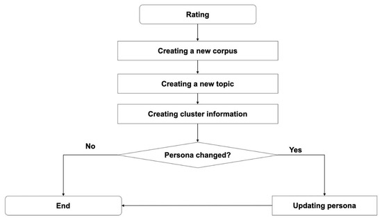
Figure 18.
Persona update Rule.

3. Results
The selection of movie lens data to create a movie recommender system (i.e., data composition) was explained in Section 2.3.1: Dataset. Weights per user was assigned, a corpus was created, and a user-movie Persona was generated based on ratings through LDA (topic modeling) and K-means clustering. A user profile with user corpus and user-movie Persona was created (Section 2.3.2: User Modeling). Each model using NMF and DNN was created with the created profile (Section 2.3.3: Recommender Model Learning), and real movies were recommended (Section 2.3.4: Recommender, Section 2.3.5: Movie Recommendation). Lastly, the Persona Update Rule was defined to automate the model, and the Persona was updated (Section 2.3.6).
3.1. Movie Recommendation Results According to Changes in User Preferences
Subsubsection
We verify that the movie recommendation changes user preferences. We configured the proposed system, selected a random user, and recommended 50 movies over 10 times. The model was selected as the DL model that showed good performance in the top 10, and the selection was conducted according to the Persona update rule. In the case of a movie that belongs to the top 5 genres of movies the user watched, the user gave 2–4 points according to the genre ratio of the recommended movie. Figure 19 is a system configuration to check movie recommendations according to changes in user preferences. The operation method is as follows: ① The user or system requests the recommender system for movie recommendation. ② The requested recommender system checks the user’s information and fetches the user Persona information and puts it as the recommendation model input. At this stage, the model recommends the top 5 movies excluding the movies the user has already watched. ③ The user watches the top N movies and provides the ratings for the movies as feedback to the recommender system. ④ The recommender system stores the user’s movie rating information in the database and sends it to the Persona update module. ⑤ The Persona update module adds the added movie rating information to the existing user corpus, performs the preprocessing procedure, and checks if the Persona has changed after calculating the user Persona. If the Persona has changed, the movie is recommended based on the changed Persona information in step ②. This process is repeated arbitrarily 10 times to accurately update the Persona through repetitive learning.
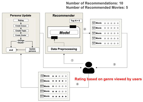
Figure 19.
Movie Recommendation Process according to Changes in User Preferences.
The more movie recommendations are made, the more movies of the genre that match the user’s preferences are recommended, and topic is updated accordingly. Ultimately, the change of the topic means that the individual’s preference is changing, which leads to the change of the user Persona. The initial user Persona is 12 and the topics are Topic 9, 16, and 19 respectively, and the topic contributions are 2, 5, and 3. After watching 35 recommended movies, the user Persona changed from 12 to 22. After the 45th movie was recommended, the Persona changed back to 12. This shows that the user’s latent preferences have changed. The recommended genre confirmed that many representative genre movies were recommended, with Drama increasing from 31 to 55 and Thriller from 19 to 31. [Table 3] presents the recommendation results when the Persona changed due to movie recommendations.
Table 3.
Movie Recommendation Results.
3.2. Evaluation
- (1)
- Evaluation of the Model by Recommended Data
One method for evaluating recommendation models is by computing Precision at K. Precision at K is used when the predicted value is numerical data, with a Threshold value applied to distinguish values equal to or higher than that value as Relevant items and values lower than that value as irrelevant items, to calculate Precision [13]. Here, K represents the top recommended items, or the data with the highest predicted value. The Precision at K method determines relevant and recommended items as shown in [Table 4]. Then, Precision at K is calculated, as shown in [Table 5].
Table 4.
Relevant item and Recommended item.
Table 5.
Precision@K.
Precision at K indicates the proportion of recommended items in the relevant Top-K set. This study set the Threshold value at 3.5 and increased @K from 10 up to 50 in increments of 10 to calculate and evaluate the Precision at K and Hit at K for the NMF and Deep Learning models. The evaluation results showed that the performance of both models decreased as Top K increased. In particular, the rate of performance decrease for the NMF model was higher from Top 30 onwards. Typically, recommender systems focus on finding the top few items related to a user’s preferences. Therefore, the top items in the recommendation list reflect the user’s preferences the best, resulting in the highest values for Precision at K and Hit at K for the top K recommendations.
However, if the value of K is increased, or more items are included in the recommendation list, it is likely that adding items that do not reflect the user’s preferences well increases. This implies that recommended items located in the lower parts of the list are less likely to match the user’s preferences. Therefore, as the value of K increases, or the recommendation list is made longer, the values of Precision at K and Hit at K may tend to decrease.
Especially, the NMF model, being a matrix factorization-based model, might be less effective in capturing complex user behavior or interactions. This implies a relatively faster decrease in performance compared to the Deep Learning model. This feature may account for the faster performance decrease observed in the NMF model from Top 30 onwards. [Table 6] shows the @K metrics of the NMF and DL models.
Table 6.
Precision@k Metrics.
- (2)
- Model Evaluation with MSE
The Mean Squared Error (MSE) metric was used for evaluating topic modeling, Latent Dirichlet Allocation (LDA), Non-negative Matrix Factorization (NMF), and Deep Learning recommender system. MSE is a method of comparing a rating a user actually gives a movie with a rating the same user gives the same movie in the recommender system. For example, if user A gives movie A rating of 4.0 and in the recommender system user A gives a rating of 3.7 to movie A, an error of 0.3 occurs. Therefore, the lower the MSE score, the better the model’s performance. The MSE is calculated as shown in Formula (1), which is the mean of the absolute difference between the actual and predicted values.
Out of 100,000 rating data, 70,000 data were used to train models, and the remaining 30,000 data to evaluate the models. [Table 7] shows the MSE score for each model. For the model without Persona, the DL model showed better performance than the NMF model. The results show that the DL model also outperformed the NMF model with Persona.
Table 7.
Precision@k Metrics—MSEs of NMF and DL were 0.976 and 0.837, respectively without Persona, while with Persona, they were 0.755 and 0.805.
- (3)
- Comparison of Recommendation Time by Model
One user was randomly selected and the time for 1000 movie recommendations was measured. [Table 8] shows the time for each model to recommend 1000 movies.
Table 8.
Time to recommend 1000 movies by model Recommendation times for NMF and DL were 22 ms and 44.9 ms, respectively, without Persona, while with Persona, they were 23 ms and 44.9 ms.
3.3. Data Management According to Persona Application
We examined the difference in the memory or database sizes between with and without applying Persona. Without applying Persona, a matrix of user information of 943 and movie information of 1682 (943 × 1682) is generated. When applying Persona, a matrix of 60 Personas and 1682 movie information (601682) is generated. Although this study used relatively small data and didn’t show significant performance differences, a large matrix in the form of “number of users * number of movies” information is generated if more user and movie information is added. If a fixed Persona is applied, a matrix of “number of Personas * number of movies” information is generated, which can effectively search and learn data. Also, because the number of Personas is fixed, there is no need to update the model by performing learning even if users are added. [Table 9] shows a comparison of matrix sizes between when 60 Personas are applied and when not applied. A matrix of information for 5000 users and 10,000 movies (5000 × 10,000) is generated, and a matrix for 10,000 users and 20,000 movies (10,000 × 20,000) is generated. When applying 60 Personas, the matrix sizes of 5000 users (60 × 10,000) and 10,000 users (60 × 20,000) can be compared.
Table 9.
Matrix Size Before and After applying Persona.
4. Discussion
Through topic modeling using LDA, the recommender system condensed the complex preferences, interests, and favored characteristics of individual users to a lower-dimensional representation; then, the system captured the essence and tendencies of users’ inherent characteristics by completing user personas through k-means clustering based on the results of user topic modeling.
We elucidate the methodologies implemented to mitigate the cold start issue.
Intentional data input through multi-stage recommendations or tournament-style selections, encouraging users to input their preferences. This allows the system to discern user preferences and construct a persona, which is then used to recommend items corresponding to that persona.
Prompting users to create an initial profile at sign-up, which serves as a foundational persona for personalized recommendations.
Generation of provisional user data by assigning popular items or highly rated items as initial data for new users.
Creation of hybrid user data by combining strategies (1) and (3), thus forming a more robust initial user data set.
The essence of the cold start problem lies in the lack of data. To tackle this, we have devised a system where new users are encouraged to fill out initial profiles upon entry, which are then made to be persona. This approach fundamentally resolves the data scarcity issue inherent to the cold start problem, as it allows the system to generate relevant recommendations even for users without historical data.
With user personas, NMF and DL models were implemented to create a movie recommendation service. A comparison of the movie recommendation results was made between NMF and DL models, with and without the use of user personas, using NMF models without personas as the baseline. The results showed that the use of user personas enabled faster recommendations even with an increasing number of users but with a relatively lower precision. A performance improvement in the NMF and DL models with user personas was required. To evaluate the models, we used MSE as a metric, and the NMF model with personas demonstrated lower performance compared to the NMF model without personas in terms of @Precision Top 10, with scores of 94.16% and 92.27%, respectively. As N increased (e.g., Top 50), the performance gap between the two models widened (N-Persona 90.99%, Persona 67.36%). This change is from transforming the relationship between users and ratings to the relationship between personas and ratings. For example, assuming 100 users and that each user has a persona value of 20, the data for 100 users can be compressed to 20. However, obtaining precise recommendations for all users becomes infeasible due to the creation of a matrix with overlapping user and movie information. Regarding the DL model, the one with personas outperformed the model without personas, albeit marginally. With 70 topics and 35 personas, the NMF model achieved a precision@K performance of 65.11% for 100 users, while the DNN (Deep Neural Network) model achieved 80.52% [Figure 20].
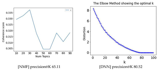
Figure 20.
Precision@K Performance of NMF and DNN with 100 Users under the Conditions of 70 Topics and 35 Personas.
With 200 users, under the same conditions, the NMF model’s precision@K performance improved to 80.01%, and the DNN model’s performance improved to 92.83%, with both showing improvements of approximately 15% and 10%, respectively. [Figure 21].
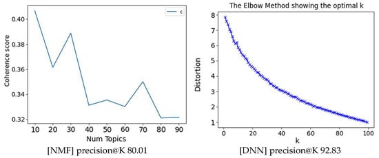
Figure 21.
Precision@K Performance of NMF and DNN with 200 Users under the Conditions of 70 Topics and 35 Personas.
The experiment with 50 topics and 35 identical Personas showed that the NMF’s precision@K performance was measured at 86.01% and DNN’s precision@K performance was measured at 92.67% with 500 user data [Figure 22].
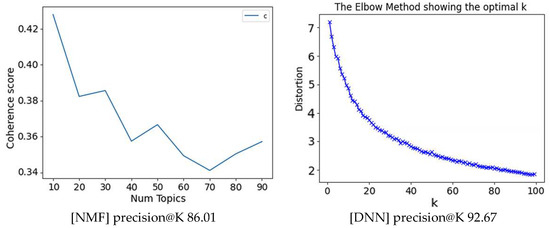
Figure 22.
Precision@K Performance of NMF and DNN with 500 Users under the Conditions of 50 Topics and 45 Personas.
When measured with 50 topics and 45 Persona under the identical conditions and 900 users, NMF’s precision@K performance was 97.04%, and DNN’s precision@K performance was 95.55%, showing performance improvements of 10% and 5% or more, respectively [Figure 23].
Figure 23.
Precision@K Performance of NMF and DNN with 900 Users under the Conditions of 50 Topics and 45 Personas.
These results indicate that the performance improves as the amount of movie rating data and user data increases, allowing it to adapt to changes in user personas. By managing data according to the number of user personas, storage space can be saved, and learning time can be reduced. Additionally, computation costs and time decrease since model updates only occur when user personas change.
The process of creating user personas involves analyzing user behaviors, preferences, habits, and more to form groups with common characteristics. This approach defines groups of users showing similar behavioral patterns or preferences as personas and utilizes them as input for the recommender system. User personas thus created are employed to recommend items that the corresponding user groups are likely to prefer.
Furthermore, merging user personas with other user data enables more sophisticated user modeling. For instance, by jointly modeling user demographic information (age, gender, occupation, etc.), interaction data (movie ratings, click history, etc.), and user behavior patterns that change over time, more personalized recommendations become possible. Integrating user personas with other user data allows for providing recommendations that reflect both individual user characteristics and common characteristics within groups. This surpasses conventional generic recommender systems, enabling highly personalized recommendations and enhancing user satisfaction. It is expected that user personas created in this manner can be utilized in other recommendation services and analyses as well.
Typically, the performance of models improves with the increase in data volume. Our model is no exception to this. For instance, in programs that do not apply topic modeling and personas, the recommendation time is approximately 10 s with an accuracy of 10%. However, when our modeling approach is applied, the recommendation time is significantly reduced to about 3 s, and accuracy is enhanced to 40%.
We believe that these enhancements in our model will allow for more dynamic and adaptable user profiling, effectively addressing the broad spectrum of user interests and their evolution over time.
5. Conclusions
We demonstrated the movies recommendation system based on user personas when a new user is added. However, it is essential to consider the situation when new movies are added. In addition to user personas, creating movie personas presents a novel approach. Movie personas are based on metadata, such as genre, director, cast, and release year. Each movie possesses a unique persona, enabling more sophisticated analysis for movie recommendations. Establishing a model that connects movie personas with user personas makes it possible to identify the movie personas preferred by users and recommend new movies accordingly. For instance, if a specific user persona exhibits a high preference for a particular movie persona, recommending other movies with similar personas becomes feasible. This approach significantly enhances the adaptability to newly added movies. Such an approach finds applications in various domains beyond movie recommendation services. For instance, creating personas for exhibitions or tourist attractions and linking them with user personas is achievable. This enables recommending the most suitable exhibitions or tourist attractions to users by aligning their preferences with the characteristics of the attractions, leading to increased user satisfaction and improved service quality.
When the input format remains the same, our method can be applied to various models. For example, if the previous model used was NMF, it can be replaced with a deep learning model using the same input data. This allows leveraging the strengths of each model and integrating results from different algorithms to achieve more precise predictive capabilities. This approach reminds one of the principles of ensemble learning, which combines multiple models to achieve better performance by allowing each model to approach the given problem from different perspectives. Consequently, using a combination of different models through replacement or ensemble methods can enhance insights and accuracy that were not attainable with a single model alone. This approach proves to be highly useful in improving the performance of recommender systems and can also be applied in the research and development of new recommendation algorithms. In this study, a recommendation algorithm was implemented, generating user personas based on user-rating-movie data to recommend movies to users. Figure 24 illustrates the overall configuration of a user persona and movie persona recommender system. In the future, a movie-centric user recommendation algorithm can be implemented by creating movie personas based on movie-rating-user data. Moreover, we can employ ensemble models such as NMF, DL, Graph Convolutional Network (GCN), among others, to link these two algorithms to constitute the recommendation algorithm.
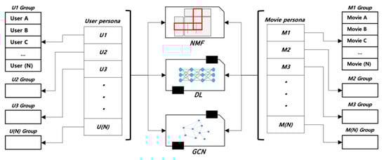
Figure 24.
The overall Configuration of the Persona Recommender System.
The topics of Artificial Neural Networks (AN) and Deep Reinforcement Learning (DRL) are not covered within the scope of this paper. Future research endeavors are planned to extend into the realm of Generative Adversarial Networks (GANs), aimed at processing unstructured data such as images and videos, not just text. Moreover, advancements in accuracy and adaptability will be explored through the application of DRL, which will be a subject of subsequent investigation
Author Contributions
Conceptualization; methodology; formal analysis; data curation; writing—original draft preparation; writing—review and editing, H.-C.L., Y.-S.K. and S.-W.K. All authors have read and agreed to the published version of the manuscript.
Funding
This research received no external funding.
Informed Consent Statement
Not applicable.
Data Availability Statement
The raw data supporting the conclusions of this article will be made available by the authors on request.
Conflicts of Interest
Author Yong-Seong Kim was employed by the company Eum Corporation. The remaining authors declare that the research was conducted in the absence of any commercial or financial relationships that could be construed as a potential conflict of interest.
References
- Koren, Y.; Bell, R.; Volinsky, C. Matrix factorization techniques for recommender systems. Computer 2009, 42, 30–37. [Google Scholar] [CrossRef]
- Lu, J.; Wu, D.; Mao, M.; Wang, W.; Zhang, G. Recommender system application developments: A survey. Decis. Support Syst. 2015, 74, 12–32. [Google Scholar] [CrossRef]
- Chang, Y.; Lim, Y.; Stolterman, E. Personas: From theory to practices. In Proceedings of the 5th Nordic Conference on Human-Computer Interaction: Building Bridges, Lund Sweden, 20–22 October 2008; pp. 439–442. [Google Scholar]
- Available online: https://grouplens.org (accessed on 1 January 2009).
- MacQueen, J. Some methods for classification and analysis of multivariate observations. In Proceedings of the Fifth Berkeley Symposium on Mathematical Statistics and Probability, Los Angeles, CA, USA, 21 June–18 July 1967. [Google Scholar]
- Zhang, S.; Wang, W.; Ford, J.; Makedon, F. Learning from incomplete ratings using non-negative matrix factorization. In Proceedings of the 2006 SIAM International Conference on Data Mining, Bethesda, MD, USA, 20–22 April 2006; Available online: https://epubs.siam.org/doi/10.1137/1.9781611972764.58 (accessed on 28 October 2019).
- Lee, D.D.; Seung, H.S. Learning the parts of objects by non-negative matrix factorization. Nature 1999, 401, 788–791. [Google Scholar] [CrossRef]
- Covington, P.; Adams, J.; Sargin, E. Deep neural networks for youtube recommendations. In Proceedings of the 10th ACM Conference on Recommender Systems, Boston, MA, USA, 15–19 September 2016; pp. 191–198. [Google Scholar]
- Dong, X.; Yu, L.; Wu, Z.; Sun, Y.; Yuan, L.; Zhang, F. A hybrid collaborative filtering model with deep structure for recommender systems. In Proceedings of the AAAI Conference on Artificial Intelligence, San Francisco, CA, USA, 4–9 February 2017. [Google Scholar]
- He, X.; Liao, L.; Zhang, H.; Nie, L.; Hu, X.; Chua, T.S. Neural collaborative filtering. In Proceedings of the 26th International Conference on World Wide Web, Perth, Australia, 3–7 April 2017. [Google Scholar]
- Son, J.; Kim, S.B.; Kim, H.; Cho, S. Review and analysis of recommender systems. J. Korean Inst. Ind. Eng. 2015, 41, 185–208. [Google Scholar] [CrossRef][Green Version]
- Ricci, F.; Rokach, L.; Shapira, B. Introduction to recommender systems handbook. In Recommender Systems Handbook; Springer: Boston, MA, USA, 2010. [Google Scholar]
- Available online: https://github.com/scikit-learn/scikit-learn/blob/main/sklearn/decomposition/_nmf.py/ (accessed on 28 October 2019).
- Blei, D.M.; Ng, A.Y.; Jordan, M.I. Latent dirichlet allocation. J. Mach. Learn. Res. 2003, 3, 993–1022. [Google Scholar]
- Zhang, S.; Yao, L.; Sun, A.; Tay, Y. Deep learning based recommender system: A survey and new perspectives. ACM Comput. Surv. (CSUR) 2019, 52, 1–38. [Google Scholar] [CrossRef]


Disclaimer/Publisher’s Note: The statements, opinions and data contained in all publications are solely those of the individual author(s) and contributor(s) and not of MDPI and/or the editor(s). MDPI and/or the editor(s) disclaim responsibility for any injury to people or property resulting from any ideas, methods, instructions or products referred to in the content. |
© 2024 by the authors. Licensee MDPI, Basel, Switzerland. This article is an open access article distributed under the terms and conditions of the Creative Commons Attribution (CC BY) license (https://creativecommons.org/licenses/by/4.0/).