The Impact of Different Types of El Niño Events on the Ozone Valley of the Tibetan Plateau Based on the WACCM4 Mode

Abstract

This study integrates the sea surface temperature, ozone and meteorological data of ERA5 to count the El Niño events since 1979 and has classified these events into eastern and central types in space as well as spring and summer types in time. The impacts of different types of El Niño events on the ozone valley of the Tibetan Plateau are discussed. The eastern (and spring) type of El Niño events are generally more intense and longer in duration than the central (and summer) type of El Niño events. Overall, in the summer of the following year after El Niño events, the total column ozone (TCO) anomalies near the Tibetan Plateau have a regular zonal distribution. At low latitudes, TCO exhibits negative anomalies, which become more negative approaching the equator. The TCO in the region north of 30° N mainly shows positive anomalies with the high-value region around 40° N. The responses of ozone to different types of El Niño events over the Tibetan Plateau are different, which is further validated by the WACCM4 simulation results. The greater intensity of the eastern (and spring) type of El Niño events caused stronger upward movement of the middle and upper atmosphere in the 20° N region in the subsequent summer as well as a stronger South Asian High. These have resulted in a wider range of negative TCO anomalies in the southern low-latitude region of the South Asian High. In addition, the growing intensity of El Niño extreme events over more than half a century warrants significant concern.

1. Introduction

Stratospheric ozone accounts for approximately 90% of the total ozone in the world and can absorb most of the short-wave ultraviolet rays of the solar rays, thus greatly reducing the intensity of solar ultraviolet radiation reaching the ground. The excessive consumption of stratospheric ozone will lead to the increase in ultraviolet radiation exposure of the biosphere, including human beings, and threaten human life and health [1,2,3,4,5]. In addition, the absorption of ultraviolet radiation by stratospheric ozone will also heat the stratospheric atmosphere, and then affect the temperature field and circulation field of the stratosphere, which is very important to the entire Earth system [6,7].

In 1985, Farman et al. revealed for the first time that the Antarctic stratospheric ozone has been sharply decreasing every spring since the late 1970s, and the trend in ozone reduction continues to strengthen. In 1987, the United Nations invited 26 member states to sign the Montreal Protocol on Substances that Deplete the Ozone Layer, which aims to prevent the continued depletion of the ozone layer [8,9,10].

Since this time, improved observational techniques, especially the launch of satellites, have allowed researchers to more accurately study ozone at all altitudes across the globe [11,12,13,14,15,16,17,18,19]. The researchers found a low ozone value region similar to the Antarctic ozone hole in the upper troposphere–lower troposphere (UTLS) region in the middle and high latitudes of the Northern Hemisphere, known as the “Ozone Valley”. This concept was initially proposed by Zhou and Luo [20], and the valley predominantly spans areas near two major mountain ranges, namely the Tibetan Plateau (TP), known as the third-level roof of the world, and the Rocky Mountains in North America. Between these two ozone valleys, the ozone valley over the TP is the most profound, characterized by the lowest local atmospheric total column ozone (TCO) compared with the areas of the same latitude, especially in summer. Analysis using TOMS (total ozone mapping spectrometer) data has revealed the ozone valley in the TP is formed in summer (June–September), during which time, the discrepancy in the ozone content between the TP and the eastern region at the same latitude could reach 11%.

The significantly low TCO values over the TP have substantially diminished the absorption effect of ozone on solar ultraviolet radiation. Consequently, the ultraviolet radiation reaching the surface is significantly strengthened. In addition, the local snow and rock surfaces, which strongly reflect ultraviolet light, cause Tibet to have a high incidence of cataracts. Therefore, it is very important to study the factors affecting the “ozone valley” of the UTLS layer in the TP region.

Researchers have extensively studied the phenomenon and causes of the ozone valley over the TP [21,22,23,24,25,26,27]. Guo Dong et al. [22] found that the center of the ozone valley is located near the tropopause, with an intensity of approximately −15 DU, and the other sub-strong center is located in the upper stratosphere with an intensity of −8 DU. Zhou Xiuji et al. [28] preliminarily speculated that the dynamic process caused by the special topography of the TP may contribute to the formation of the ozone valley. By studying the characteristics of vertical circulation over the TP, researchers also found that the dynamic and thermal effects of the TP in summer played very important roles in the formation of low-value ozone centers [29,30]. Under the influence of the strong South Asian High (SAH), the updraft of the TP region will form a large amount of divergence in the stratosphere, resulting in a decrease in ozone concentration, while the chemical effect is minimal in this process. At the middle and lower latitudes, the ozone in the middle and lower stratospheres is also affected by the Brewer–Dobson (BD) circulation [31], which is regulated by the El Niño Southern Oscillation (ENSO), prompting researchers to redirect their focus towards investigating the effects of ENSO on the ozone valley [32]. For instance, Chang et al. [33] studied the combined impacts of ENSO and quasi-biennial oscillation (QBO) on ozone in the TP region. They found that the ENSO signal had a six-month advance effect, and the response of the ozone valley was most pronounced in the subsequent summer following the occurrence of an ENSO signal. The ozone valley responds differently to different combinations of ENSO and QBO phases.

ENSO is an important manifestation of the ocean–atmosphere interaction in the tropical Pacific Ocean [34]. ENSO not only affects the circulation of the tropical atmosphere, but the signal can also be transmitted to the middle and high latitudes, and even the polar regions [35,36]. A large number of observations and simulation results show an abnormal accumulation of total ozone during El Niño (EN) in the Northern Hemisphere mid-latitudes and Arctic regions [37,38]. Global warming leads to increased occurrence of extreme EN events, and it is expected that such extreme events will occur more frequently in the future [39,40,41,42,43]. An extremely rare triple-dip La Niña event recently occurred in 2020–2023 [44,45,46,47], and multiple modeling results indicate that the ENSO phase will shift in the second half of 2023, forming a strong EN event (http://cmdp.ncc-cma.net/pred/cn_enso.php, accessed on 1 November 2023), introducing a new round of ozone changes.

Studying the effects of EN on the ozone valley in the TP is critical and necessary. In previous studies, the influence of variable EN events on the ozone valley of the TP is usually analyzed collectively, without meticulous consideration of the diversity in the development time and the spatial pattern of EN. Different types of EN induce various tropical air–sea interactions, and their transmission of signals to the middle and high latitudes differs, greatly affecting the response of the ozone valley on the TP. This study categorizes EN events in time and space, and explores the diverse influences of different types of EN events on the ozone valley over the TP, in combination with the simulation using the Whole Atmosphere Community Climate Model, version 4 (WACCM4).

2. Materials and Methods

2.1. Sea Surface Temperature, Ozone and Meteorological Data

The sea surface temperature (SST), ozone and meteorological data used in this study were derived from ERA5, the fifth-generation reanalysis of global climate and weather from the ECMWF (European Centre for Medium-Range Weather Forecasts) (https://cds.climate.copernicus.eu/cdsapp#!/dataset/reanalysis-era5-pressure-levels-monthly-means?tab=form, accessed on 1 November 2023). These data are used to identify El Niño events and analyze changes in the ozone valley and other atmospheric systems [48]. The horizontal grid resolution of the data is 0.25° by 0.25°, and the vertical height is divided into 37 layers, covering from the ground (1000 hPa) to the stratopause (1 hPa), with a time resolution of months. The period selected in this study includes summer monthly data from 1979 to 2022, and the variables used include SST, the ozone mass mixing ratio, horizontal wind speed, vertical velocity, geopotential, etc.

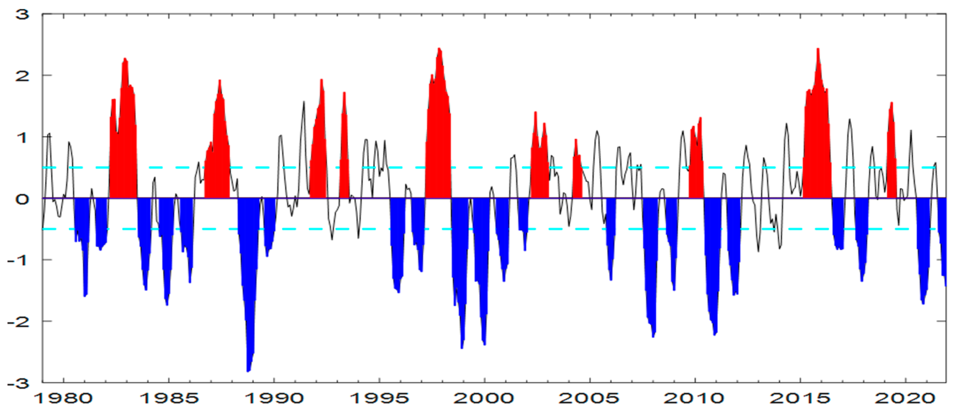
2.2. Classification of EN Events

Using the SST data, the Niño 3.4 index can be obtained by calculating the anomaly of the mean SST relative to the climate mean value (1979–2022) in the Niño 3.4 region (5° S–5° N, 120° W–170° W). An EN event occurs when the three-month moving average of the Niño 3.4 index, consistent with the length of the averaging window used in the Oceanic Niño Index (ONI, https://origin.cpc.ncep.noaa.gov/products/analysis_monitoring/ensostuff/ONI_v5.php, accessed on 1 November 2023), exceeds 0.5 °C for five consecutive months. The statistical time range is from 1979 to 2022 for a total of 44 years. The EN events are classified into eastern (EP) and central (CP) types according to the spatial pattern of SST anomalies of EN events, as well as into spring (SP) and summer (SU) types according to the established time. The specific classification criteria are as follows [48,49,50]:

2.2.1. Classification of EP- and CP-Type EN Events

First, the ${\mathrm{I}}_{\mathrm{E}\mathrm{P}}$ (eastern-type EN index) and ${\mathrm{I}}_{\mathrm{C}\mathrm{P}}$ (central-type EN index) are calculated [50]:

$${\mathrm{I}}_{\mathrm{E}\mathrm{P}}={\mathrm{I}}_{\mathrm{N}\mathrm{i}\mathrm{n}\mathrm{o}3}-\mathsf{\alpha }\times {\mathrm{I}}_{\mathrm{N}\mathrm{i}\mathrm{n}\mathrm{o}4}$$

(1)

$${\mathrm{I}}_{\mathrm{C}\mathrm{P}}={\mathrm{I}}_{\mathrm{N}\mathrm{i}\mathrm{n}\mathrm{o}4}-\mathsf{\alpha }\times {\mathrm{I}}_{\mathrm{N}\mathrm{i}\mathrm{n}\mathrm{o}3}$$

(2)

where ${\mathrm{I}}_{\mathrm{N}\mathrm{i}\mathrm{n}\mathrm{o}3}$ is the Niño 3 index (SSTA of the Niño 3 region (5° S–5° N, 90° W–150° W)) and ${\mathrm{I}}_{\mathrm{N}\mathrm{i}\mathrm{n}\mathrm{o}4}$ is the Niño 4 index (SSTA of the Niño 4 region (5° S–5° N, 150° W–160° E)). To distinguish EP- and CP-type EN events as much as possible, when ${\mathrm{I}}_{\mathrm{N}\mathrm{i}\mathrm{n}\mathrm{o}3}$ $\times$ ${\mathrm{I}}_{\mathrm{N}\mathrm{i}\mathrm{n}\mathrm{o}4}$ > 0, α = 0.4; when ${\mathrm{I}}_{\mathrm{N}\mathrm{i}\mathrm{n}\mathrm{o}3}$ $\times$ ${\mathrm{I}}_{\mathrm{N}\mathrm{i}\mathrm{n}\mathrm{o}4}$ ≤ 0, α = 0. When the absolute value of the ${\mathrm{I}}_{\mathrm{E}\mathrm{P}}$ reaches or exceeds 0.5 °C throughout an event and lasts for at least 3 months, it is considered an eastern-type (EP) event. A central-type (CP) event is defined if the absolute value of the ${\mathrm{I}}_{\mathrm{C}\mathrm{P}}$ during the event is 0.5 °C or more and lasts for at least 3 months. If an event contains both of the above conditions and there is a conversion between the two types, then the type of the event peak is defined as the principal type, which determines the type of the entire event.

2.2.2. Classification of SP- and SU-Type EN Events

Based on the Niño 3.4 index of the three-month moving average, the events with an establishment time (the month in which the first SST anomaly exceeds 0.5 °C) in June and before June are recorded as SP EN, while the events with an establishment time in July and after July are recorded as SU EN [51,52].

2.3. TCO* Calculation for the Ozone Valley

In this study, the ozone mass mixing ratio of 300–50 hPa in the UTLS region is used to calculate TCO [53]:

$${\mathrm{T}\mathrm{C}\mathrm{O}}_{\mathrm{p}1}^{\mathrm{p}2}={\int }_{{\mathrm{p}}_1}^{{\mathrm{p}}_2}0.789\mathrm{M} \mathrm{d}\mathrm{P}$$

(3)

where p is the pressure (units: hPa), M represents the mixed volume ratio of ozone in the atmosphere (units: ppmv), and the resulting TCO is expressed in DU. Then, the zonal deviation of TCO at this point, denoted as TCO*, is obtained by subtracting the average TCO of the entire latitude zone where it is located. The depth of the ozone valley is represented by the value of TCO*.

2.4. Introduction to the WACCM4 Mode

The WACCM4 mode is a three-dimensional global atmospheric mode developed by the National Center for Atmospheric Research [54,55]. This mode adopts the finite volume dynamic framework, with the calculation approach structured as follows: The calculation area is divided into a series of non-repetitive control volumes, with a control volume around each grid point. In this way, the governing equations can be obtained for each grid point and then solved jointly. Therefore, the equation is integrally conserved at any volume. The height of the WACCM4 mode extends from the surface to the lower thermosphere (approximately 145 km), which can effectively reproduce the dynamic, radiation, and chemical processes between the troposphere and stratosphere. It also describes the chemical reaction of the mesosphere and the ion chemistry of the lower thermosphere, etc., meeting the experimental requirements [56]. The horizontal resolution of the mode selected in this study is 1.9° × 2.5°, and the vertical resolution in the tropical tropopause and lower stratosphere is 1.1–1.4 km.

3. Statistics of Different Types of EN Events and Analysis of Their Corresponding Characteristics of the Ozone Valley over the TP

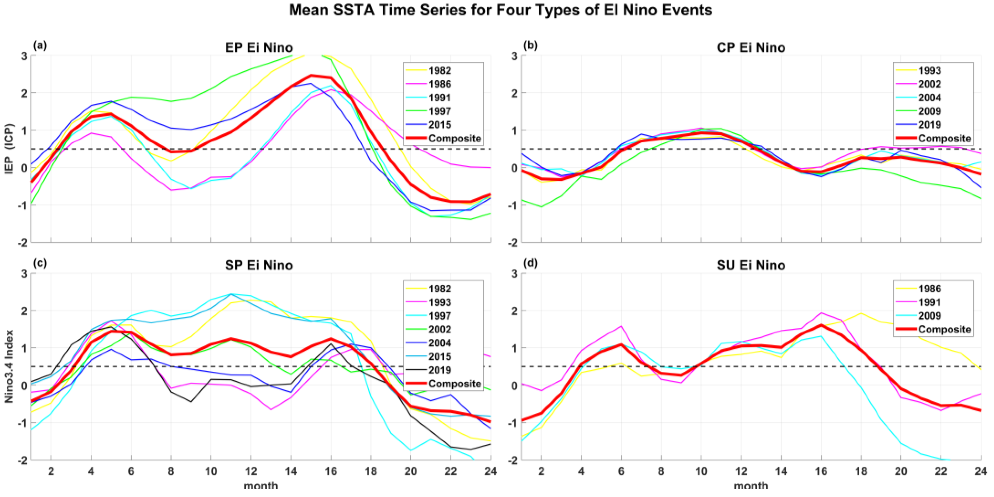
3.1. Classification of EN Events

Using SST data, we recorded the change in the Niño 3.4 index for 44 years from 1979 to 2022, as shown in Figure 1. Then, we classified EN events in time and space accordingly, and the results are shown in

Table 1. Different types of EN events from 1979 to 2022.

Time	Beginning Month	Duration/Month	Spatial Type	Temporal Type	Peak SSTA/°C	Peak Time	Impact Years
1982.03–1983.06	03	16	EP	SP	2.27	1982.12	1983
1986.10–1987.11	10	14	EP	SU	1.92	1987.06	1988
1991.10–1992.06	10	9	EP	SU	1.93	1992.04	1992
1993.03–1993.07	03	5	CP	SP	1.72	1993.05	1993
1997.04–1998.05	04	14	EP	SP	2.44	1997.11	1998
2002.04–2003.01	04	10	CP	SP	1.22	2002.11	2003
2004.04–2004.08	04	5	CP	SP	0.70	2004.07	2005
2009.10–2010.05	10	8	CP	SU	1.31	2010.04	2010
2015.03–2016.06	04	16	EP	SP	2.44	2015.11	2016
2019.03–2019.07	03	5	CP	SP	1.56	2019.05	2019

; they have revealed 10 EN events in the past 44 years. Spatially, there are five EP-type and five CP-type events; while temporally, there are seven SP-type and three SU-type events. In terms of overall strength, the EP (SP)-type is stronger than the CP (SU)-type, accompanied by a longer duration.

The definition of event impact year in Table 1 is based on the results of Chang et al. [33]. Since the response of the ozone valley over the TP to the ENSO signal is strongest in the six months after ENSO, and considering that the peak of the ENSO event is strongest in the winter while the ozone valley phenomenon is most pronounced in the summer, we finally defined the ozone trough time affected by the ENSO peak signal as the most recent summer after the ENSO peak time. This essentially falls in the same year or the following year (later referred to as the following year). For statistical convenience, the classification results of our event impact years are presented separately in

Table 2. Years of summer ozone valley affected by various EN events from 1979 to 2022.

Categories	The Year of the Ozone Valley in the Summer of the Following Year Affected by the Peak of EN Events
EP	1983, 1988, 1992, 1998, 2016
CP	1993, 2003, 2005, 2010, 2019
SP	1983, 1992, 1998, 2003, 2005, 2016, 2019
SU	1988, 1992, 2010

.

3.2. Characteristics of the Ozone Valley over the TP Affected by Different Types of EN Events

The statistical time of the ozone valley over the TP in this study is 44 years from 1979 to 2022. As is shown in Figure 2, the ozone valley is distributed horizontally in the TP and the Iranian Plateau, with a peak central intensity of approximately −1.2 DU.

To demonstrate the influence of EN events on the Tibetan high-pressure ozone valley, the TCO* and TCO results in the summer of the following year of EN are compared with the 44-year mean climate results, and the t-test was carried out to show the intuitive differences (Figure 3). The negative value of the TCO* difference (blue area in Figure 3a) represents a deepening of the ozone valley, i.e., more ozone loss and more UV radiation exposure to the ground. Positive values (red areas in Figure 3a) indicate a shallower ozone valley and an increase in ozone.

It can be seen from Figure 3a that the phenomenon of the ozone valley in the TP region in the following year of EN is weakened. The strongest effect was found in northeast China at 0.21DU. It should be noted that the change in TCO* values here represents the difference in the shape of the ozone valley between the two periods, encompassing the effect of EN on the ozone across the entire latitude circle. Therefore, assessing the specific effects of EN events also requires consideration of TCO variations (Figure 3b), that is, the difference between the total ozone column content without zonal deviation and the climate average. The change in TCO can better measure the influence of EN on the local ozone content.

The overall spatial pattern of TCO presents a relatively regular zonal distribution along the latitude circle. From the equator north to approximately 30° N, i.e., the middle and low latitudes on the south side of the TP, the difference in TCO is negative and becomes more negative approaching the equator. Conversely, north of 30° N, the difference in TCO is mainly positive, with a high-value area near 40° N. The two strong positive anomaly centers emerge in the northeast of China and the northwest of the TP, reaching 0.27 DU and 0.22 DU, respectively. Between 50° N and 60° N, two minor TCO negative anomaly regions are observed, with an intensity of approximately −0.15 DU. The stronger anomaly is located in the western area of Central Russia, northeast of the Caspian Sea, with a central intensity of −0.22 DU.

The regular zonal distribution of the TCO anomaly shown in Figure 3b is related to the changes in BD circulation under the influence of EN. The upward center of the BD circulation in summer moves northward from the equatorial region to approximately 10° N. During EN, SST rises, and the upward motion generated by the tropical ocean–atmosphere convection is strengthened. These intensify the BD circulation, thus promoting the upward motion of the lower atmosphere at the equator and low latitudes. Consequently, more low-concentration ozone at the lower level ascends to the upper level, resulting in a decrease in TCO in the UTLS region. This change corresponds to the negative TCO anomaly of a unified zonal band from north of the equator to near 30° N, as shown in Figure 3b. In the region north of 30° N, due to the strengthening of BD circulation, the atmospheric upward motion will reach a higher height and fall to a more northerly latitude. This will cause a higher-concentration stratospheric ozone in the equatorial region to be transported to the middle and high latitudes and then sink to the UTLS layer, corresponding to the TCO positive anomaly north of 30° N in Figure 3b.

According to the EN categories mentioned above, we separately tabulated the ozone corresponding to the peak values of different types of EN events in the summer of the following year. Subsequently, we conducted the distinct difference test between Figure 3b and the mean climate for each category. In essence, Figure 3b is deconstructed into four modes based on EN types, and the results are depicted in Figure 4.

Various types of EN events exert distinct effects on TCO changes over the TP. As is shown in Figure 3, EP-type EN events (Figure 4a) align with the overall difference in intensity and spatial distribution, with negative anomalies in the southern part of the TP and positive anomalies in the northern part. The range of negative anomalies in the low latitudes extends northward to 30° N, and the weak negative values in the Mediterranean region disappear. The intensity of CP-type EN events (Figure 4b) is generally weak, with a distribution pattern of TCO anomalies distinctive from the overall EN. Influenced by CP-type EN events, TCO in the summer of the following year presents a weak positive anomaly in the region near the Tibetan high pressure, where the high value is still around 40° N of approximately 0.2 DU. The positive anomalies at low latitudes near the equator and the negative anomalies near 60° N are weak and insignificant. Temporarily, the negative anomalies of TCO at low latitudes caused by SP-type EN events (Figure 4c) are weak and not significant. The mid-latitude anomaly is similar to the overall EN. The SU-type (Figure 4d) EN event has the strongest influence, and its TCO positive anomaly center is located near the Caspian Sea, with a value of 0.4 DU. There is a strong negative anomaly from southwest Russia to Eastern Europe, with a value of −0.8 DU.

In conclusion, EN events have significant impacts on the ozone valley over the TP. Moreover, the effects of different types of EN are different in intensity and nature, implying distinct internal influence mechanisms. This prompts further discussion on the influence of diverse types of EN on the ozone valley over the TP.

3.3. Analysis of the Flow Field near the Ozone Valley over the TP Influenced by EN

To understand the mechanism of EN’s influence on the ozone valley in the UTLS layer over the TP, we compared the circulation fields at the 200 hPa layer for different types of EN events with the mean climate state in the summer of the following year, as shown in Figure 5.

Under the influence of different types of EN, the positive (negative) abnormal regions of vorticity at the height layer of 200 hPa (Figure 5a–d) basically correspond to the positive (negative) abnormal regions of TCO at the UTLS layer of 300–50 hPa (Figure 4a, Figure 4b, Figure 4c and Figure 4d, respectively), indicating that the positive (negative) abnormal vorticity at the layer of 200 hPa causes the increase (decrease) in TCO. In general, the positive vorticity of the upper atmosphere corresponds to the upward motion of the lower atmosphere. The strengthening of the upward movement of the lower atmosphere causes an uplift of the low-concentration ozone in the lower layer to the UTLS layer, resulting in a decrease in TCO. In the area south of 30° N, the circulation field at the 200 hPa level in the summer of the following year for each type of EN event is dominated by negative vorticity anomalies. The vorticity-positive anomaly area is mainly distributed near the 40° N zone, corresponding to the TCO-positive anomaly distribution area. Overall, the distribution of each subgraph south of the 50° N zone is roughly the same. Among them, the positive and negative vorticity anomalies corresponding to CP-type EN (Figure 5b) are weak in intensity, and the corresponding TCO anomalies are also weak, which is related to the weak intensity of CP EN events. Comparatively, north of 50° N, there are differences in the distribution of vorticity anomalies. From west to east near 55° N, in the following year after the EP-type EN event (Figure 5a), there is a positive vorticity anomaly on the southwest side of the Caspian Sea with a central intensity of 5.6 × 10⁻⁶/s, a negative anomaly in the north of Kazakhstan and a positive anomaly in the north of Mongolia. After the SP-type EN events (Figure 5c), the negative vorticity anomaly is stronger only in central and southern Russia, which is more easterly than the negative TCO anomaly in the corresponding region (Figure 4c). After the SU-type EN (Figure 5d), a positive vorticity anomaly presents in the northwest of Mongolia and a strong negative vorticity anomaly occurs from south-central Russia to Eastern Europe, with a peak area of 13 × 10⁻⁶/s. This corresponds to the high-value area of the negative TCO anomaly in Figure 4d.

Considering that the SAH is an important weather system in the ozone valley region of the TP, and it has a certain interaction with the ozone [30], we marked the range of SAH in the summer of the following year under the influence of El Niño (black line in Figure 5) and the mean climate of 44 years (yellow line in Figure 5) for comparative analysis. Figure 5 shows that SAH strengthens in the summer of the following year under the influence of El Niño, and the vorticity in the region presents significant negative anomalies. Among them, the distribution areas of the negative vorticity anomalies in the SAH region corresponding to EP-type (Figure 5a) and SP-type (Figure 5c) El Niño events are larger, and the intensity of the high-value region of the anomalies is approximately −6.0 × 10⁻⁶/s. Qin Hao et al. [30] conducted correlation calculations on the three elements of total radiative heating, divergence and vertical velocity of ozone in the UTLS layer and the atmosphere. Their results suggest that when the ozone concentration in the SAH region has a negative anomaly (positive anomaly), the radiative heating is a negative anomaly (positive anomaly) in the lower (upper) ozone valley, causing abnormal convergence (divergence) in the lower (upper) layer. Thus, the ascending lower layer exhibits positive anomalies. The upper-level divergence and the positive anomaly of upward movement finally lead to positive anomalies in the South Asian High. Conversely, the SAH also has an impact on the ozone valley [57]. When the SAH increases, the isotropic surface temperature of 120~50 hPa rises, corresponding to the atmospheric updraft. This additional updraft drives the low-level, low-concentration ozone to rise and reduce the ozone concentration in the region.

Much discussion has been had surrounding how El Niño signals are transmitted to the SAH. Zhang Qiong et al. [58] analyzed the correlation between the SAH and SST in the tropical Pacific Ocean and the Indian Ocean, and the results showed that the SAH has a very close positive correlation with the SST in the Middle East Pacific Ocean and the Indian Ocean, whereas the correlation with the Western Pacific Ocean is very weak. Therefore, we propose the following possible mechanism: El Niño signals first affect the Walker circulation in the vertical direction and cause SST changes in the Indian Ocean through the transmission of the ocean–atmosphere interaction. The rise in the Indian Ocean SST strengthens the SAH through two-stage thermal adaptation and then decreases the ozone concentration near the SAH through the SAH–ozone interaction, especially in the southern region of the TP.

From the above discussion, we find that in the summer of the following year after EN, the low-level updraft corresponds to the negative vorticity anomaly at a low latitude at 200 hPa, and the changes in the SAH will affect the ozone valley over the TP. In the following section, we will further verify this process through the simulation of WMCCM4.

4. Causes of Influence of Different Types of EN on the Ozone Valley Based on WACCM4

The SST fields corresponding to each category of events (Table 1) are monthly averages over 24 months following January at the beginning year, obtaining the SST fields for the four categories with a duration of 24 months (Figure 6). Then, the SSTs for months with an SSTA greater than or equal to 0.5 °C are retained, while the SSTs for other months are synthesized with normal years. This process yields four new SST sequences of 24 months. Subsequently, the SSTs of three normal years are linked to form an EN event with a five-year cycle. Repeating this procedure on a five-year cycle generates multiple EN events to simulate EN signals.

This is an ideal experiment, with the period of 1955–2005, and the SST forcing region applied is 15° S–15° N, 135° E–80° W. The scale of the simulation is global. In four sensitivity experiments (E1, E2, E3 and E4), we introduced the four types of EN SST synthesized above to the forced region to simulate the ozone response to different types of EN events over the TP. To balance the mode, in the first five years (1955−1959), a consistent normal SST was added as the mode start-up phase.

Subsequently, from 1960 to 2005, nine synthetic EN event SSTs were added on a five-year cycle as the SST forcing of the sensitivity test, which was used to replace the SST forcing data specified in WACCM4 for simulation experiments. In this way, we can obtain nine simulated values of the Tibetan high-pressure ozone valley and circulation field in the summer of the following year corresponding to the four types of EN events.

Meanwhile, to facilitate comparative analysis, in the controlled experiment (E0), we input the normal SST for simulation during the whole experimental period. The ozone and flow field data of 51 years from 1960 to 2005 were analyzed. The specific experimental design scheme is given in

Table 3. Design scheme of control experiment and EN sensitivity experiment.

Trial	Added SST Category	Simulation Process
E0	Actual SST	Controlled experiment. Simulation time: 1955–2005. The input SST is normal.
E1	EP EN SST	Sensitive experiment. Simulation time: 1955–2005. The first five years are the start-up years of the experiment, and the normal SST series is added. Then, every five years, the SST forcing of EP EN events synthesized by observations is added in the first two years, and only the SST months with SSTA ≥ 0.5 °C are retained; the other months have a normal SST. The following three years were marked by normal annual SST forcing. The SST forcing range is 15° S–15° N, 135° E–80° W.
E2	CP EN SST	Similar to E1, but with the addition of the composite SST observed by the CP EN events.
E3	SP EN SST	Similar to E1, but with the addition of the composite SST observed by the SP EN events.
E4	SU EN SST	Similar to E1, but with the addition of the composite SST observed by the SU EN events.

. Finally, we compared the nine simulated values of ozone and circulation field over the TP in the summer of the following year corresponding to the four types of EN events. This was simulated by sensitivity experiments with the results of control experiments in the given 51 years (Figure 7 and Figure 8).

The comparison between the simulation results (Figure 7) and the observations (Figure 4) shows great disparities between the TCO and the mean climate results in the summer of the following year of EN. And the simulated values generally align well with the observed results.

From the equator to 30° N, the simulated TCO presents a uniformly negative zonal anomaly of approximately −0.3 DU in the following summer after EP-type (Figure 7a), SP-type (Figure 7c) and SU-type (Figure 7d) EN events. This is consistent with the distribution of observation (Figure 4). There are alternating positive and negative differences between 40° N and 60° N. Under the influence of EP- and SU-type EN events, the TCO is a consistent zonal positive anomaly near 40° N. The signal is strong at approximately 0.8 DU, with the peak area located on the west side of the Caspian Sea and northeast China, and highest at 1.2 DU, consistent with the observed distribution area. There are weak negative anomalies in the TCO near Kazakhstan at 50° N and in the western area of central Russia, and positive ones on the other east and west sides. The TCO under the influence of SP-type EN has a certain negative anomaly in the northwest of the Caspian Sea, which is farther west than the observed location. TCO anomalies in CP-type (Figure 7b) EN events differ significantly from observations (Figure 4b) in the region north of 40° N. In the simulation results, compared with the control experimental results, TCO has a strong zonal negative anomaly of approximately −1.1 DU. Furthermore, the peak area is located northwest of the Caspian Sea and Mongolia region, at −1.6 DU. Compared with the observation data, the negative anomaly of TCO is greatly enhanced and the distribution area is larger. Simulations are improved north of the equator to 40° N, where the TCO anomaly is a weak negative–positive distribution from south to north, consistent with observations.

Figure 8 shows the difference between the 200 hPa flow field simulated by WACCM4 and the controlled experimental climate state in the summer of the following year impacted by different types of EN. Impacted by EP-type (Figure 8a), CP-type (Figure 8b) and SU-type (Figure 8d) EN events north of the equator to 20° N, the flow field presents zonal negative vorticity differences with an intensity of approximately −4 × 10⁻⁶/s, which is in good agreement the observed results. After the SP-type (Figure 8c) EN event, an irregular distribution of positive and negative phases at low latitudes occurs. The simulation has amplified these sporadic weak positive vorticity anomalies in the observations, resulting in a more intense and wider distribution. At 30° N–40° N, the simulation of the four cases is better and shows consistent positive vorticity anomalies of approximately 6 × 10⁻⁶/s; this is in good alignment with the distribution of observed results. At 50° N–60° N, the negative vorticity anomaly is dominant, corresponding to the observed value but with the location slightly shifted. Over the whole region near the ozone valley of the TP, the simulated 200 hPa circulation field anomaly is overall consistent with the observed value, except for substantial positive anomalies of the SP simulation experiment at a low latitude.

To demonstrate the difference in atmospheric movement over the TP under different types of EN events, the wind fields of the four WACCM4 sensitivity experiments were zonally averaged within 20° E–120° E. Thus, the zonal and vertical differences in wind speed between the EP and CP types (Figure 9a) as well as the SP and SU (Figure 9b) types of EN events in the summer of the following year are obtained. In the vicinity of 20° N, EP- and SP-type EN events correspond to a stronger upward movement of the mid-upper atmosphere in the following summer. Meanwhile, the SAH also becomes stronger. These have led to a wider range of negative TCO anomalies, consistent with the observation results (Figure 4) and simulation results (Figure 7).

In summary, the distribution of TCO and flow field at 200 hPa in the summer of the following year of EN simulated by the WACCM4 mode is consistent with the observed results. Furthermore, the positive (negative) vorticity anomalies at this height can correspond to the positive (negative) TCO anomalies. Moreover, the results of the simulation show that in the summer of the following year after EP (SP)-type EN, compared with CP (SU)-type EN, more low-concentration ozone is lifted into the stratosphere due to stronger atmospheric upward movement; the SAH is also stronger during this period, resulting in a larger range of negative TCO anomalies on the south of the TP.

5. Summary and Discussion

5.1. Summary

In this study, the SST data of ERA5 are used to record and classify the EN events in the period of 1979−2022. Combined with the data of the ozone and circulation field, we analyzed the influence of different types of EN events on the ozone valley over the TP. Moreover, the simulation results of the WACCM4 mode further support our conclusions, which are summarized as follows:

(1)

During 1979−2022, there were a total of 10 EN events. From the perspective of event establishment time, there are seven SP-type EN events and three SU-type EN events. According to the spatial pattern of SST anomaly distribution, there were five events of the EP type and CP type, respectively. Overall, the EP (SP)-type events were more intense and lasted longer than the CP (SU)-type events.

(2)

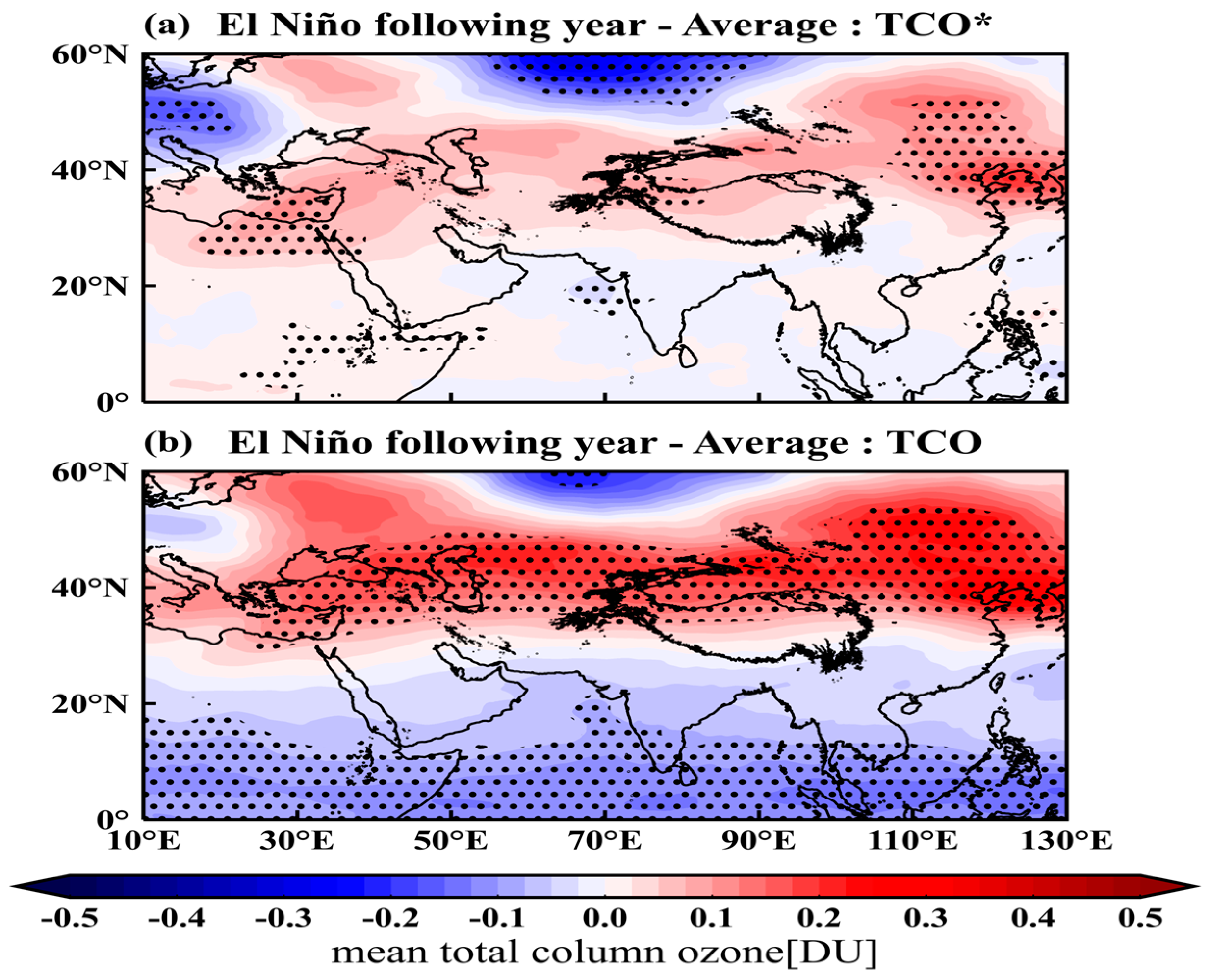
In the summer of the following year after the peak of EN, the ozone valley in the UTLS layer over the TP has a significant change, showing an overall zonal distribution. The calculated differences in TCO show that, on the whole, after EN events, the TCO near the low latitude (0–30° N) presents negative anomalies and becomes stronger nearer to the equator. The TCO variation north of 30° N is mainly a positive anomaly with the high-value area at approximately 40° N, which weakens the ozone valley phenomenon.

(3)

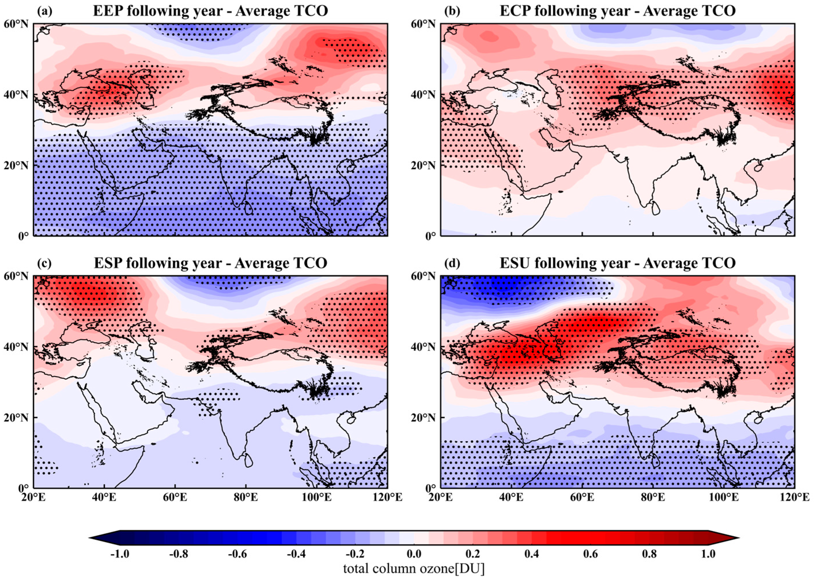
The effects of different types of EN events on ozone in the TP region are distinct in nature and intensity. The EP-type EN is closer to the overall distribution, whereas the distribution of the TCO anomalies of CP-type EN is different from the whole picture. In the range of 10–50° N, the TCO anomaly value is positive, but the overall TCO anomaly value is small. The negative TCO anomaly caused by SP-type EN in low latitudes is weak. The overall effect of SU-type EN is the strongest, with the TCO positive anomaly centered near the Caspian Sea and strong negative effects in the belt from southwest Russia to Eastern Europe.

(4)

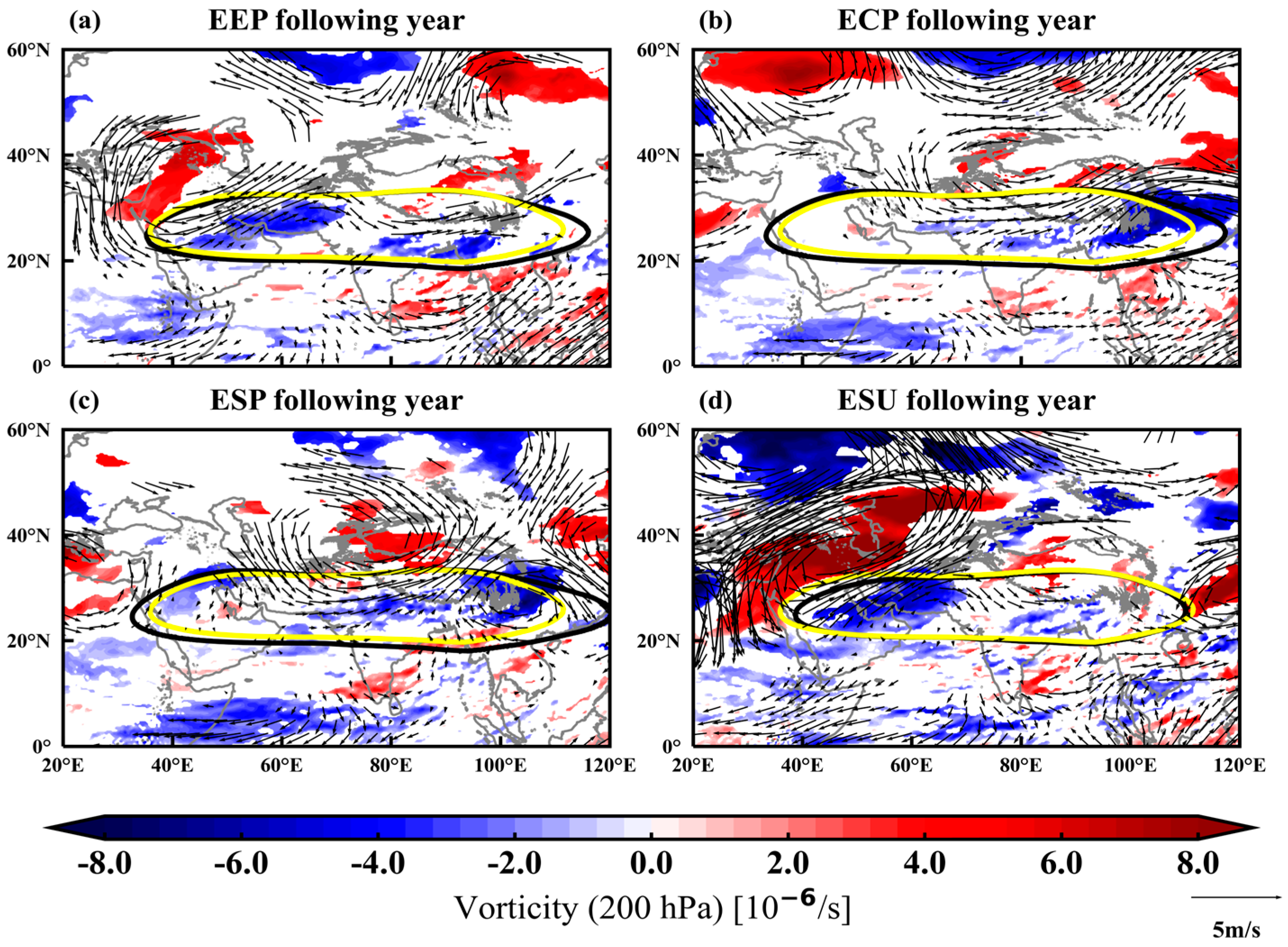
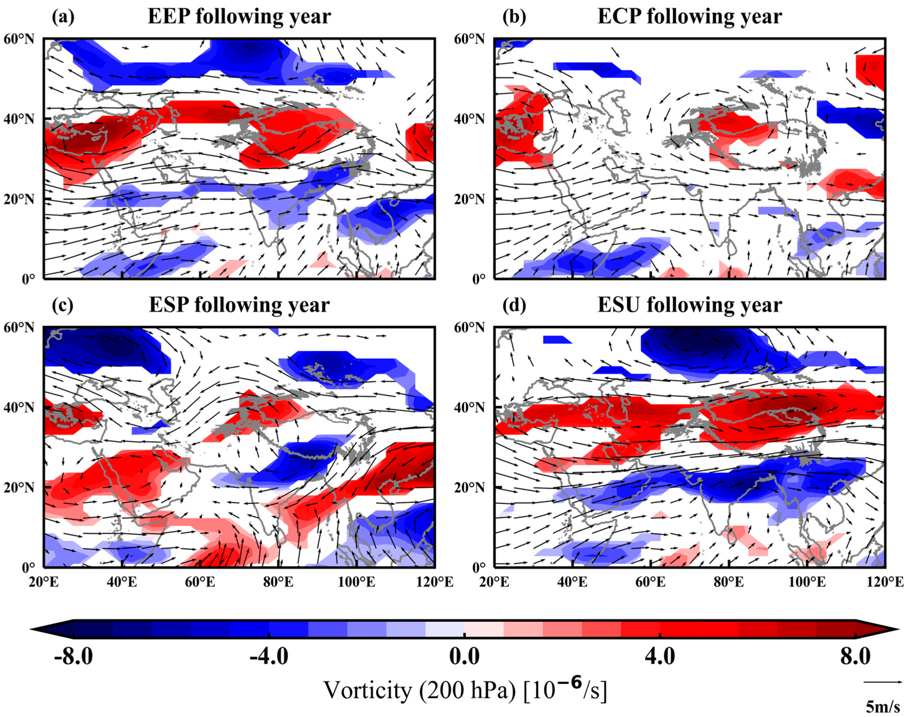
The positive (negative) TCO anomaly in the UTLS layer over the TP in the summer of the following year of EN corresponds to the positive (negative) vorticity anomaly at 200 hPa. In the summer of the following year, at low latitudes, the updraft corresponding to the vorticity anomaly lifts the low-concentration atmosphere of the lower layer to the UTLS layer, resulting in a decrease in the TCO. At the same time, EN causes SST to rise in the Indian Ocean, which enhances the SAH through the two-stage thermal adaptation and then decreases the ozone concentration in the southern low-latitude region of the SAH through the SAH–ozone interaction.

(5)

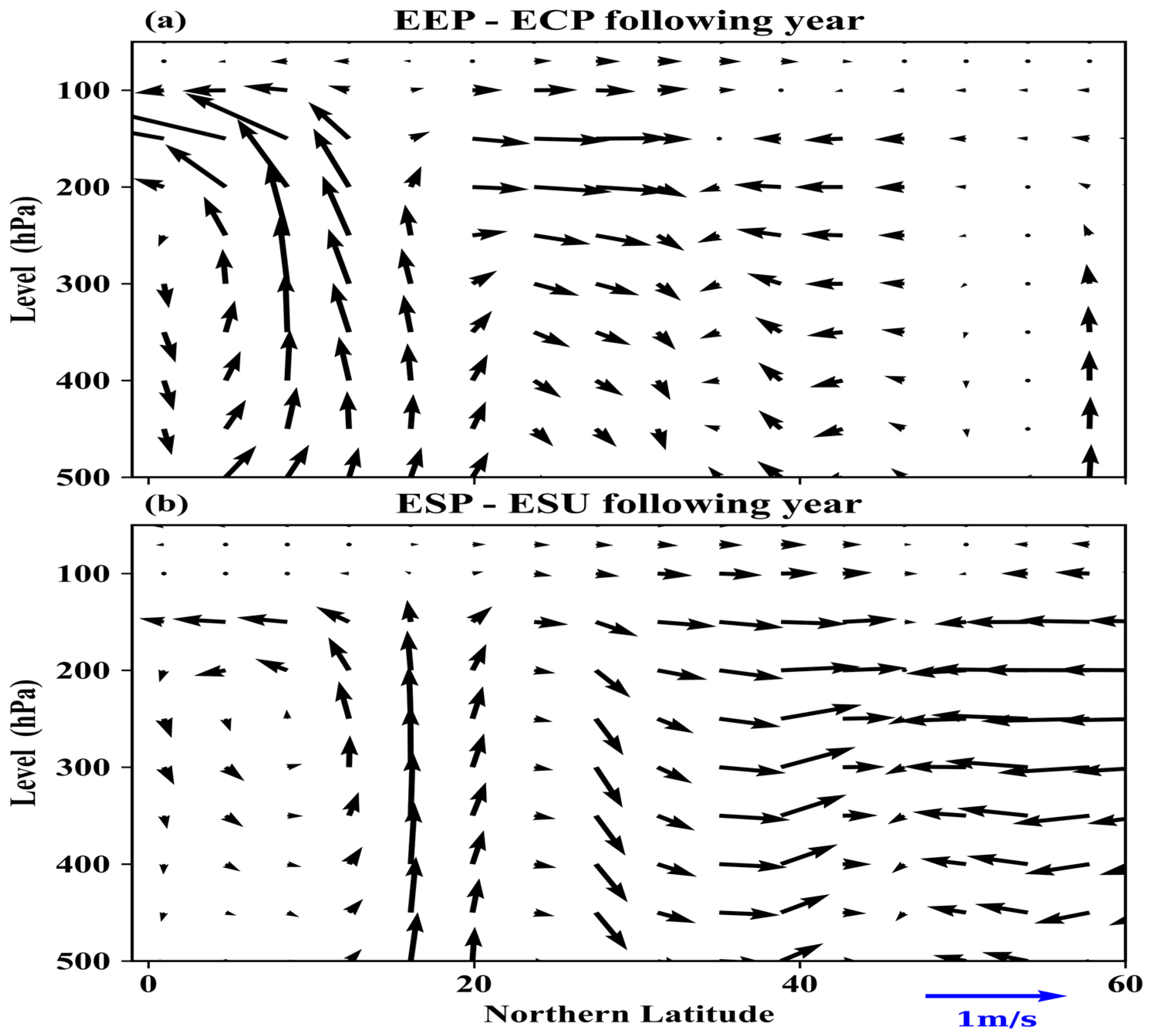
The simulation results of WACCM4 are overall consistent with the observed results, and the vertical profile results further explain the differences between different EN events. Compared with the CP (SU)-type EN events, the middle and upper atmospheric upward movement in the 20° N region near the TP in summer is stronger in EP (SP)-type EN events, and the corresponding SAH is also stronger. Both of these result in a wider range of negative TCO anomalies in the southern low latitude areas.

5.2. Discussion

When recording EN events, although this study only shows the EN events since 1979 calculated using ERA5 SST data, we combined climate data from the NCEP, part of the National Oceanic and Atmospheric Administration, to analyze EN events over a longer time scale since 1950. Statistical results that were not fundamentally different from those of ERA5 were observed. We found that the intensity of EN extreme events (ONI peak SSTA ≥ 1.8 °C) has been gradually increasing over the past half-century. ONI peaked at 1.8 °C in 1958, 2.0 °C in 1965, 2.1 °C in 1972, 2.2 °C in 1982, 2.4 °C in 1997 and 2.6 °C in 2015. Such increases in the intensity of extreme EN events should prompt vigilance and increased awareness. It is also likely to be an example of how extreme weather events have become more extreme since global warming began. Correspondingly, the influence of EN on stratospheric ozone will be greater, highlighting the importance of studying EN.

References

1. Fang, X.; Pyle, J.A.; Chipperfield, M.P.; Daniel, J.S.; Park, S.; Prinn, R.G. Challenges for the recovery of the ozone layer. Nat. Geosci. 2019, 12, 592–596. [Google Scholar] [CrossRef]
2. Chen, Z.; Liu, J.; Cheng, X.; Yang, M.; Shu, L. Stratospheric influences on surface ozone increase during the COVID-19 lockdown over northern China. NPJ Clim. Atmos. Sci. 2023, 6, 76. [Google Scholar] [CrossRef]
3. Diffey, B.L. Sources and measurement of ultraviolet radiation. Methods 2022, 28, 4–13. [Google Scholar] [CrossRef] [PubMed]
4. Antón, M.; Cazorla, A.; Mateos, D.; Costa, M.J.; Olmo, F.J.; Alados-Arboledas, L. Sensitivity of UV erythemal radiation to total ozone changes under different sky conditions: Results for Granada, Spain. Photochem. Photobiol. 2016, 92, 215–219. [Google Scholar] [CrossRef]
5. Zhao, X.; Fioletov, V.; Redondas, A.; Gröbner, J.; Egli, L.; Zeilinger, F.; López, S.J.; Arroyo, A.B.; Kerr, J.; Maillard, B.E.; et al. The site-specific primary calibration conditions for the Brewer spectrophotometer. Atmos. Meas. Tech. 2023, 16, 2273–2295. [Google Scholar] [CrossRef]
6. Tian, W.; Huang, J.; Zhang, J.; Xie, F.; Wang, W.; Peng, Y. Role of Stratospheric Processes in Climate Change: Advances and Challenges. Adv. Atmos. Sci. 2023, 40, 1379–1400. [Google Scholar] [CrossRef]
7. Chipperfield, M.; Bekki, S.; Dhomse, S.; Harris, N.; Hassler, B.; Hossaini, R.; Steinbrecht, W.; Thieblemont, R.; Weber, M. Detecting recovery of the stratospheric ozone layer. Nature 2017, 549, 211–218. [Google Scholar] [CrossRef]
8. Chipperfield, M.P.; Dhomse, S.S.; Feng, W.; McKenzie, R.L.; Velders, G.J.M.; Pyle, J.A. Quantifying the ozone and ultraviolet benefits already achieved by the Montreal Protocol. Nat. Commun. 2015, 6, 7233. [Google Scholar] [CrossRef]
9. Polvani, L.M.; Previdi, M.; England, M.R.; Chiodo, G.; Smith, K.L. Substantial twentieth-century Arctic warming caused by ozone-depleting substances. Nat. Clim. Chang. 2020, 10, 130–133. [Google Scholar] [CrossRef]
10. Son, S.W. Stratospheric ozone loss by very short-lived substances. Nat. Clim. Chang. 2023, 13, 509–510. [Google Scholar] [CrossRef]
11. Cai, X.; Wang, W.; Lin, D.; Eastes, R.W.; Qian, L.; Zhu, Q.; Correira, J.; McClintock, W.E.; Gan, Q.; Aryal, S.; et al. Investigation of the Southern Hemisphere mid-high latitude thermospheric ∑O/N2 responses to the Space-X storm. J. Geophys. Res. Space Phys. 2023, 128, e2022JA031002. [Google Scholar] [CrossRef]
12. Wang, W.; Hong, J.; Shangguan, M.; Wang, H.; Jiang, W.; Zhao, S. Zonally asymmetric influences of the quasi-biennial oscillation on stratospheric ozone. Atmos. Chem. Phys. 2022, 22, 13695–13711. [Google Scholar] [CrossRef]
13. Xie, M.; Gu, M.; Hu, Y.; Huang, P.; Zhang, C.; Yang, T.; Yang, C. A Study on the Retrieval of Ozone Profiles Using FY-3D/HIRAS Infrared Hyperspectral Data. Remote Sens. 2023, 15, 1009. [Google Scholar] [CrossRef]
14. Wang, H.; Wang, W.; Shangguan, M.; Wang, T.; Hong, J.; Zhao, S.; Zhu, J. The Stratosphere-to-Troposphere Transport Related to Rossby Wave Breaking and Its Impact on Summertime Ground-Level Ozone in Eastern China. Remote Sens. 2023, 15, 2647. [Google Scholar] [CrossRef]
15. Hong, J.; Wang, W.; Bai, Z.; Bian, J.; Tao, M.; Konopka, P.; Ploeger, F.; Müller, R.; Wang, H.; Zhang, J.; et al. The Long-Term Trends and Interannual Variability in Surface Ozone Levels in Beijing from 1995 to 2020. Remote Sens. 2022, 14, 5726. [Google Scholar] [CrossRef]
16. Li, Q.; Luo, Y.; Qian, Y.; Dou, K.; Si, F.; Liu, W. Record Low Arctic Stratospheric Ozone in Spring 2020: Measurements of Ground-Based Differential Optical Absorption Spectroscopy in Ny-Ålesund during 2017–2021. Remote Sens. 2023, 15, 4882. [Google Scholar] [CrossRef]
17. Rozanov, S.; Ignatyev, A.; Zavgorodniy, A. Ground-Based Microwave Measurements of Mesospheric Ozone Variations over Moscow Region during the Solar Eclipses of 20 March 2015 and 25 October 2022. Remote Sens. 2023, 15, 3440. [Google Scholar] [CrossRef]
18. Mateos, D.; Antón, M. Worldwide Evaluation of Ozone Radiative Forcing in the UV-B Range between 1979 and 2014. Remote Sens. 2020, 12, 436. [Google Scholar] [CrossRef]
19. Wang, M.; Fu, Q. Changes in Stratosphere-Troposphere Exchange of Air Mass and Ozone Concentration in CCMI Models From 1960 to 2099. J. Geophys. Res. Atmo. 2023, 128, e2023JD038487. [Google Scholar] [CrossRef]
20. Zhou, X.; Luo, C.; Li, J.; Shi, J. The change of total ozone in China and the low value center of the Tibetan Plateau. Chin. Sci. Bull. 1995, 40, 1396–1398. [Google Scholar]
21. Chang, S.; Sheng, Z.; Zhu, Y.; Shi, W.; Luo, Z. Response of ozone to a gravity wave process in the UTLS region over the Tibetan Plateau. Front. Earth Sci. 2020, 8, 289. [Google Scholar] [CrossRef]
22. Guo, D.; Xu, J.; Su, Y.; Shi, C.; Liu, Y.; Li, W. Comparison of vertical structure and formation mechanism of summer ozone valley over the Tibetan Plateau and North America. Trans Atmos Sci. 2017, 40, 412–417. [Google Scholar]
23. Jiao, B.; Su, Y.; Guo, S.; Guo, D.; Shi, C.; Li, J.; Cang, Z.; Fu, S. Distribution of Ozone Valley and Its Relationship with Solar Radiation over the Qinghai-Tibetan Plateau. Plateau Meteorol. 2017, 36, 1201–1208. [Google Scholar]
24. Li, Y.; Xu, F.; Wan, L.; Chen, P.; Guo, D.; Chang, S.; Yang, C. Effect of ENSO on the ozone valley over the Tibetan Plateau based on the WACCM4 model. Remote Sens. 2023, 15, 525. [Google Scholar] [CrossRef]
25. Shi, P.; Chen, Y.; Zhang, G.; Tang, H.; Chen, Z.; Yu, D.; Yang, J.; Ye, T.; Wang, J.; Liang, S.; et al. Factors contributing to spatial–temporal variations of observed oxygen concentration over the Qinghai-Tibetan Plateau. Sci. Rep. 2021, 11, 17338. [Google Scholar] [CrossRef] [PubMed]
26. Chang, S.; He, H.; Huang, D. The effects of gravity waves on ozone over the Tibetan Plateau. Atmos Res. 2024, 299, 107204. [Google Scholar] [CrossRef]
27. Luo, J.; Liang, W.; Xu, P.; Xue, H.; Zhang, M.; Shang, L.; Tian, H. Seasonal features and a case study of tropopause folds over the Tibetan Plateau. Adv. Meteorol. 2019, 2019, 4375123. [Google Scholar] [CrossRef]
28. Zhou, X.; Li, W.; Chen, L.; Liu, Y. Study of ozone change over Tibetan Plateau. Acta Meteorol. Sin. 2004, 62, 513–527. [Google Scholar]
29. Guo, D.; Wang, P.; Zhou, X.; Liu, Y.; Li, W. Dynamic effects of the South Asian high on the ozone valley over the Tibetan Plateau. Acta Meteorol. Sin. 2012, 26, 216–228. [Google Scholar] [CrossRef]
30. Qin, H.; Guo, D.; Shi, C.; Li, Z.; Zhou, S.; Huang, Y.; Su, Y.; Wang, L. The interaction between variations of South Asia High and ozone in the adjacent regions. Chin. J. Atmos. Sci. 2018, 42, 421–434. [Google Scholar]
31. Butchart, N. The Brewer-Dobson circulation. Rev. Geophys. 2014, 52, 157–184. [Google Scholar] [CrossRef]
32. Xie, F.; Li, J.; Tian, W.; Fu, Q.; Jin, F.F.; Hu, Y.; Zhang, J.; Wang, W.; Sun, C.; Feng, J.; et al. A connection from Arctic stratospheric ozone to El Niño-Southern oscillation. Environ. Res. Lett. 2016, 11, 124026. [Google Scholar] [CrossRef]
33. Chang, S.; Li, Y.; Shi, C.; Guo, D. Combined effects of the ENSO and the QBO on the ozone valley over the Tibetan Plateau. Remote Sens. 2022, 14, 4935. [Google Scholar] [CrossRef]
34. Sandweiss, D.H.; Maasch, K.A. El Niño’s role in changing fauna. Science 2022, 377, 1153–1154. [Google Scholar] [CrossRef] [PubMed]
35. Kemarau, R.A.; Eboy, O.V. Exploring the Impact of El Niño-Southern Oscillation (ENSO) on Temperature Distribution Using Remoting Sensing: A Case Study in Kuching City. Appl. Sci. 2023, 13, 8861. [Google Scholar] [CrossRef]
36. Goswami, B.B.; An, S.I. An assessment of the ENSO-monsoon teleconnection in a warming climate. NPJ Clim. Atmos. Sci. 2023, 6, 82. [Google Scholar] [CrossRef]
37. Cagnazzo, C.; Manzini, E.; Calvo, N.; Douglass, A.; Akiyoshi, H.; Bekki, S.; Chipperfield, M.; Dameris, M.; Deushi, M.; Fischer, A.M.; et al. Northern winter stratospheric temperature and ozone responses to ENSO inferred from an ensemble of Chemistry Climate Models. Atmos. Chem. Phys. 2009, 9, 8935–8948. [Google Scholar] [CrossRef]
38. Zhang, J.; Tian, W.; Wang, Z.; Xie, F.; Wang, F. The Influence of ENSO on Northern Midlatitude Ozone during the Winter to Spring Transition. J. Clim. 2015, 28, 4774–4793. [Google Scholar] [CrossRef]
39. Cai, W.; Ng, B.; Geng, T.; Wu, L.; Santoso, A.; McPhaden, M.J. Butterfly effect and a self-modulating El Niño response to global warming. Nature 2020, 585, 68–73. [Google Scholar] [CrossRef]
40. Cai, W.; Ng, B.; Wang, G.; Santoso, A.; Wu, L.; Yang, K. Increased ENSO sea surface temperature variability under four IPCC emission scenarios. Nat. Clim. Chang. 2022, 12, 228–231. [Google Scholar] [CrossRef]
41. Cai, W.; Santoso, A.; Collins, M.; Dewitte, B.; Karamperidou, C.; Kug, J.S.; Lengaigne, M.; McPhaden, M.J.; Stuecker, M.F.; Taschetto, A.S.; et al. Changing El Niño–Southern Oscillation in a warming climate. Nat. Rev. Earth Environ. 2021, 2, 628–644. [Google Scholar] [CrossRef]
42. Geng, T.; Jia, F.; Cai, W.; Wu, L.; Gan, B.; Jing, Z.; Li, S.; McPhaden, M.J. Increased occurrences of consecutive La Niña events under global warming. Nature 2023, 619, 774–781. [Google Scholar] [CrossRef]
43. Lawman, A.E.; Di Nezio, P.N.; Partin, J.W.; Dee, S.G.; Thirumalai, K.; Quinn, T.M. Unraveling forced responses of extreme El Niño variability over the Holocene. Sci. Adv. 2022, 8, eabm4313. [Google Scholar] [CrossRef]
44. Jiang, S.; Zhu, C.; Hu, Z.Z.; Jiang, N.; Zheng, F. Triple-dip La Niña in 2020–23: Understanding the role of the annual cycle in tropical Pacific SST. Environ. Res. Lett. 2023, 18, 084002. [Google Scholar] [CrossRef]
45. Jones, N. Rare ‘triple’ La Niña climate event looks likely—What does the future hold? Nature 2022, 607, 21. [Google Scholar] [CrossRef]
46. Shi, L.; Ding, R.; Hu, S.; Li, X.; Li, J. Extratropical impacts on the 2020–2023 Triple-Dip La Niña event. Atmos. Res. 2023, 294, 106937. [Google Scholar] [CrossRef]
47. Wang, B.; Sun, W.; Jin, C.; Luo, X.; Yang, Y.M.; Li, T.; Xiang, B.; McSpadden, M.J.; Cane, M.A.; Jin, F.; et al. Understanding the recent increase in multiyear La Niñas. Nat. Clim. Chang. 2023, 13, 1075–7081. [Google Scholar] [CrossRef]
48. Chang, S.; Shao, M.; Shi, C.; Xu, H. Intercomparing the response of tropospheric and stratospheric temperature to two types of El Niño onset. Adv. Meteorol. 2017, 2017, 6414368. [Google Scholar] [CrossRef]
49. Kug, J.S.; Jing, F.F.; An, S.I. Two types of El Niño events: Cold tongue El Niño and warm pool El Niño. J. Clim. 2009, 22, 1499–1515. [Google Scholar] [CrossRef]
50. Ren, H.L.; Jin, F.F. Niño indices for two types of ENSO. Geophys. Res. Lett. 2011, 38, L04704. [Google Scholar] [CrossRef]
51. Xu, J.; Chan, J.C. The role of the Asian–Australian monsoon system in the onset time of El Niño events. J. Clim. 2001, 14, 418–433. [Google Scholar] [CrossRef]
52. Yang, J.; Xu, F.; Tu, S.; Han, L.; Zhang, S.; Zheng, M.; Li, Y.; Zhang, S.; Wan, Y. El Niño onset time affects the intensity of landfalling tropical cyclones in China. Atmosphere 2023, 14, 628. [Google Scholar] [CrossRef]
53. Chang, S.; Shi, C.; Guo, D.; Xu, J. Attribution of the principal components of the summertime ozone valley in the upper troposphere and lower stratosphere. Front. Earth Sci. 2021, 8, 721. [Google Scholar] [CrossRef]
54. Arnone, E.; Smith, A.K.; Enell, C.F.; Kero, A.; Dinelli, B.M. WACCM climate chemistry sensitivity to sprite perturbations. J. Geophys Res. Atmos. 2014, 119, 6958–6970. [Google Scholar] [CrossRef]
55. Shangguan, M.; Wang, W. Analysis of Temperature Semi-Annual Oscillations (SAO) in the Middle Atmosphere. Remote Sens. 2023, 15, 857. [Google Scholar] [CrossRef]
56. Ma, X.; Xie, F.; Chen, X.; Wang, L.; Yang, G. Identifying a Leading Predictor of Arctic Stratospheric Ozone for April Precipitation in Eastern North America. Remote Sens. 2022, 14, 5040. [Google Scholar] [CrossRef]
57. Zhou, R.; Chen, Y. Ozone variations over the Tibetan and Iranian Plateaus and their relationship with the South Asia High. J. Univ. Sci. Technol. China 2005, 35, 809–908. [Google Scholar]
58. Zhang, C.; Qian, Y.; Zhang, X. Interannual and interdecadal variations of the South Asia High. Chin. J. Atmos. Sci. 2000, 24, 67–78. [Google Scholar]
Figure 1. Niño 3.4 index record, 1979−2022. The red represents the warm phase and the blue represents the cold phase. The dashed line in light cyan is the threshold of ±0.5 °C.
Applsci 14 01090 g001
Figure 2. Average ozone valley in the Tibetan Plateau region during 1979−2022. The black lines represent the contours of TCO* = −0.6; unit: DU.
Applsci 14 01090 g002
Figure 3. Anomaly of ozone valley over the TP in the summer of the following year of EN during 1979−2022 ((a), TCO*; (b), TCO). The black dots indicate that the difference passes the 95% confidence test; unit: DU.
Applsci 14 01090 g003
Figure 4. Anomaly of ozone valley over the TP under the influence of different types of EN. The black dots indicate that the difference passes the 95% confidence test; unit: DU.
Applsci 14 01090 g004
Figure 5. Abnormal distribution of wind fields at the 200 hPa altitude of different types of EN ((a), EP; (b), CP; (c), SP; (d), SU) in the summer of the following year through a 95% confidence test; unit: 10−6/s. The black line represents the characteristic line of the SAH in the summer of the following year of EN, and the yellow line represents the characteristic line of the SAH in the average climatic state.
Applsci 14 01090 g005
Figure 6. SST indices corresponding to different types of EN events ((a), EP; (b), CP; (c), SP; (d), SU); unit: °C.
Applsci 14 01090 g006
Figure 7. Difference test between TCO and control experiment results of sensitivity experiments of different types of EN ((a), EP; (b), CP; (c), SP; (d), SU) in WACCM4 mode in the following summer. The dotted areas indicate that the differences pass the 95% confidence test; unit: DU.
Applsci 14 01090 g007
Figure 8. Difference test between 200 hPa flow field and control experiment results of sensitivity experiment of different types of EN ((a), EP; (b), CP; (c), SP; (d), SU) in WACCM4 mode in the summer of the following year. The colored region is the vorticity for which the difference passes the 95% confidence test; unit: 10−6/s.
Applsci 14 01090 g008
Figure 9. Latitudinal profile of differences in summer wind velocity of the following year between sensitivity experiments of different types of EN in WACCM4 mode ((a), EP-CP; (b), SP-SU). The vertical wind speed is the result of magnification 500 times.
Applsci 14 01090 g009