Integration of Deep Reinforcement Learning with Collaborative Filtering for Movie Recommendation Systems

Abstract

In the era of big data, effective recommendation systems are essential for providing users with personalized content and reducing search time on online platforms. Traditional collaborative filtering (CF) methods face challenges like data sparsity and the new-user or cold-start issue, primarily due to their reliance on limited user–item interactions. This paper proposes an innovative movie recommendation system that integrates deep reinforcement learning (DRL) with CF, employing the actor–critic method and the Deep Deterministic Policy Gradient (DDPG) algorithm. This integration enhances the system’s ability to navigate the recommendation space effectively, especially for new users with less interaction data. The system utilizes DRL for making initial recommendations to new users and to generate optimal recommendation as more data becomes available. Additionally, singular value decomposition (SVD) is used for matrix factorization in CF, improving the extraction of detailed embeddings that capture the latent features of users and movies. This approach significantly increases recommendation precision and personalization. Our model’s performance is evaluated using the MovieLens dataset with metrics like Precision, Recall, and F1 Score and demonstrates its effectiveness compared with existing recommendation benchmarks, particularly in addressing sparsity and new-user challenges. Several benchmarks of existing recommendation models are selected for the purpose of model comparison.

1. Introduction

In the age of big data, enormous amounts of data from various sources are generated within milliseconds, inundating the information landscape and leading to overwhelming challenges. Recommendation systems emerged long ago as a solution to alleviate this information overload, offering users curated lists of preferred items and helping businesses to optimize user experiences [1]. While many users may benefit from these recommendation models by effortlessly discovering items of interest, businesses generate revenue by showcasing the products that appeal to their customers. Existing traditional recommendation systems include methods like collaborative filtering (CF), content-based filtering (CBF), and hybrid approaches (CF and CBF combination) [2]. These have been known for a long time as popular recommendation techniques. Although these methods assist many people, researchers continue to seek to enhance their effectiveness and to address real-world challenges. Furthermore, traditional methods, like collaborative filtering, often suffer from existing issues, like ”sparsity” and ”new user” problems, particularly the new-user problem as a cold-start issue. While it is relatively easy to search for online items randomly, identifying the most suitable ones for users remains a complex endeavor.

Simultaneously, deep learning has emerged as a powerful paradigm for navigating the complicacy of data, making it particularly well suited in the era of big data for modern recommendation algorithms. Deep learning, often likened to a “black box”, delves deeply into data through hidden layers and subsequently generates outputs. A variety of domains have harnessed deep-learning models to construct highly developed systems. Ferreira, Silva, Abelha, and Machado [3] employed encoder technology to design a recommendation system. Beyond deep learning, reinforcement learning has garnered significant attention from scholars. This progressive approach incorporates essential elements, such as states, actions, environments, and agents, providing a dynamic framework for solving complex problems [4]. Both deep learning and reinforcement learning have become prominent as influential subfields within the extensive domain of artificial intelligence. The use of deep learning is most useful for problems with high-dimensional-state space [5], while reinforcement learning can solve problems of more complicated tasks with lower prior knowledge because of its ability to learn different levels of abstractions from the data [6].

Despite their differing core principles and applications, these two fields share common factors that have contributed to their widespread adoption and recognition in recent years. Furthermore, these innovative methodologies have played pivotal roles in the realm of recommendation systems.

This study offers significant advancements in movie recommendation systems by effectively combining the strengths of DRL and CF, addressing key challenges such as personalization, scalability, and the cold-start problem, with the aim of creating a more robust recommendation system. The main contribution arising from our research works encompasses the following:

• The use of singular value decomposition (SVD) is utilized for matrix factorization in CF, extracting informative embeddings that capture latent user and movie features, which are essential for improving recommendation accuracy and personalization.
• The work emphasizes the actor–critic method within DRL, a strategy that balances policy-based and value-based methods, potentially enhancing the recommendation process. The incorporation of the Deep Deterministic Policy Gradient (DDPG) into the reinforcement learning framework facilitates the training of the recommendation system through continuous interactions between users and the environment, ensuring a flexible and adaptable approach to Top-N recommendation mechanisms. The system updates its internal state to reflect the most recent user interactions, ensuring an up-to-date set of suggestions. To evaluate the performance of the recommender models, several metrics are chosen to measure the proportion of ranking items to ensure that the items are relevant to the target users. Additionally, various benchmark models have emerged for comparison with the support of MovieLens [7].

The structure of the remainder of this paper is organized as follows: Section 2 presents the related works and the relevant concept of recommendation systems, while Section 3 provides the detailed architecture of the proposed works and the implementation flow. Section 4 describes the evaluation metrics used and the selection of benchmarks for comparison purposes and includes the experimental setting and the interpretation of the results. Finally, Section 5 and Section 6 provide the description of the ablation experiments and the conclusions, respectively.

2. Related Work

Recommendation systems have emerged as a necessary technology in the era of big data, effectively tackling the issue of information overload by offering personalized content and service recommendations to consumers [8]. Within this particular area, we classify recommendation systems into three key study domains: traditional-based, deep-learning-based, and reinforcement-learning-based recommendation systems. In addition, the study discusses the challenges and limitations that existed in the traditional approach until the advent of the advanced approach.

2.1. Traditional-Based Recommendation Systems

The traditional recommendation systems comprise collaborative filtering, content-based filtering, and hybrid approaches [9]. Collaborative filtering is a widely employed approach that depends mainly on user–item interactions, covering implicit and explicit data [10]. Content-based filtering is a method that generates user profiles by considering the user’s likes and experiences. Hybrid models have been developed to mitigate the limitations inherent in collaborative and content-based filtering approaches. Goldberg, Nichols, Oki, and Terry [11] established the term “collaborative filtering”, which was the first recommendation system. Later, this technique was enlarged to “recommendation systems” to represent two basic facts: the first is that the approach may not be based on implicit participation by users, while the second refers to the fact that the method may suggest interesting items rather than filter them. The idea of collaborative filtering was intensively researched and made a big impact in the recommendation era. With its attractive usage, researchers discussed collaborative filtering from various perspectives. Additionally, with the growing popularity of recommendation algorithms, Netflix took a major step forward in October 2006 by publishing a comprehensive rating dataset. This release marked the start of a competition to encourage people to improve the recommendation model, ultimately increasing user experiences. The competition aimed to reward the individual or team that could create the most efficient and effective recommendation model with the top prize [12] available. This novel strategy accelerated breakthroughs in recommendation algorithms while also promoting a sense of community and collaboration among data scientists and machine-learning enthusiasts attempting to solve the challenging problem of personalized content recommendations.

Since then, the availability of matrix factorization techniques has risen dramatically, revolutionizing the landscape of recommendation systems. Matrix factorization has become a cornerstone in the creation of sophisticated algorithmic recommendations due to its ability to detect hidden relationships and trends within user–item interaction data [13,14]. This breakthrough has improved the accuracy of recommendations and paved the way for more personalized and effective content suggestions [15]. As a result, when consuming a wide range of products and services from movies and music to e-commerce recommendations, users have been provided with a richer, more customized experience.

While several weaknesses in previous recommendation systems have been resolved, in addition to the advantages of these strategies, there are persisting issues, such as cold-start problems. In response to these persistent obstacles, for entertainment purposes, Xinchang, Vilakone, and Park [16] created a movie recommendation system that took advantage of the benefits of social networking to alleviate cold-start issues in collaborative filtering. To address this issue, the authors created a matrix of user relationships using personal information from users, such as age, gender, and employment. In addition, they employed community detection techniques that rely on edge betweenness to cluster group of users. Vilakone, Park, Xinchang, and Hao [17] utilized community detection techniques to strengthen the recommendation model by employing the k-clique approach. By making improvements to the k-clique method, they successfully developed an effective system for movie recommendations.

Moving from collaborative to content-based filtering, one of the advantages of content-based approaches is their ability to address the user cold-start issue. While content-based approaches include non-user data-based recommendation models, they concentrate on analyzing and comprehending the intrinsic properties of items, such as movies or products, to provide suggestions. This strategy is especially useful when dealing with new users who have not yet provided an adequate interaction history, or when dealing with limited user data. Content-based filtering methods are built upon the attributes of items and the preferences of users. These methods create profiles for users and items based on the attributes or features associated with them [18]. Once the profiles are constructed, items are recommended to a user based on the similarity between the user’s profile and the item’s profile. Additionally, content-based recommendation systems excel at providing personalized recommendations based on individual user interests and preferences. Content-based algorithms can customize suggestions to users by analyzing item features, such as genre, keywords, or traits. This results in a more personalized and relevant user experience. This level of personalization has the potential to boost user satisfaction and engagement with the recommendation platform. For example, in a movie recommendation system, if a user expresses an interest in horror movies, the system recognizes this choice, and recommends other horror movies according to factors such as genre, actors, directors, and keywords to characterize the movie’s content. Recommendation is not only used in the movie industry but is also used more broadly in other sectors. For example, Van Meteren and Van Someren [19] demonstrated a music recommendation system that uses content-based filtering to analyze song audio attributes. This method suggests songs with comparable audio characteristics to the user’s favorites. Similarly, Li, Wang, Li, Knox, and Padmanabhan [20] dig into the benefits of content-based recommendation in the domain of news articles, emphasizing the ability of such systems to offer fresh and diverse items to users based on their reading history and preferences.

However, each method of collaborative filtering and content-based filtering has its own potential to solve the existing problem. Collaborative filtering excels in capturing user–user and item–item interactions to deliver serendipitous recommendations, which is more interesting. It is useful for discovery in recommendation systems, because, unlike content-based filtering, it can uncover hidden preferences and patterns based on collective user behavior. Incorporating content-based filtering techniques into a hybrid recommendation model complements collaborative filtering techniques. This hybrid technique makes use of user–item interactions and inherent item properties to improve the accuracy and robustness of recommendations. For example, content-based features are used as first aid in addressing the cold-start issue for new users. By considering interactions with other users and products, collaborative filtering improves recommendations as the user interaction history increases. Combining both techniques provides an excellent opportunity for another possible solution and solves the weaknesses of both candidates, in addition to enhancing the system performance of recommendations.

Hybrid recommendation systems employ a variety of strategies, such as combining different predictions, fusing characteristics, or unifying models. Tian, Zheng, Wang, Zhang, and Wu [21] suggested a hybrid model that effectively overcomes the drawbacks of both methods, including the cold-start problem, by employing content-based filtering to generate initial recommendations and collaborative filtering to improve them. They created a hybrid model that first uses content-based filtering to find a preliminary list of recommendations, and then refine the list using collaborative filtering to prioritize items based on user–item interactions. This method effectively addresses some of the limitations of both approaches. For example, the cold-start problem, which is a challenge for collaborative filtering, can be mitigated using content-based features. Furthermore, Wang, Wang, and Yeung [22] developed a ground-breaking hybrid strategy incorporating deep-learning methods to capture complicated patterns in item content and user–item interactions. In the area of recommendation systems, there has been a great deal of study, progressing from conventional approaches to deep learning. The models improve with each development, but as the data dynamically increases, new problems appear.

2.2. Deep-Learning-Based Recommendation Systems

Deep learning has recently attracted much attention because of the dynamic nature of data and its extraordinary flexibility in capturing complex patterns and relationships within user–item interactions and content data [23]. This method completely satisfies the demands for modern recommendation algorithms in the big-data era. Additionally, deep learning, which is frequently compared to a “black box”, excels in its capacity to quickly learn from incoming data through hidden layers and then provide valuable outputs. Deep learning automates the feature-extraction process, enabling it to find complex patterns and representations from raw data, in contrast to traditional recommendation systems that frequently rely on handcrafted feature engineering.

In the realm of recommendation systems, deep learning has numerous advantages in the field of decision making. It can process enormous volumes of data, making platforms with massive user populations and diverse categories of suitable items. Because of its capacity to model nonlinear interactions, it can capture user preferences and object features that could be difficult for previous methods to understand [24]. Moreover, the model is also adaptable to a variety of data kinds, including text, graphics, and sequences of user behavior, making it useful in a variety of recommendation domains, including e-commerce, content streaming, and more. Deep learning is also very useful for dealing with problems like the cold-start problem, in which new users or objects have little interaction history. Because of its ability to generalize from the data that is already available, it can be useful for suggestions when conventional collaborative filtering approaches may struggle. In essence, deep learning has become an important tool in recommendation systems, resulting in an era of recommendations that are more precise, flexible, and data-driven [25]. Due to its ability to successfully navigate the complexity of modern data landscapes, deep learning is essential to boosting user engagement and experiences. Additionally, the developments in recommendation systems powered by deep learning have opened the door to investigating cutting-edge ideas, like reinforcement-learning-based recommendation systems. Although deep learning is excellent at identifying patterns and preferences in user interactions and content data, reinforcement learning goes one step further by integrating dynamic decision-making processes that modify suggestions over time in response to user input and interactions [26]. The notion of deep-learning-based recommendation systems is expanded upon as the concept of reinforcement learning is introduced.

2.3. Reinforcement-Learning-Based Recommendation Systems

Deep learning has earned its reputation as a powerful model for extracting insights from complex data. However, the exploration of recommendation systems does not stop there; scholars have also been drawn to the realm of reinforcement learning [27]. Reinforcement learning introduces a unique set of components that include states, actions, environments, agents, and rewards, offering a fresh perspective on how recommendations can be optimized. In reinforcement-learning-based recommendation systems, the user’s interactions with the recommendation platform are viewed as a sequential decision-making process [28]. The “state” represents the user’s current context, while “actions” refer to the recommendation made to the user. The “environment” encapsulates the recommendation system, and the “agent” is responsible for making recommendations based on the user’s state and previous interactions. Rewards are assigned to actions to provide feedback on their quality and relevance. This approach allows recommendation systems to adapt recommendations over time, considering user feedback and interactions to continually improve the relevance and engagement of suggested content. Reinforcement learning holds immense potential for addressing challenges such as the exploration of new items, optimizing long-term user satisfaction, and dynamically adapting to changing user preferences [29].

Several existing works have explored the application of reinforcement learning in recommendation systems. For example, Mlika and Karoui [30] introduced a reinforcement-learning-based recommendation algorithm that models movie-user interactions as a Markov Decision Process, enabling the system to learn optimal recommendation policies. Despite the promise of reinforcement learning, these models often face challenges related to exploration–exploitation trade-offs, scalability, and the need for substantial amounts of user data for training.

Additionally, the integration of reinforcement learning with deep learning has opened up exciting avenues in recommendation systems. Deep reinforcement learning combines the representation-learning capabilities of deep neural networks with the decision-making expertise of reinforcement-learning agents [31]. Researchers have applied this approach to domains like content recommendation, where the system learns to select content that maximizes user engagement and satisfaction. Despite the potential benefits, reinforcement-learning-based recommendation systems present challenges related to the complexity of model training, the need for real-time adaptation, and user privacy concerns. As we delve further into this topic, we explore both the opportunities and challenges that arise in this dynamic field.

3. Proposed System

This section introduces the problem scenarios, model architecture and its algorithm for entire recommendation systems. With the advanced actor–critic technique in deep reinforcement learning, a model of DDPG is used to maximize the reward and optimal policy of the system for the target users (active users).

3.1. Problem Scenarios

We assume that most recommendation systems would best adapt to dynamic environments by rapidly changing user preferences and preachingly recommending the items (movies) to users. However, most of the traditional recommendation models cannot capture the dynamic nature of users/items over time; especially when there is a new update to the system, it is a problem to learn and recommend the closest item to the target users. Some recommendation systems are not focused on a long-term reward.

Given a user u and a movie m for recommendation models, traditional recommendation systems primarily rely on past interactions between u and m to make future recommendations. However, these systems often struggle to account for the evolving tastes and preferences of u over time. How can we harness the capabilities of deep reinforcement learning, specifically the DDPG method, to craft a dynamic recommendation system? The goal is to model the problem of a recommendation system where, for any user u, the system not only considers past interactions with movies but also learns and refines its recommendations, ensuring that movies like m are suggested based on the most current and relevant preferences of u. The scenario is based on reinforcement learning. In a simplified way, we design a dynamic recommendation system using deep reinforcement learning to continuously adapt to change user preferences, maximizing positive user interactions with recommended movies. Moreover, the model surpasses the existing problem of traditional recommendation systems. To formulate suggestions with DRL, the recommendation is specifically modeled as a Markov Decision Process (MDP).

3.2. System Architecture

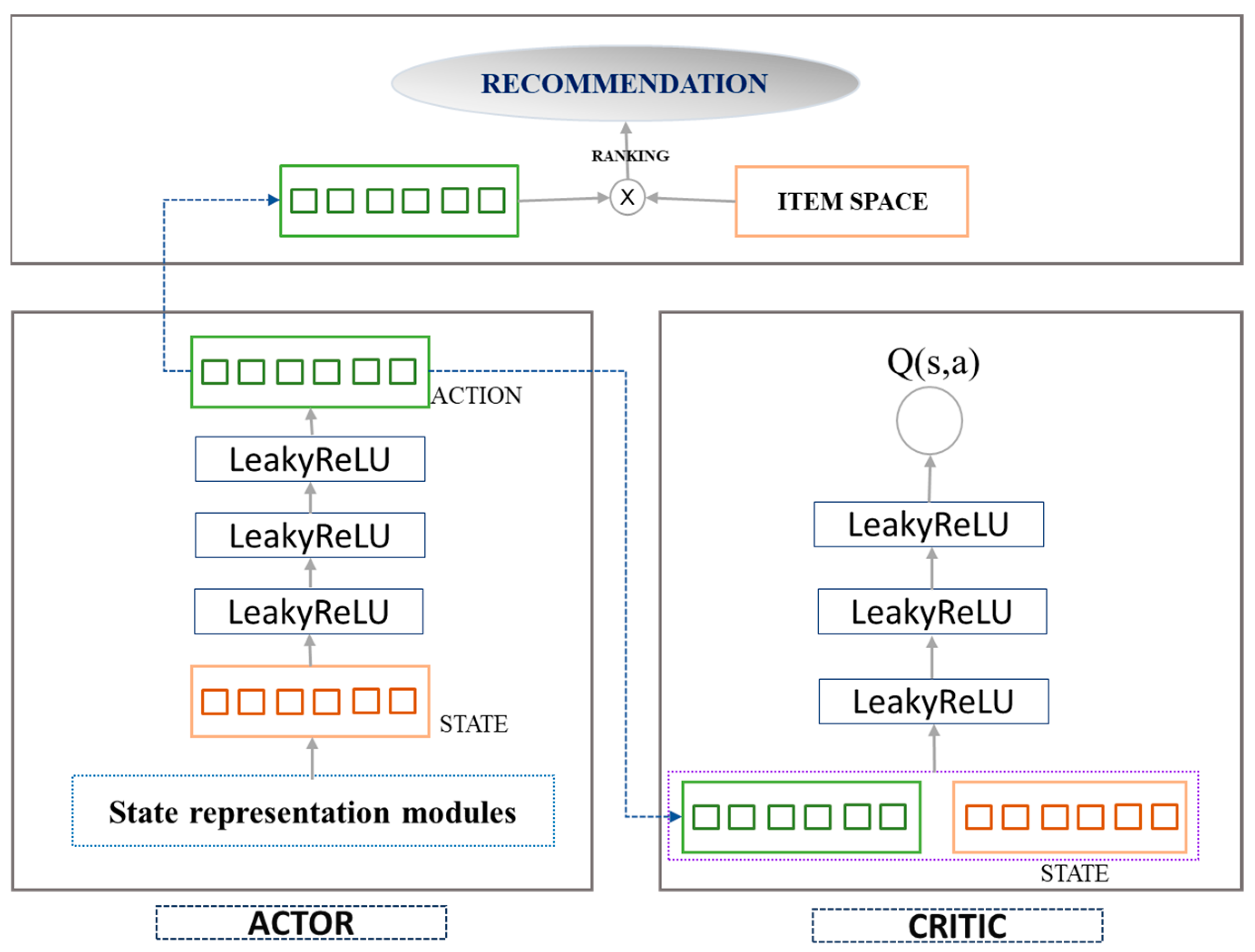
We model the detail of the system architecture in Figure 1. The advantages of this recommendation system model are composed of the following hybrid of policies and values, namely the Actor–Critic Model.

Figure 1. System architecture of the recommendation system.

Figure 1 shows the architecture which describes the recommendation system. As displayed in the above figure, the recommendation system follows the process of the Actor–Critic model. This model is a type of reinforcement learning approach where the actor represents the policy that decides which actions to take, and the critic evaluates how good the chosen actions are. When the model is applied to a recommendation, there is an important module attached to the detail:

State representation modules: The system maintains a representation of the user’s current state, which could include the user’s past interaction, profile data, contextual information, information about the movie, etc. The Actor network takes advantage of the state as input and decides on an action, which, in the context of the recommendation system, would be a list of items to recommend to the target user. In the Critic network, the critic assesses the action taken by the actor by estimating the expected reward (value) of the action, given the current state. This helps in learning which actions (recommendations) are likely to be more successful. In addition, the system uses feedback from the user (such as clicks, watches, ratings) as a reward signal to update both the actor and the critic. The loop allows the system to learn from the user’s behavior and improve over time.

Next, we discuss the advantages of policy learning (actor) and value estimation (critic). In policy learning (actor), the actor directly learns the policy that maps state actions, which can be more efficient than value-based methods, especially in large and complex action spaces that are typical in recommendation systems. Value estimation (critic) helps to reduce the variance of the updates, which can accelerate the learning process and lead to more stable training compared with policy-based methods alone.

Continuous Action Space: Actor–critic methods, especially DDPG, are suitable for problems with a continued action space. With the recommendation system, the continue space could be the user’s interest level in a vast item space. Moreover, with actor–critic models, one can manage the exploration–exploitation trade-off more delicately, which is crucial in recommendation systems to balance between suggesting novel items (movies) and those the user is likely to enjoy. In addition, models can be scaled to handle large user bases and item catalogs, and they can adapt to non-stationary environments (e.g., changing user preferences or evolving the item sets). For experiencing replays in DDPG, this approach can be more sample-efficient, learning effectively from past experiences, and to adapt to real-world issues, the model enables the training process in both online (real-time user interaction) and offline (batch processing) settings, making them versatile for different operational scenarios in the recommendation system.

The involvement of the DDPG will be clearly explained during the implementation process as we intend to provide the detailed flow of the learning procedure in Section 3.3. DDPG can effectively handle continuous action spaces and learn directly from raw, high-dimensional inputs. This makes it an advantageous tool for creating personalized recommendation systems that need to operate in complex and dynamic environments.

3.3. Detail Implementation Flow

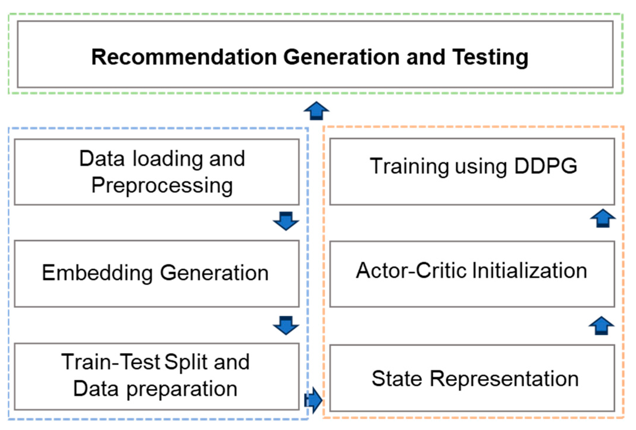
The following diagram illustrates the primary phases within our comprehensive recommender models. To reflect the flow of our proposed recommendation system, we separate the entire system into three phases as shown in Figure 2. The three colors present three different phases which are briefly described in the following subsections. The process begins with the loading of the MovieLens dataset, followed by the implementation of techniques to address the issue of sparse features and their conversion into lower-dimensional features. Subsequently, the data is divided into separate sets for the purpose of evaluation. The next phases involve the development of a DRL model, resulting in the generation of final recommendations as illustrated in the following figure.

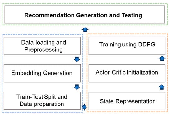
Figure 2. The implementation flow of our proposed system.

3.3.1. Phase One

• Data Loading and Preprocessing

The MovieLens 1M dataset is utilized for performance evaluation. It contains roughly 1 million ratings given by users to movies, with rating scores ranging from 1 to 5. A crucial aspect of this dataset is that it includes user demographics and movie details, which correlate to the rating scale each user applies. Additionally, these ratings encompass approximately 3900 movies and were submitted by 6040 MovieLens users who joined the system in the year 2000. First, User data consist of variables such as userID, movieID, gender, age, occupation, and the user’s zip code. Second, Movie data include movieID, title, and genres. The last one is the Rating file, which is composed of the interaction rating of the userID and the movieID with the specific timestamp variable.

• Embedding Generation

Obtaining embedding provides the ability to learn more detail as the continuous vector representation that captures latent features of users and movies. They represent users and movies in a shared, lower-dimensional latent space, facilitating more efficient and effective recommendations. The generated users and movie embeddings are stored in dictionaries for quick retrieval, especially during the process of recommendation. In our case, singular value decomposition (SVD) is performed on the user–movie matrix to generate the embedding of the movies and users. It refers to the matrix factorization technique commonly used in collaborative filtering. Moreover, it plays an important role in state representation, which will be discussed in the next section.

• Train–Test Split and Data Preparation

We have divided the available user–movie interactions into training and testing sets. This division is important for performance evaluation, especially the recommendation on unseen data (related to tests on user cold starts). Three-quarters (75%) of the dataset is used for training the recommendation model, and the remaining 25% is for evaluating its performance on unseen data. Ensuring that the model is tested on a separate set helps to assess its generalized ability and provides an unbiased estimate of its performance. The dataset is prepared to include the information such as userIDs, movieIDs, ratings, and timestamps. Users with a positive rating count greater than 10 are selected for the training set. Both the training and testing datasets are filtered to ensure that they contain only unique IDs, with no duplication.

3.3.2. Phase Two

• State Representation (AdaptiveMaxPool State Representation)

The study details how the state representation is determined, a crucial aspect in deciding the “state” used by the recommendation system and learning model. This component is essential for the model to understand the user’s preferences and to make a good recommendation. Moreover, state representation plays a significant role in both the Actor and Critic network. This representation generates the current state of the user based on user-feature information and the user’s historical movie-feature interaction matrix. Figure 3 illustrates the state representation module, the user-feature matrix, and the movie features (e.g., Movie 1, Movie 2, Movie 3 and Movie N). The state is formed by concatenating and flattening user features with movie features, followed by an AdaptiveMaxPool operation. The Adaptive Pooling block is a type of pooling operation that resizes the input to a predefined output size. The block of the “concat and flatten” step implies that data from different sources are concatenated into a single vector and then flattened into a 1D tensor. Concatenation happens in the state representation module when user embeddings, movie embeddings, and their element-wise product are concatenated to form a state. Furthermore, this process is very necessary to the Actor and Critic networks as they both take the state as input to generate actions and evaluate them.

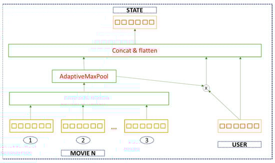
Figure 3. State representation of movies and user features.

• Actor–Critic Initialization

The proposed recommendation applies an Actor and Critic architecture using DDPG for initialization. Actor Network initialization: defining the neural network architecture for the actor, this network architecture takes the state (user’s profile, movie, historical interactions) as input. Next, we initialize the network weights, typically with small random values to break the symmetry. Xavier initialization is used for the initial weight, ensuring that the initial weights are neither too high nor too low. Both the Actor and Critic networks use fully connected (dense) layers. These are standard neural network architectures for processing high-dimensional input data. The Actor network consists of three linear layers (linear1, linear2, linear3). These layers are responsible for processing the state input and outputting the action (recommendation). The Critic network also has three linear layers (linear1, linear2, linear3), but it processes both the state and the action together, outputting a single value that estimates the Q-value of the state–action pair. The first linear layer in both networks serves as the input layer, receiving either the state (Actor) or state–action pair (Critic) and beginning the process of feature transformation. The subsequent layers (often called hidden layers) further process these inputs, allowing for more complex representations and interactions between features. They are crucial for learning the non-linear relationships in the data. The final layer in the Actor network outputs the action, while in the Critic network, it outputs the Q-value estimation. These are keys for decision making (Actor) and evaluation (Critic). The Actor generates movie recommendations, and the Critic evaluates the quality of those recommendations. Moreover, the network architecture will typically include an input layer and one or more hidden layers with dropout and non-linear activations like Relu or Leaky Relu; in our case, we choose Leaky Relu for the activation function. The use of dropout layers and activation functions helps with regularization and introduces non-linearity into the network, as illustrated in Algorithm 1.

Algorithm 1 Actor–Critic Model Initialization
	Define the Actor class Inherits nn.Module:
		Initialize neural network layers:
			Linear(input_dim,hidden_dim)->LeakyReLU->Dropout(optimal_prob)
			Linear(hidden_dim,hidden_dim)->LeakyReLU->Dropout(optimal_prob)
			Linear(hidden_dim, output_dim)
			#Second Linear layer from hidden_dim to hidden_dim
			LeakyReLU activation layer
		Define forward(state):
			state -> Linear1->LeakyReLU ->Dropout ->Linear2->LeakyReLU->Dropout->Linear3
			return output
	End Actor Class
	Define the Critic class Inherit from nn.Module
		Initialize:
			Linear(input_dim+output_dim, hidden_dim)->LeakyReLU->Dropout(optimal_prob)
			Linear(hidden_dim, hidden_dim)->LeakyReLU->Dropout(optimal_prob)
			Linear(hidden_dim, 1)
			Initialize weights of last layer uniformly within specified range
		Define forward(state, action):
			Concatenate(state,action)->Linear1->LeakyReLU->Dropout->Linear2->LeakyReLU->Dropout->Linear3
			return value_estimate
	End Critic Class
	Model Initialization:
		Set input_dim, output_dim, hidden_dim as per dataset characteristics
		actor = Actor(input_dim, hidden_dim, output_dim, dropout_probability)
		critic = Critic(input_dim, output_dim, hidden_dim, dropout_probability)
		actor_target = actor_model
		critic_target = critic_model
	Define Optimizers:
		actor_optimizer = Optimizer(actor.parameters(), learning_rate)
		critic_optimizer = Optimizer(critic.parameters(), learning_rate)

• Training using the DDPG

The Deep Deterministic Policy Gradient (DDPG) is an actor–critic model-free algorithm designed for solving problems with continuous action spaces, making it particularly suitable for reinforcement-learning tasks. Specifically, the algorithm extends concepts from Deep Q learning to handle continuous action spaces by combining elements. The following Algorithm 2 is for training the DDPG and is processed as follows:

Algorithm 2 DDPG Training
	Initialize Networks and Parameters:
		actor_model = initialize_actor_network(input_dim, hidden_dim, output_dim)
		critic_model = initialize_critic_network(input_dim, output_dim, hidden_dim)
		actor_target = actor_model
		critic_target = critic_model
		replay_buffer = create_replay_buffer()
		Set exploration_noise, discount_factor, tau (soft update parameter)
	Training Loop:
		For episode = 1 to max_episodes do:
			initialize exploration_noise
			state = observe_initial_state()
			for t = 1 to max_timesteps do
				action = actor(state) + exploration_noise
				next_state, reward, done = execute_action(action)
				replay_buffer.store(state, action, reward, next_state, done)
				batch = replay_buffer.sample()
				target_Q = compute_target_Q(batch, critic_target, actor_target, discount_factor)
				update_critic(critic, batch, target_Q)
				update_actor(actor_model, critic_model batch)
				soft_update(actor_target, actor_model, tau)
				soft_update(critic_target, critic_model, tau)
				update exploration_noise
				if done then
					break
				end if
			end for
		end for

3.3.3. Phase Three

This phase of the development system involves rigorously testing the recommendation system with a diverse set of users not seen during training and focusing on generating accurate recommendations.

• Testing and Recommendation Generation

In the final phase of the recommendation-system development, we undertake the crucial task of system evaluation and recommendation generation for users. To ensure the robustness of our assessment, we employ a randomization of userIDs to ensure a fair test; i.e., userIDs are chosen randomly for testing. This method helps to avoid bias because the system has not seen these users during their training phase. Addressing cold-start scenarios, a common challenge in recommendation systems is dealing with new users who have very little interaction history (known as “cold start” users). To tackle this, users who have given fewer than 10 high ratings (rated 4 or 5) are intentionally excluded from the test set. Another point is the separation from the training data; by ensuring that the users selected for testing are not from the training dataset, the system’s evaluation becomes more reliable and freer from biases that could arise if it were tested on familiar data.

3.4. Algorithms for the Proposed System

In this section, we show the entire algorithm for our recommendation system. Following the implementation section, we keep the same structure, and the process of overall system starts as shown in Algorithm 3.

Algorithm 3 The Proposed System for Movie Recommendation system
Input: ratings_df, movies_df, users_df
Output: evaluation_metrics, specific user_recommendations, top-N recommendation
Procedure:
	1: Load and preprocess data:
		ratings_df, movies_df, users_df = load_movie_data()
		R_df = create_user_item_matrix(ratings_df)
	2: Split data into training and testing sets:
		train_users, test_users = split_users_based_on_ratings(R_df)
	3: Prepare data for deep reinforcement learning:
		train_dataloader, test_dataloader = create_data_loaders(train_users, test_users)
	4: Initialize reinforcement learning models:
		actor_model = initialize_actor_model()
		critic_model = initialize_critic_model()
		target_actor_model = actor_model
		target_critic_model = critic_model
		replay_buffer = initialize_replay_buffer()
	5: Define state representation:
		define_state_representation_functions()
	6: Train the models—for the detail refer to Step 2:
		for episode = 1 to num_episodes do
				for batch in train_dataloader do
					state = compute_state_representation(batch)
					action = actor_model(state)
					reward = calculate_reward(batch)
					next_state = compute_state_representation(batch)
					replay_buffer.push(state, action, reward, next_state)
					if replay_buffer.size() > batch_size then
						update_actor_critic_models(replay_buffer)
					end if
				end for
		end for
	7: Test the models:
		for batch in test_dataloader do
			state = compute_state_representation(batch)
			recommendations = generate_recommendations(actor_model, state)
			evaluate_recommendations(recommendations, batch)
		end for
	8: Compute evaluation metrics:
		evaluation_metrics = calculate_evaluation_metrics()
	9: Generate user-specific recommendations:
		selected_user_id = choose_user_id(test_users)
		user_recommendations = generate_user_specific_recommendations(selected_user_id)
	10: Analyze recommendations using cosine similarity:
		cosine_similarity_matrix = compute_cosine_similarity(user_recommendations)
	11: Return Output

4. Experiments and Results

In this section, we conduct extensive experiments with a dataset from GroupLens, which includes approximately 1 million movie ratings. Moreover, we introduce essential tasks in our system, including the experiment settings, evaluation metrics, benchmark methods, and the discussion results.

4.1. Experiment Setting

The current study utilizes several tools to support the implementation process, including Python version 3.9, Torch, Pandas, Numpy, and Matlibplot for visualization. Additionally, we have developed the entire model on a Windows OS platform with a RAM capacity of 64 GB. For evaluation, we use the MovieLens 1M dataset, which comprises 1,000,209 anonymous ratings for a total of 3900 movies. These ratings are collected from a user base of 6,040 individuals who joined MovieLens in the year 2000. We select users who have rated movies with a rating greater than 3 and have provided more than 10 ratings. Additionally, we choose an embedding size of 100 for the MovieLens datasets. For the initial parameters, the dropout is set to 0.6, with a hidden size of 128 and 256, both for the Actor and Critic networks. There are several optimizers that are used for model tuning. Adam, Adadelta, Adamax, RMSprop, and SGD are involved for the purpose of finding the optimal recommendation result. The learning rate of each optimizer is set to 0.0001. We use a gamma value (discount factor) equal to 0.98 to determine the importance of future rewards. Some optimizers support with momentum; for these, we set the value to 0.9, since this is the most recommended value.

4.2. Evaluation Metrics

Three common metrics are selected for the purpose of evaluation in recommendation systems. Precision, Recall, and the F1 Score are used for evaluating and fine-tuning recommendation systems and other retrieval algorithms, ensuring that they provide relevant and comprehensive results. Precision@k measures how many of the top-k-recommended items are relevant or true positives. Recall@k is used for measuring the proportion of relevant items that are found in the top-k recommendations. It is important for understanding how many of the total relevant items are captured in the top-k recommendation. Another metric is the harmonic mean of Precision and Recall. It is a way to combine both metrics into a single, overall measurement of the model’s accuracy. This technique is useful when we need to balance Precision and Recall. Precision@k, Recall@k and F1 Score will be abbreviated and formed as below:

$$\mathrm{P}\mathrm{r}\mathrm{e}\mathrm{c}\mathrm{i}\mathrm{s}\mathrm{i}\mathrm{o}\mathrm{n}@\mathrm{k}=\frac{\# \mathrm{o}\mathrm{f} \mathrm{r}\mathrm{e}\mathrm{l}\mathrm{e}\mathrm{v}\mathrm{a}\mathrm{n}\mathrm{t} \mathrm{i}\mathrm{t}\mathrm{e}\mathrm{m}\mathrm{s} \mathrm{a}\mathrm{m}\mathrm{o}\mathrm{n}\mathrm{g} \mathrm{t}\mathrm{h}\mathrm{e} \mathrm{t}\mathrm{o}\mathrm{p}\mathrm{k} \mathrm{r}\mathrm{e}\mathrm{c}\mathrm{o}\mathrm{m}\mathrm{m}\mathrm{e}\mathrm{n}\mathrm{d}\mathrm{a}\mathrm{t}\mathrm{i}\mathrm{o}\mathrm{n}\mathrm{s}}{\# \mathrm{o}\mathrm{f} \mathrm{r}\mathrm{e}\mathrm{c}\mathrm{o}\mathrm{m}\mathrm{m}\mathrm{e}\mathrm{n}\mathrm{d}\mathrm{e}\mathrm{d} \mathrm{i}\mathrm{t}\mathrm{e}\mathrm{m}\mathrm{s} @\mathrm{k}}$$

$$\mathrm{R}\mathrm{e}\mathrm{c}\mathrm{a}\mathrm{l}\mathrm{l}@\mathrm{k}=\frac{\# \mathrm{o}\mathrm{f} \mathrm{r}\mathrm{e}\mathrm{l}\mathrm{e}\mathrm{v}\mathrm{a}\mathrm{n}\mathrm{t} \mathrm{i}\mathrm{t}\mathrm{e}\mathrm{m}\mathrm{s} \mathrm{a}\mathrm{m}\mathrm{o}\mathrm{n}\mathrm{g} \mathrm{t}\mathrm{h}\mathrm{e} \mathrm{t}\mathrm{o}\mathrm{p}\mathrm{k} \mathrm{r}\mathrm{e}\mathrm{c}\mathrm{o}\mathrm{m}\mathrm{m}\mathrm{e}\mathrm{n}\mathrm{d}\mathrm{a}\mathrm{t}\mathrm{i}\mathrm{o}\mathrm{n}\mathrm{s}}{\mathrm{T}\mathrm{o}\mathrm{t}\mathrm{a}\mathrm{l} \# \mathrm{o}\mathrm{f} \mathrm{r}\mathrm{e}\mathrm{l}\mathrm{e}\mathrm{v}\mathrm{a}\mathrm{n}\mathrm{t} \mathrm{i}\mathrm{t}\mathrm{e}\mathrm{m}\mathrm{s}}$$

$$\mathrm{F}1 \mathrm{S}\mathrm{c}\mathrm{o}\mathrm{r}\mathrm{e}=2*\frac{\mathrm{P}\mathrm{r}\mathrm{e}\mathrm{c}\mathrm{i}\mathrm{s}\mathrm{i}\mathrm{o}\mathrm{n}*\mathrm{R}\mathrm{e}\mathrm{c}\mathrm{a}\mathrm{l}\mathrm{l}}{\mathrm{P}\mathrm{r}\mathrm{e}\mathrm{c}\mathrm{i}\mathrm{s}\mathrm{i}\mathrm{o}\mathrm{n}+\mathrm{R}\mathrm{e}\mathrm{c}\mathrm{a}\mathrm{l}\mathrm{l}}$$

4.3. Benchmark Models

We select models ranging from traditional to advanced to serve as benchmarks for our proposed recommendation systems. The models chosen include those from the Surprise library [32] and the Cornac library [33]. Each library contributes the most well-known techniques of five models for the comparison: Singular Value Decomposition, KNNBasic, KNNWithZScore, CF, and SVDpp. Additionally, for the Cornac library, we have selected GMF, MLP, MMMF, NeuMF and VAECF for the comparison.

• Singular Value Decomposition (SVD): It is a matrix factorization technique that decomposes a user–item interaction matrix into three matrices, capturing latent factors. It is fundamental in recommendations, especially for predicting missing ratings in collaborative filtering.
• KNNBasic: K-Nearest Neighbor (KNN) is a memory-based collaborative-filtering approach. It generates recommendations by assessing the similarity between items or users, often using distance metrics like Cosine similarity or Pearson correlation.
• KNNWithZScore: This model extends KNNBasic by normalizing user rating, taking into account the mean and standard deviation. This normalization is beneficial for addressing users who consistently rate items higher or lower than average.
• Collaborative Filtering (user-based): This technique recommends items by analyzing the preferences and behaviors of similar users. As a classic approach in recommender systems, it predicts user interests through the leverage of user similarity.
• SVD++: an advanced variant of SVD, enhances the model by incorporating implicit feedback, like clicks, views, or purchase history, alongside explicit ratings. This enhancement enables the model to encompass a wider spectrum of user preferences.
• Generalized Matrix Factorization (GMF): This neural network-based approach generalizes matrix factorization and typically employs a linear kernel model latent feature interaction, rendering it a more flexible version of matrix factorization.
• Multi-Layer Perceptron (MLP): It is a type of neural network that is adept at modeling complex and nonlinear relationships between users and items. They excel in capturing high-level abstractions within data.
• Maximum Margin Matrix Factorization (MMMF): It is a matrix-factorization technique that uses a margin-based loss function, aiming to widen the gap between predictions for positive and negative interactions. This approach enhances the distinction between relevant and irrelevant items.
• Neural Matrix Factorization (NeuMF): This technique merged GMF and MLP to capture both the linearity of matrix factorization and the non-linearity of neural networks. This combination is particularly adept at capturing complex user-item interaction patterns.
• Bilateral VAE for Collaborative Filtering (VAECF): This advanced model employed variational autoencoders for collaborative filtering. It is particularly effective in managing sparse and high-dimensional data, which are prevalent in recommendation scenarios.

4.4. Recommendation Results

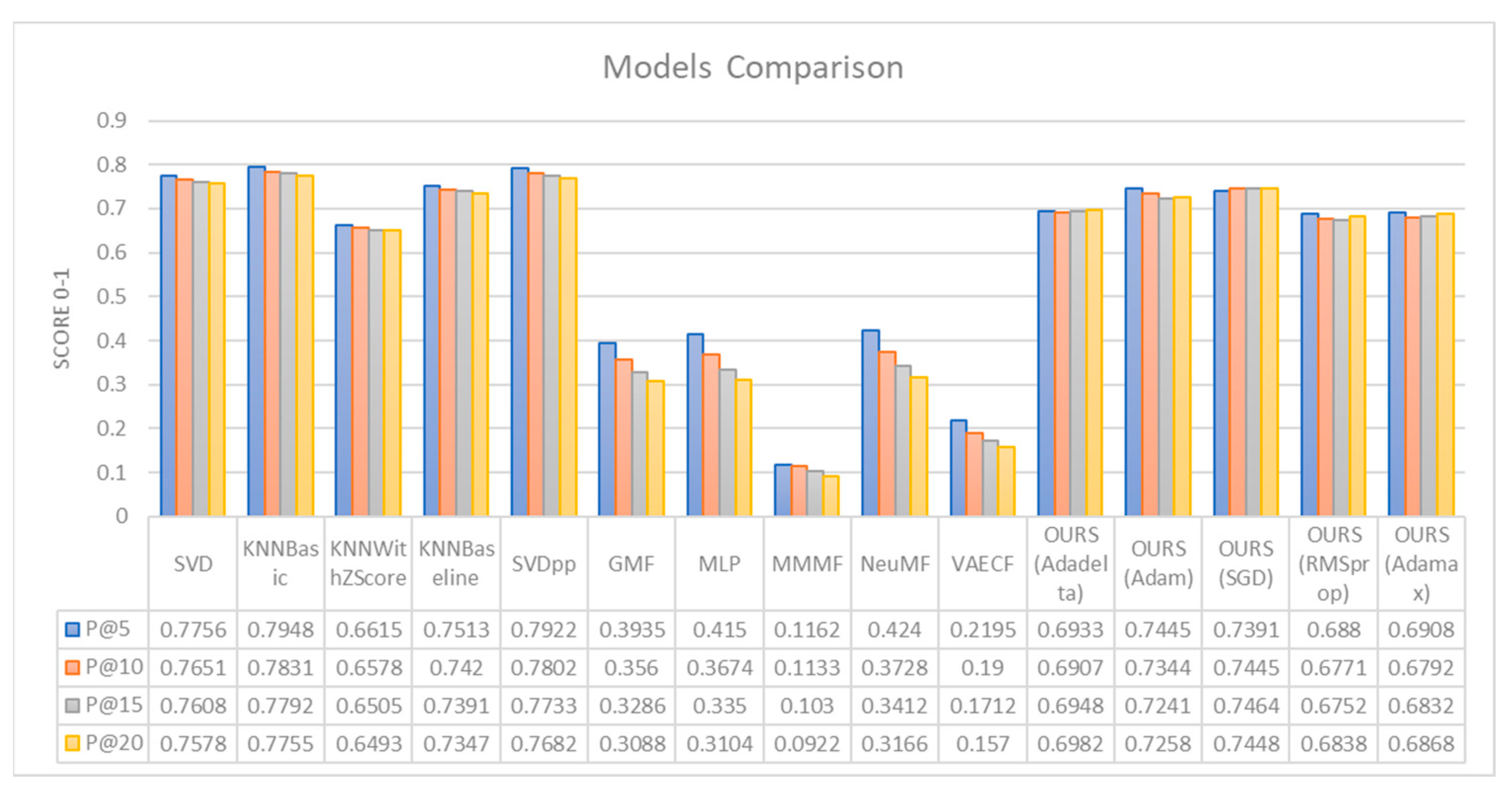
Experimental results demonstrate the efficacy of the proposed approach in comparison to baseline methods. Table 1 evaluates how many of the top-k recommendations are relevant and the recommendation result analysis. The current study selects various $k$ evaluations. A higher P@k value indicates a greater number of relevant recommendations of the top-k items, making the model more effective in its suggestions. To provide convenience analysis, the study divides the results into three parts, including Surprise, Cornac, and the proposed model from our side. In the first part, we discuss the Surprise library; in the second, we analyze performance using Cornac; and, finally, we present the results from our proposed model. Table 1 presents a comparative analysis of the recommendation system from various library perspectives.

Table 1. Performance Results of Recommendation Models.

Models	P@5	P@10	P@15	P@20
SVD	0.7756	0.7651	0.7608	0.7578
KNNBasic	0.7948	0.7831	0.7792	0.7755
KNNWithZScore	0.6615	0.6578	0.6505	0.6493
KNNBaseline	0.7513	0.7420	0.7391	0.7347
SVDpp	0.7922	0.7802	0.7733	0.7682
GMF	0.3935	0.3560	0.3286	0.3088
MLP	0.4150	0.3674	0.3350	0.3104
MMMF	0.1162	0.1133	0.1030	0.0922
NeuMF	0.4240	0.3728	0.3412	0.3166
VAECF	0.2195	0.1900	0.1712	0.1570
OURS (Adadelta)	0.6933	0.6907	0.6948	0.6982
OURS (Adam)	0.7445	0.7344	0.7241	0.7258
OURS (SGD)	0.7391	0.7445	0.7464	0.7448
OURS (RMSprop)	0.6880	0.6771	0.6752	0.6838
OURS (Adamax)	0.6908	0.6792	0.6832	0.6868

Figure 4 displays the visualization results from our implementation techniques. The study shows the recommendation performance between the benchmark models and our models. The graph includes a variety of models, such as SVD, k-Nearest Neighbors (KNN)-based models with different optimizations, Singular Value Decomposition++ (SVDpp), Generalized Matrix Factorization (GMF), Multi-Layer Perceptron (MLP), and others, including several variations of a model denoted as “OURS”, with different optimizations like AdaGrad, SGD, RMSprop, and Adamax. We conduct a test of metrics evaluation score for each model at different levels of k (5, 10, 15, 20), which evaluates the models on how well they predict the top 5, 10, 15, and 20 items on a recommendation list. The scores are typically between 0 and 1, with 1 being a perfect score.

Figure 4. Comparison results from our proposed model with benchmark models.

First, we introduce the evaluation model from our work. Among the five optimizer techniques that are used with the system, OURS (Adam and SGD) yields the best result among OURS (Adadelta, Adamax, RMSprop). The Adam optimizer is the model that performs best at P@5, while the SGD optimizer leads at P@10, P@15, and P@20 (0.7445, 0.7464, 0.7448). The lowest model within the proposed system is OURS (RMSprop). It shows the lowest performance across all the k values (0.6880, 0.6771, 0.6752, 0.6838). The Adadelta (0.6933, 0.6907, 0.6948, 0.6982) and Adamax (0.6908, 0.6792, 0.6832, 0.6868) optimizers perform better than RMSprop but do not outperform Adam and SGD.

Next, we compare them with other benchmark models. Among all comparison models, KNNBasic achieves the highest precision values across all k values (0.7948, 0.7831, 0.7792, 0.7755), indicating that it is the best-performing model. The second-best model with precision values of 0.7922, 0.7802, 0.7733, 0.7682, SVD shows consistent performance with a slight decline as k increases (0.7756, 0.7651, 0.7608, 0.7578). KNNBaseline performs slightly worse than SVD (0.7513, 0.7420, 0.7391, 0.7347). KNNWithZScore has the lowest performance in the Surprise library (0.6615, 0.6578, 0.6505, 0.6493).

The benchmark models from the Cornac library demonstrates the worst performance. Nevertheless, the library achieves its peak performance when it reaches a certain threshold of user interactions or when it is configured with optimal parameters, which are determined by the specific application context or user requirements. Among the Cornac models, NeuMF has the best precision scores of 0.4240, 0.3728, 0.3412, and 0.3166. The MLP model ranks second in the Cornac library, with performance metrics of 0.4150, 0.3674, 0.3350, and 0.3104. The performance of MMMF is the lowest with values of 0.1162, 0.1133, 0.1030, and 0.0922. Both GMF and VAECF exhibit reasonable results, though VAECF performs better.

While our proposed models do not exceed the performance of the Surprise library, they do surpass the models of the Cornac library. We firmly assert that our models provide a diverse range of learning experiences according to their ability to learn dynamically, as opposed to the static nature of the models in the Surprise collection. Many performance results reflect a decrease with each subsequent increase in k, which is a prevalent pattern observed in recommendation systems.

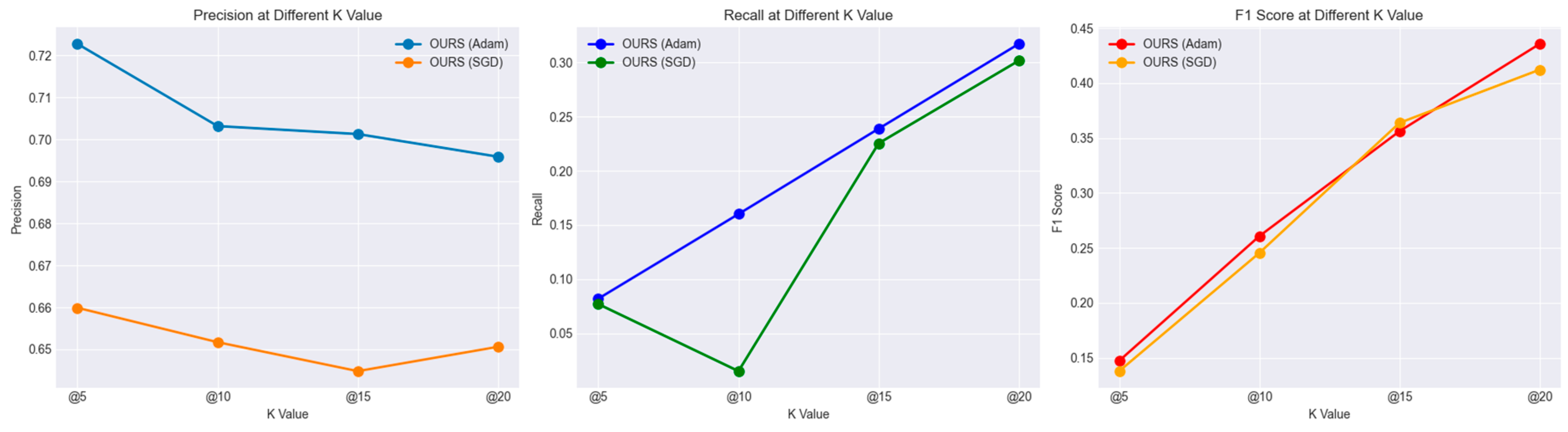
Figure 5 introduces additional metrics for evaluating our performance, including Precision, Recall, and the F1 score. According to the results shown in Figure 4, OURS (using Adam and SGD) yields the best results among the variations of OURS (including Adadelta, Adamax, RMSprop). Thus, we illustrate the performance of recommendation systems optimized with Adam and SGD across various k values, based on three different metrics: Precision, Recall, and F1 Score. The Precision graph indicates that the performance of both optimizers decreases slightly as k increases. SGD starts off stronger at k = 5, but Adam shows more consistency across all k values. The Recall graph shows more variability. Adam starts lower than SGD at k = 5, surpasses it at k = 10, then falls below again at k = 15, with both lines finally converging at k = 20. To find the balance between precision and recall, we turn to the F1 score graph, which combines both metrics. This graph shows a consistent increase as k increases. Both Adam and SGD perform similarly at each k value, though Adam starts off slightly better at k = 5 and finishes similarly at k = 20. This visualization suggests that the performance of the recommendation system varies depending on the chosen metric and the value of k. Such an analysis is important to determine which optimizer to use depending on whether the goal is to maximize precision, recall, or a balance of both (F1 score). Precision measures how many of those recommended items are actually relevant or interesting to the user. For example, if a system recommends 10 movies to a user (k = 10), and 9 out of these 10 are movies the user would like, then the precision at 10 is 0.9.

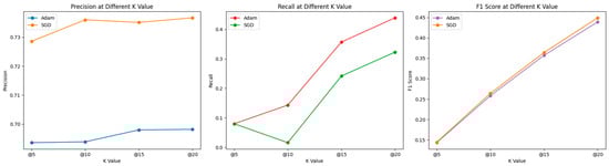
Figure 5. Comparative Analysis of Adam and SGD Optimizers Across Different K Values for Precision, Recall, and F1 Score Metrics.

Recall measures how many of the relevant items you managed to find with your recommendation. A high recall means that the system retrieved most of the relevant items but does not care about how many irrelevant items were also recommended. For example, if there are 20 movies that the user would like, and the system recommends 10 movies, out of which 5 are relevant, then the recall at 10 is 0.25. Typically, there is a trade-off between precision and recall. If we recommend many items (increasing k), it is more likely to include all the relevant ones (increasing recall), but it is also likely to include more irrelevant ones (decreasing precision). Conversely, if we recommend fewer items, we might miss some relevant ones (decreasing recall) but increase the likelihood that the recommended items are relevant (increasing precision).

5. Ablation Study

To enhance the significance and benefits of our proposed recommendation framework, this section introduces an ablation study. We conducted four ablation experiments against our current model setup. In the first ablation experiment, we removed the dropout layers from the networks. The second ablation involved changing the learning rate to both higher and lower values. The third ablation attempted to use a smaller replay buffer, while the fourth ablation altered the method of reward calculation. For each of these, the model was retrained and evaluated using the defined metrics (Precision, Recall, F1 Score).

• Ablation—Alters the method of reward calculation.

The reward structure is a key factor in shaping the policy learned by the agent, as it directly influences what the model perceives as desirable outcomes. The current reward of our setup is the normalization of user ratings into rewards. To define new reward calculation methods, we define the new binary reward structure as follows: Positive Interaction (Reward = 1): This defines what constitutes a positive interaction. Typically, this could be user ratings above a certain threshold (e.g., ratings of 4 or 5 out of 5). Negative or Neutral Interaction (Reward = 0): This is defined as what constitutes a negative or neutral interaction, e.g., ratings below your chosen threshold. We have chosen to display Adam and SGD due to their high performance relative to other optimization techniques, as indicated by the outperforming results in Table 1. We will then retrain the model, maintaining all other settings for consistency.

o

Potential Outcomes and Interpretation:

▪

Decreased Performance: The new reward system does not outperform our current models. It suggests that the new reward structure is either too simplistic and not capturing the nuances of user preferences, or overly complex, confusing the learning process. The model aims to capture only the user binary rate as 1 or 0. In addition, that is the reason for reducing the performance of the recommendation metrics. The new reward structure aligns better with the desired outcomes of our model, which uses Adam optimizers rather than the one with SGD. But this binary reward does not seem to perform well, especially when the metric k becomes bigger, as shown in Figure 6.

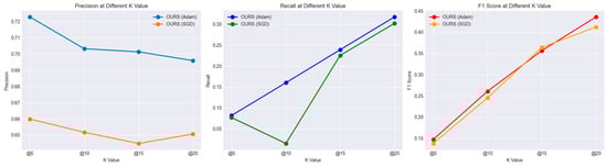Figure 6. Comparison of Results Using the Newly Defined Binary Reward Structure in the Ablation Study.

6. Conclusions

Our study presents an innovative method in movie recommendation systems, characterized by the deliberate combination of deep reinforcement learning (DRL) and collaborative filtering (CF). This approach harnesses the flexibility of deep reinforcement learning (DRL) and the dependability of classic collaborative filtering (CF), resulting in a recommendation system that is more resilient and efficient.

The actor–critic technique in DRL is crucial to our approach as it combines policy-based and value-based tactics, possibly improving the recommendation process. In addition, the use of the Deep Deterministic Policy Gradient (DDPG) facilitates ongoing and complex user–movie interactions, promoting a system that is both adaptable and responsive to individual user preferences. Singular value decomposition (SVD) is applied to perform matrix factorization in collaborative filtering (CF), demonstrating further advancements in innovation. This enables the retrieval of intricate embeddings that encompass crucial user and movie characteristics, leading to a substantial enhancement in suggestion precision and personalization. Our approach incorporates an adaptive maximum state representation obtained through singular value decomposition (SVD), dynamically adapting to user preferences, resulting in suggestions that are both more accurate and personalized. The solution tackles significant industrial obstacles such as the capacity to handle large amounts of data and reducing the complexity of dimensions by employing the strategic use of singular value decomposition (SVD). Furthermore, the intrinsic adaptability of DRL is utilized to improve the process of exploring and exploiting recommendations. Crucially, our method demonstrates the potential to address the cold-start issue by offering well-informed recommendations despite having minimal user data. The efficacy of our integrated method is shown by its capacity to find the most favorable cumulative reward, resulting in a significant improvement in the overall performance of the system. This combination of sophisticated methodologies not only establishes a fresh benchmark in recommendation systems but also opens up possibilities for future advancements in this domain.

References

- Kim, H.M.; Ghiasi, B.; Spear, M.; Laskowski, M.; Li, J. Online serendipity: The case for curated recommender systems. Bus. Horiz. 2017, 60, 613–620. [Google Scholar] [CrossRef]
- Thorat, P.B.; Goudar, R.M.; Barve, S. Survey on collaborative filtering, content-based filtering and hybrid recommendation system. Int. J. Comput. Appl. 2015, 110, 31–36. [Google Scholar]
- Ferreira, D.; Silva, S.; Abelha, A.; Machado, J. Recommendation system using autoencoders. Appl. Sci. 2020, 10, 5510. [Google Scholar] [CrossRef]
- Elguea, Í.; Arana-Arexolaleiba, N.; Serrano Muñoz, A. A review on reinforcement learning for contact-rich robotic manipulation tasks. Robot. Comput.-Integr. Manuf. 2023, 81, 102517. [Google Scholar] [CrossRef]
- Li, M.; Wang, Z. Deep learning for high-dimensional reliability analysis. Mech. Syst. Signal Process. 2020, 139, 106399. [Google Scholar] [CrossRef]
- Kulkarni, T.D.; Narasimhan, K.; Saeedi, A.; Tenenbaum, J. Hierarchical deep reinforcement learning: Integrating temporal abstraction and intrinsic motivation. Adv. Neural Inf. Process. Syst. 2016, 29, 3682–3690. [Google Scholar]
- Harper, F.M.; Konstan, J.A. The movielens datasets: History and context. Acm Trans. Interact. Intell. Syst. 2015, 5, 1–19. [Google Scholar] [CrossRef]
- Vilakone, P.; Xinchang, K.; Park, D.S. Personalized movie recommendation system combining data mining with the k-clique method. J. Inf. Process. Syst. 2019, 15, 1141–1155. [Google Scholar]
- Peng, S.; Park, D.S.; Kim, D.Y.; Yang, Y.; Siet, S.; Ugli SI, R.; Lee, H. A Modern Recommendation System Survey in the Big Data Era. In International Conference on Computer Science and Its Applications and the International Conference on Ubiquitous Information Technologies and Applications; Springer Nature Singapore: Singapore, 2022; pp. 577–582. [Google Scholar]
- Koren, Y.; Rendle, S.; Bell, R. Advances in collaborative filtering. In Recommender Systems Handbook; Springer: New York, NY, USA, 2021; pp. 91–142. [Google Scholar]
- Goldberg, D.; Nichols, D.; Oki, B.M.; Terry, D. Using collaborative filtering to weave an information tapestry. Commun. ACM 1992, 35, 61–70. [Google Scholar] [CrossRef]
- Koren, Y.; Bell, R.; Volinsky, C. Matrix factorization techniques for recommender systems. Computer 2009, 42, 30–37. [Google Scholar] [CrossRef]
- Liang, D.; Altosaar, J.; Charlin, L.; Blei, D.M. Factorization meets the item embedding: Regularizing matrix factorization with item co-occurrence. In Proceedings of the 10th ACM Conference on Recommender Systems, Boston, MA, USA, 15–19 September 2016; pp. 59–66. [Google Scholar]
- Tran, T.; Lee, K.; Liao, Y.; Lee, D. Regularizing matrix factorization with user and item embeddings for recommendation. In Proceedings of the 27th ACM International Conference on Information and Knowledge Management, Torino, Italy, 22–26 October 2018; pp. 687–696. [Google Scholar]
- Deldjoo, Y.; Dacrema, M.F.; Constantin, M.G.; Eghbal-Zadeh, H.; Cereda, S.; Schedl, M.; Ionescu, B.; Cremonesi, P. Movie genome: Alleviating new item cold start in movie recommendation. User Model. User-Adapt. Interact. 2019, 29, 291–343. [Google Scholar] [CrossRef]
- Xinchang, K.; Vilakone, P.; Park, D.S. Movie recommendation algorithm using social network analysis to alleviate cold-start problem. J. Inf. Process. Syst. 2019, 15, 616–631. [Google Scholar]
- Vilakone, P.; Park, D.S.; Xinchang, K.; Hao, F. An efficient movie recommendation algorithm based on improved k-clique. Hum.-Centric Comput. Inf. Sci. 2018, 8, 38. [Google Scholar] [CrossRef]
- Van Meteren, R.; Van Someren, M. Using content-based filtering for recommendation. In Proceedings of the Machine Learning in the New Information Age: MLnet/ECML2000 Workshop, Barcelona, Spain, 30 May 2000; Volume 30, pp. 47–56. [Google Scholar]
- Bogdanov, D.; Haro, M.; Fuhrmann, F.; Xambó, A.; Gómez, E.; Herrera, P. Semantic audio content-based music recommendation and visualization based on user preference examples. Inf. Process. Manag. 2013, 49, 13–33. [Google Scholar] [CrossRef]
- Li, L.; Wang, D.; Li, T.; Knox, D.; Padmanabhan, B. Scene: A scalable two-stage personalized news recommendation system. In Proceedings of the 34th International ACM SIGIR Conference on Research and Development in Information Retrieval, Beijing, China, 24–28 July 2011; pp. 125–134. [Google Scholar]
- Tian, Y.; Zheng, B.; Wang, Y.; Zhang, Y.; Wu, Q. College library personalized recommendation system based on hybrid recommendation algorithm. Procedia CIRP 2019, 83, 490–494. [Google Scholar] [CrossRef]
- Wang, H.; Wang, N.; Yeung, D.Y. Collaborative deep learning for recommender systems. In Proceedings of the 21th ACM SIGKDD International Conference on Knowledge Discovery and Data Mining, Sydney, NSW, Australia, 10–13 August 2014; pp. 1235–1244. [Google Scholar]
- Zhang, S.; Yao, L.; Sun, A.; Tay, Y. Deep learning based recommender system: A survey and new perspectives. ACM Comput. Surv. (CSUR) 2019, 52, 1–38. [Google Scholar] [CrossRef]
- Cheng, H.T.; Koc, L.; Harmsen, J.; Shaked, T.; Chandra, T.; Aradhye, H.; Anderson, G.; Corrado, G.; Chai, W.; Ispir, M.; et al. Wide & deep learning for recommender systems. In Proceedings of the 1st Workshop on Deep Learning for Recommender Systems, Boston, MA, USA, 15 September 2016; pp. 7–10. [Google Scholar]
- Naumov, M.; Mudigere, D.; Shi, H.J.M.; Huang, J.; Sundaraman, N.; Park, J.; Wang, X.; Gupta, U.; Wu, C.-J.; Azzolini, A.G.; et al. Deep learning recommendation model for personalization and recommendation systems. arXiv 2019, arXiv:1901.02103. [Google Scholar]
- Li, Z.; Shi, L.; Cristea, A.I.; Zhou, Y. A survey of collaborative reinforcement learning: Interactive methods and design patterns. In Proceedings of the 2021 ACM Designing Interactive Systems Conference, Virtual, 28 June–2 July 2021; pp. 1579–1590. [Google Scholar]
- Zhao, X.; Xia, L.; Zou, L.; Yin, D.; Tang, J. Toward simulating environments in reinforcement learning based recommendations. arXiv 2019, arXiv:1906.11462. [Google Scholar]
- Deliu, N. Reinforcement learning for sequential decision making in population research. Qual. Quant. 2023, 1–24. [Google Scholar] [CrossRef]
- Zou, L.; Xia, L.; Ding, Z.; Song, J.; Liu, W.; Yin, D. Reinforcement learning to optimize long-term user engagement in recommender systems. In Proceedings of the 25th ACM SIGKDD International Conference on Knowledge Discovery & Data Mining, Anchorage, AK, USA, 4–8 August 2019; pp. 2810–2818. [Google Scholar]
- Mlika, F.; Karoui, W. Proposed model to intelligent recommendation system based on Markov chains and grouping of genres. Procedia Comput. Sci. 2020, 176, 868–877. [Google Scholar] [CrossRef]
- Arulkumaran, K.; Deisenroth, M.P.; Brundage, M.; Bharath, A.A. Deep reinforcement learning: A brief survey. IEEE Signal Process. Mag. 2017, 34, 26–38. [Google Scholar] [CrossRef]
- Hug, N. Surprise: A Python library for recommender systems. J. Open Source Softw. 2020, 5, 2174. [Google Scholar] [CrossRef]
- Salah, A.; Truong, Q.T.; Lauw, H.W. Cornac: A comparative framework for multimodal recommender systems. J. Mach. Learn. Res. 2020, 21, 3803–3807. [Google Scholar]
Disclaimer/Publisher’s Note: The statements, opinions and data contained in all publications are solely those of the individual author(s) and contributor(s) and not of MDPI and/or the editor(s). MDPI and/or the editor(s) disclaim responsibility for any injury to people or property resulting from any ideas, methods, instructions or products referred to in the content. |
© 2024 by the authors. Licensee MDPI, Basel, Switzerland. This article is an open access article distributed under the terms and conditions of the Creative Commons Attribution (CC BY) license (https://creativecommons.org/licenses/by/4.0/).