Optimized Design of Pipe Elbows for Erosion Wear

Abstract

Multiphase flows are widely used to transport solid–liquid mixtures in oil and gas fields. The pipeline structures used can suffer damage from the high-pressure sand-carrying fracturing fluid, causing erosion and wear failures in the engineering field. In this work, an erosion model that considers particle turbulent kinetic energy and the effect of the design’s structural parameters on the erosion wear of spatial pipe structures is established using computational fluid dynamics (CFD). Structural parameters such as the bending diameter ratio, bending angle and spatial angle are discussed, and the location and degree of each parameter with regard to the erosion rate are obtained. The results show that the included angle of the pipe elbow has the greatest influence on erosion wear among the structural parameters. Several typical anti-erosion optimization models are compared and analysed, and a corrugated anti-erosion structure based on a bionic structure is further proposed. It is found that the anti-erosion performance of the T-type blind long header pipe is better in terms of the numerical value of the erosion rate, while for the erosion cloud diagram, the anti-erosion performance of the corrugated structure is superior. Finally, some suggestions for the application of the anti-erosion structure in the engineering field are given, and technical support is provided for the anti-erosion structure design and practical application of space pipeline systems in the future.

1. Introduction

Oil is an important strategic resource that plays a key role in all sectors of our industry as well as in national defence construction. In the extraction process, the use of high-pressure and high-viscosity fracturing fluids can increase oil and gas production. Pipes are an important component of fracturing a unit. As the sand-carrying fracturing fluid is forced to turn in the pipeline many times during an operation, the pipeline is subjected to severe erosion and wear. At the same time, because of the influence of the external environment, it is highly prone to failure, and the stability of the fracturing unit can be seriously affected.

In recent years, many scholars studying the elbow erosion wear problem have carried out extensive research. Mills [1] mentioned that there is a critical value in terms of sand particle diameter in the erosion and wear process. Throneberry [2] and Kesana [3] investigated different sand particle sizes by changing the liquid phase and flow rate to study the law between different sand grain sizes and the erosive wear rate. Parsi [4] conducted sand erosive wear experiments on vertical–horizontal elbows using a new ultrasonic device. By varying fluid factors such as the flow rate, grain size and viscosity, it was found that vertical–horizontal elbows suffered from more erosion wear than horizontal–horizontal elbows. For the erosion wear model, Chen [5] studied the relationship between bends and plugged tees on erosion and wear based on the erosion model of a liquid and solid two-phase flow and analysed the trajectory of particles and the shape of the erosion area using the Grant and Tabakoff [6] model of particles impacting on walls. Mazumder [7] carried out an experimental study on the erosion characteristics of single-phase and multiphase flows at different flow rates and verified that the maximum erosion and wear locations are different for different liquid flow directions and liquid phase types. Pereira [8] and Solnordal [9] found that the erosion pattern at the bend is V-shaped, which is mainly due to the friction between the solid particles and the wall. For different numerical simulation methods, Wood [10] studied liquid phase flow law and particle collision in different guided bends, analysing the incidence angle and velocity of the particle impact on walls using the Hashish [11] erosion model, and found that the maximum erosion location is in a particular area. In another study [12], the erosion and wear situation was calculated in bends with different bend-to-diameter ratios using numerical simulation; the results were compared with experiments, and it was found that the results were basically the same. For the (CFD)-based simulation method, Zahedi [13] used two different numerical simulation methods to analyse the different medium flows in the bend, with the results showing that the stability of the different models varies under different working conditions, and the computation time of the models is much longer. Zhang [14] verified the effectiveness of the computational fluid dynamics (CFD)-based simulation method in simulating and analysing the particle collision information in the pipe elbow. Zhang [15] fur ther verified the feasibility of CFD-based erosion and wear prediction by simulating different geometries, liquid flow rates and particle diameters for the pipe, showing that reasonable meshing, turbulence model selection and wall collision function selection are the key factors to achieving good results in simulation analysis and prediction. Using experimental and simulation methods, Peng [16] analysed the effects of different pipe diameters and sand characteristics on the erosion wear of elbows, and in another study, used two erosion models to investigate the erosive wear of solid particles on elbows in dispersed vesicular, annular and segmental plug flows, finding that the experimental data were closer to the simulation data. In summary, there is a lack of research on the influence of structural parameters on erosion wear. At the same time, there is relatively little research on improving the overall corrosion resistance of pipeline structures and extending their service life.

In our previous study [17], the effects of different fluid parameters and structural parameters of liquid–solid two-phase flow on the erosion wear of a pipeline structure were discussed. The maximum erosion wear location of the bend was well predicted, providing theoretical guidance for hazard prevention in engineering practice. In this study, based on the design of structural parameters, the study of pipe elbow erosion and the influence of erosion wear law, we analyse structural parameters such as the bend diameter ratio, bending angle and space angle at the bend. We also explore the change rule of erosion wear location and erosion wear degree based on the numerical simulation research method. A method for optimal design and bellows design is presented in this paper, providing a reference for further pipe design and optimization.

2. Numerical Analysis of the Erosion Model

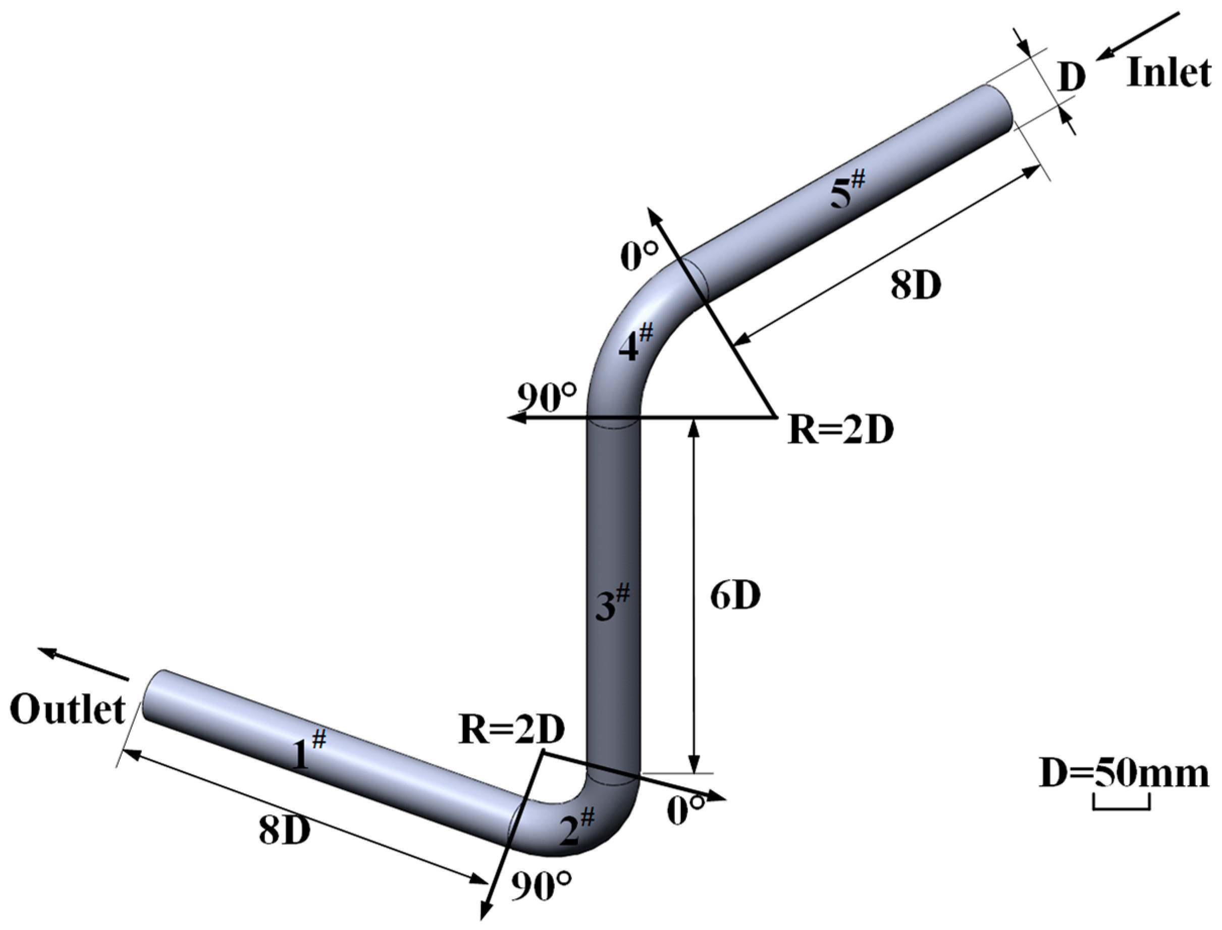
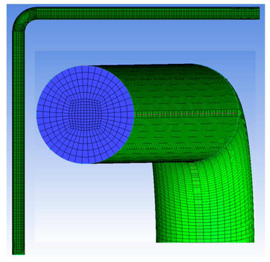
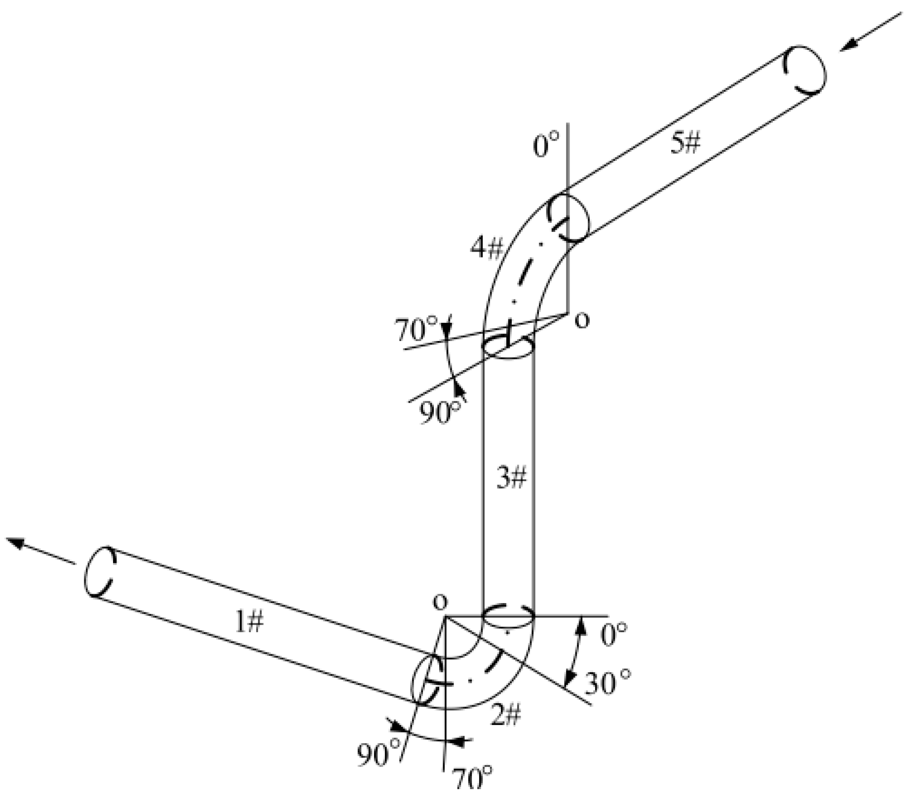
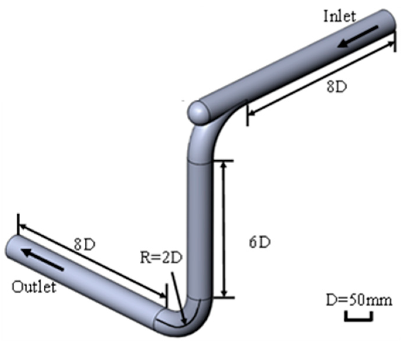
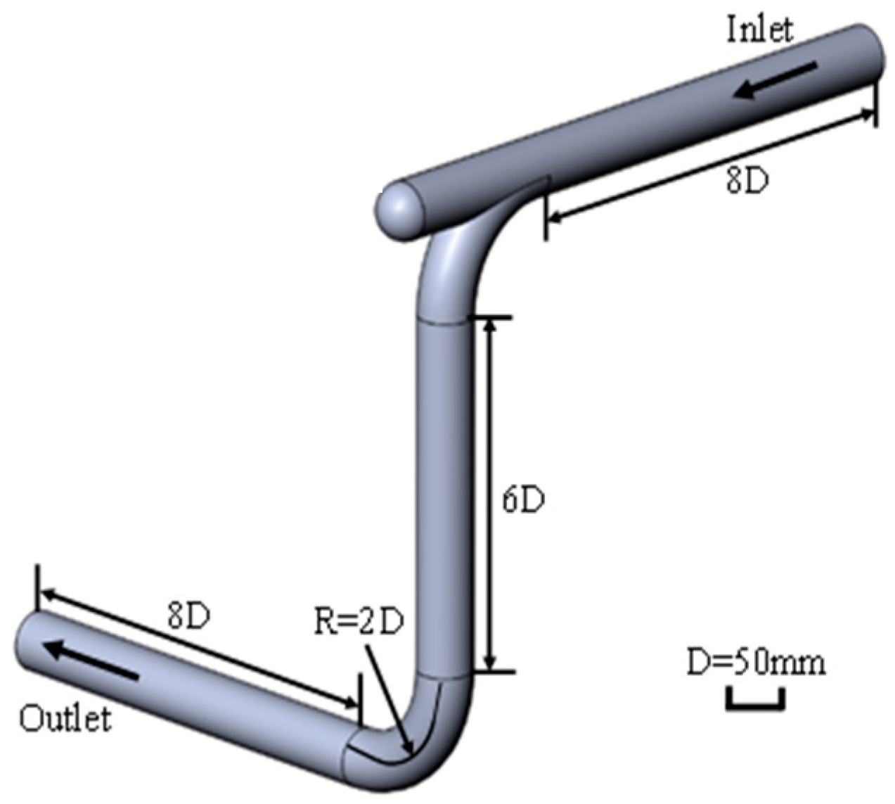
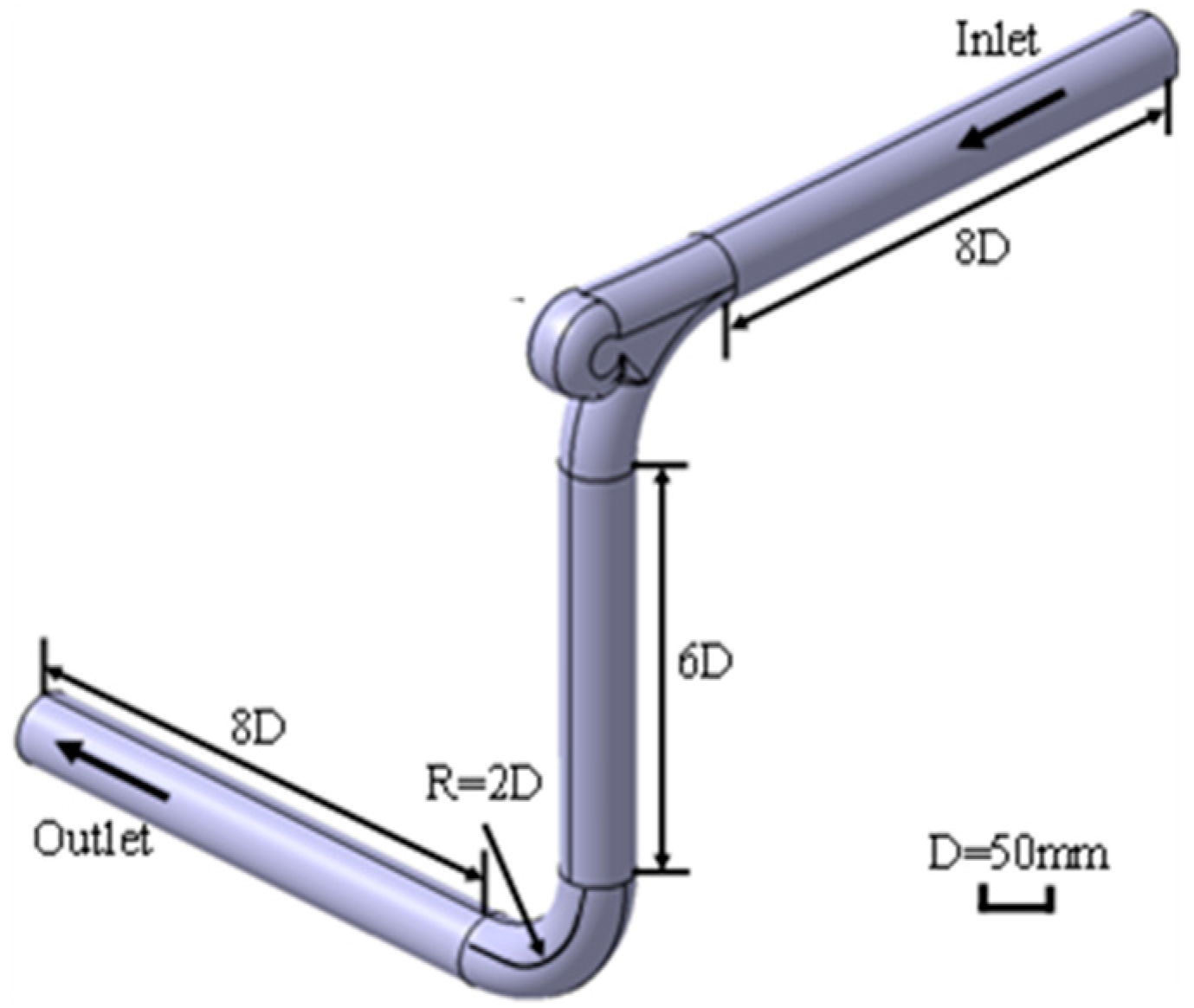
2.1. Pipe Parameters and Mesh Segmentation

In this paper, a typical pipe elbow is analysed as an example. The structural dimensions are shown in Figure 1, and the fracturing fluid parameters are shown in

Table 1. Fracturing fluid parameters.

Parameters of Fracturing Fluid	Symbol	Numerical	Units
Inner diameter	D	50	mm
Bend diameter ratio	R/D	2	——
Velocity	v	20	m/s
Particle diameter	d	0.00045	m
Density of sand	$\rho$	2650	kg/m3
Mass flow	mn	7	kg/s
Viscosity	ɳ	0.001	Pa·s

. The geometric model is a spatial anisotropic arrangement with a 90° angle. The upper right port is the inlet end, and the lower left port is the outlet end. The bend model consists of five segments: 1#, 3# and 5# are straight pipe segments, and 2# and 4# are 90° bend segments.

The mesh is divided as shown in Figure 2, where high-quality hexahedral elements are used in all components.

2.2. Theoretical Analysis of Erosion Wear

2.2.1. Computational Model

The flow of the fracturing fluid in the space pipe follows the conservation law of physics, resulting in the governing equation of the fluid as follows [18,19]:

(1)

Conservation of mass:

$$\frac{\partial \rho }{\partial t}+\frac{\partial }{\partial x_m}(\rho v_m)=0$$

(1)

(2)

Momentum equation:

$$\frac{\partial }{\partial t}(\rho v_m)+\frac{\partial }{\partial x_n}(\rho v_m{v}_n)=-\frac{\partial p}{\partial x_m}+\frac{\partial {\tau }_{mn}}{\partial c_n}+\rho g_n+V_m$$

(2)

$${\tau }_{mn}=\left[u(\frac{\partial v_m}{\partial x_n}+\frac{\partial v_n}{\partial x_m})\right]-\frac{2}{3}u\frac{\partial v_m}{\partial x_m}{\delta }_{mn}$$

(3)

(3)

Energy equation:

$$\frac{\partial }{\partial t}(\rho E)+\frac{\partial }{\partial x_m}\left[v_m(\rho E+p)\right]=\frac{\partial }{\partial x_m}\left[\lambda \frac{\partial T}{\partial x_m}-{\displaystyle \sum _{n^{\prime }}{h}_{n^{\prime }}{J}_{n^{\prime }}+v_n{\tau }_{mn}}\right]+S_{\epsilon }$$

(4)

Table 2. Parameters in the equation.

Parameters	Symbol	Units
Liquid phase density	ρ	kg/m3
Time	t	s
Thermal conductivity	λ	——
Stress tensor	${\tau }_{mn}$	Pa
Liquid phase velocity	v	m/s
Turbulent dissipation rate	E	m2/s3
Volume	Vm	m3
Pressure	p	MPa
Energy source	$S_{\epsilon }$	W/m3

explains the parameters in the equation.

2.2.2. Erosion Wear Model

The classical erosion wear model is selected and studied in this paper. The erosion wear rate model is defined as follows [20]:

$$R_{erosion}={\displaystyle \sum _{n=1}^N\frac{m_{n}C(d_n)f(\theta ){\omega }^{b(u)}}{A_{face}}}$$

(5)

where R_erosion is the rate of erosion wear; θ denotes the incidence angle; f(θ) represents the calculation function of the particle incidence angle; u stands for the particle velocity; and b(u) is the velocity coefficient of particles. The default value is 2.6. m_n is the particle mass flow rate, and C(d_n) represents a function related to particle properties, calculated according to particle shape, hardness and so on. The default value is 1.8 × 10⁻⁹. ω denotes the collision velocity of particles, and A_face is the area of the tube surface erosion calculation unit.

2.2.3. Turbulence Model Selection

The division of turbulence is based mainly on the size of the Reynolds number distinguished. For tube flow, a Reynolds number of over 2300 liquid flow is considered turbulence. The formula is as follows [21]:

$$R_{\epsilon }=\frac{\rho VD}{\mu }$$

(6)

where ρ is the fluid density; V represents the fluid velocity; D denotes the diameter of the pipeline; and μ is the fluid viscosity.

Turbulence is a very complex flow condition. There is currently no way to correctly describe its status. The accuracy of the Laminar model is not guaranteed. The relevant parameters of the k-omega model are difficult to obtain. The RNG k-ε model has the following form [22]:

$$\{\begin{array}{l}\frac{\partial (\rho k)}{\partial t}+\frac{\partial (\rho k{u}_i)}{\partial x_i}=\frac{\partial }{\partial x_i}\left[(\mu +\frac{{\mu }_t}{{\sigma }_k})\frac{\partial k}{\partial x_i}\right]+G_k-\rho \epsilon +S_k\\ \frac{\partial (\rho \epsilon )}{\partial t}+\frac{\partial (\rho k{u}_i)}{\partial x_i}=\frac{\partial }{\partial x_i}\left[(\mu +\frac{{\mu }_t}{{\sigma }_{\epsilon }})\frac{\partial k}{\partial x_j}\right]+G_{1\epsilon }\frac{\epsilon }{k}{G}_k-C_{2\epsilon }\rho \frac{{\epsilon }^2}{k}+S_{\epsilon }\end{array}$$

(7)

where $u_t=\rho C_u\frac{k^2}{\epsilon }$; k is the kinetic energy of liquid flow; µm represents the velocity of the liquid phase along the axis gradient; ρ denotes the density of the liquid phase; η stands for the viscosity of the liquid phase; G_k is a derivative of k; ε represents the dissipation of energy; xm and xn are the space coordinates; σ_k represents the Prandtl number corresponding to the dissipative active function, which is generally 1; and σ_ε is the Prandtl number corresponding to the power dissipated by turbulent kinetic energy, which is generally 1.2. In Fluent, the default Cu = 0.09, G_1ε = 1.44 and C_2ε = 1.92.

2.2.4. Wall Collision Recovery Coefficient

When sand collides with the inner wall of the pipeline, some energy is dissipated. As a result, the velocity of the particles after the collision is less than the initial velocity of the incident particle. The energy dissipation before and after sand impact is defined by the wall recovery coefficient. According to the recovery coefficient and the transfer and loss of energy, the equation can be seen in the following form:

$$\{\begin{array}{l}{\epsilon }_N=0.993-0.0307\theta +4.75\times {10}^{-4}{\theta }^2-2.61\times {10}^{-6}{\theta }^3\\ {\epsilon }_T=0.998-0.029\theta +6.43\times {10}^{-4}{\theta }^2-3.56\times {10}^{-6}{\theta }^3\end{array}$$

(8)

where θ is the impact angle of particles.

2.3. Boundary Condition Settings

The numerical simulation process on the software boundary conditions is set as follows: the turbulence model selection is the realizable k-ε turbulence model; the continuous phase is set to water; particles are set for the discrete phase; the inlet is defined as velocity inlet; the turbulence intensity and hydraulic diameter are set to the boundary settings—turbulence intensity is set to 5%, and the hydraulic diameter is used for the diameter of the pipe; the exit is defined as free-flowing; the wall conditions are set based on the DPM (discrete phase model); import and export are set to escape; the wall particle conditions are set to reflect; and the SIMPLE (semi-implicit method for pressure-linked equation) algorithm is used to solve the problem. The DPM is set; the inlet and outlet are set to escape; the wall particle condition is set to reflect; the SIMPLE algorithm is applied to solve the problem; the simulation process is set to calculate every five steps; and the outlet detection pressure value is set to converge at 10⁻⁵.

2.4. Validation of the Numerical Model Validity

Peng’s experimental tests are numerically modelled in this paper [16]. The liquid phase and discrete phase parameters are set up with the same conditions as the test. The maximum erosion rate and the maximum erosion position of the erosion wear are obtained with simulation and analysis. The experimental data in the literature are compared and analysed to verify the validity of the numerical model in this paper.

2.4.1. Calculation of Working Conditions

The liquid–solid two-phase flow conditions of the experimental data are used to verify the elbow erosion wear, with the specific experimental data shown in

Table 3. Specimen liquid–solid two-phase flow erosion experiment parameters.

	Numerical	Units
Speed	4.09	m/s
Diameter	300	µm
Density	2650	kg/m3
Mass flow rate	0.1027	kg/s
Density of material	7980	kg/m3

.

The velocity inlet was used by the pipe inlet. The liquid phase velocity v = 4 m/s, turbulence intensity and hydraulic diameter were chosen based on the turbulence parameters, and they were set to 5% and 0.04 m, respectively. The particle phase was set to escape at the inlet. The elbow exit was set to outflow, and the particle phase was set to capture at the exit. The particle diameter was 0.3 mm, and the mass flow rate was 0.1 kg/s.

2.4.2. Comparison of Numerical Simulation Erosion Models

The Zhang [17] erosion model as well as Forder’s wall bounce coefficients were used for simulation calculations. The maximum erosion rate cloud obtained with numerical simulation based on the experimental working condition parameters in

Table 4. Experimental data and numerical simulation data.

	Experimental Data from the Literature	Simulation Data from the Literature	Experimental Data from the Literature	Simulation Data from This Paper
Numerical (nm/s)	0.219	0.254	0.219	0.240
Inaccuracy	15.98%		9.59%

is shown in Figure 3.

As can be seen from Figure 3, the maximum erosion rate of the elbow is 1.45 × 10⁻⁸ kg/(m²·s). The maximum erosion location is at the outlet end of the 90° elbow and the straight pipe connection. From Figure 4, it can be seen that the maximum erosion thickness is 21.9 × 10⁻¹¹ m/s, and the erosion wear rate obtained from the simulation model verification in this paper is 0.254 nm/s.

The value of the error between the simulation results and the experimental data in this paper is 9.59%, which is smaller than the error between the numerical simulation and the experiment in the literature. This proves that the numerical model in this paper is closer to the experimental results. The existence of the error may be because the liquid phase flow in the experimental process is more complex, and the mutual collision between the particles and the impact of the angle of the particles are different. However, the overall error is less than 10%, which is credible.

3. Analysis of the Numerical Results

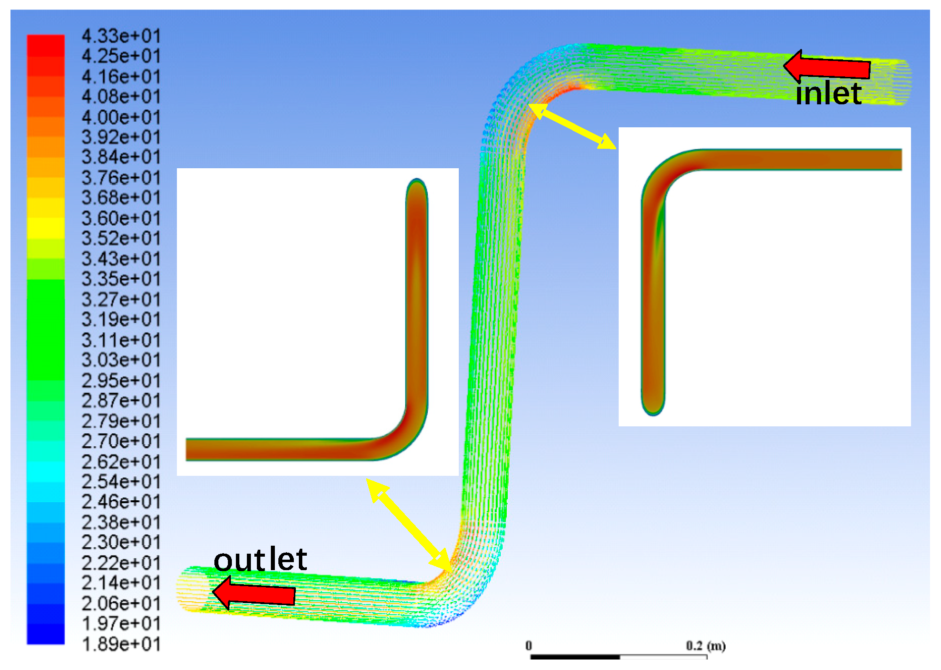
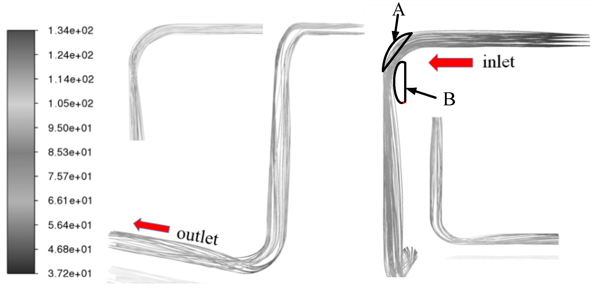
3.1. Liquid-Phase Flow Pattern

When the velocity of the liquid phase changes, the pressure of the liquid phase will change with it, and the magnitude of the change is the same, as shown in the figure.

As shown in Figure 5, because of the liquid flow in the pipeline, the “secondary flow” phenomenon occurs very easily, resulting in the fluid flowing through the elbow and the convex wall of the flow rate increasing, while the concave wall of the flow rate is slowed down by the obstruction of the velocity difference that is formed.

As shown in Figure 6, the pressure decreases from the inlet end to the outlet end along the direction of flow of the liquid phase. At the bend, the pressure value is inversely proportional to the velocity value, and the direction of the fluid is changed at the concave wall. This results in an increase in the fluid pressure and a decrease in the pressure at the convex wall as a result of the faster flow velocity.

As can be seen in Figure 7, in the straight pipe section, the linear motion is presented by the steady-state fluid carrying sand particles. At the elbow, the continuous phase is affected by the “secondary flow”, and the movement of sand particles at the elbow changes irregularly. At the inlet end of the elbow, the fracturing fluid is compressed because of the high pressure at the concave wall. At the convex wall, the flow rate is fast, the fracturing fluid is stretched and the vortex zone (A region) is formed at the concave wall; at the exit end of the bend, the fluid collision is folded back, and the vortex zone at the convex wall is formed due to the local pressure and velocity difference in the B region. At the 4# bend, a large number of sand particles are concentrated through the 90° wall of the bend outlet and adjacent to the straight pipe section. The flow state of sand particles is relatively stable after entering the 3# straight pipe section. A large number of sand particles flow along the outer wall vertically downward. In the flow through the 2# bend, a large number of sand particles hit the inlet end, and the front direction is changed. This results in the 2# bend section of the two vortex regions being moved forward, and the sand particles concentrated in the flow area changing in the bend under the joint influence of centrifugal force and flow velocity, creating an inward-rotating flow phenomenon in the exit end of the bend particle trajectory.

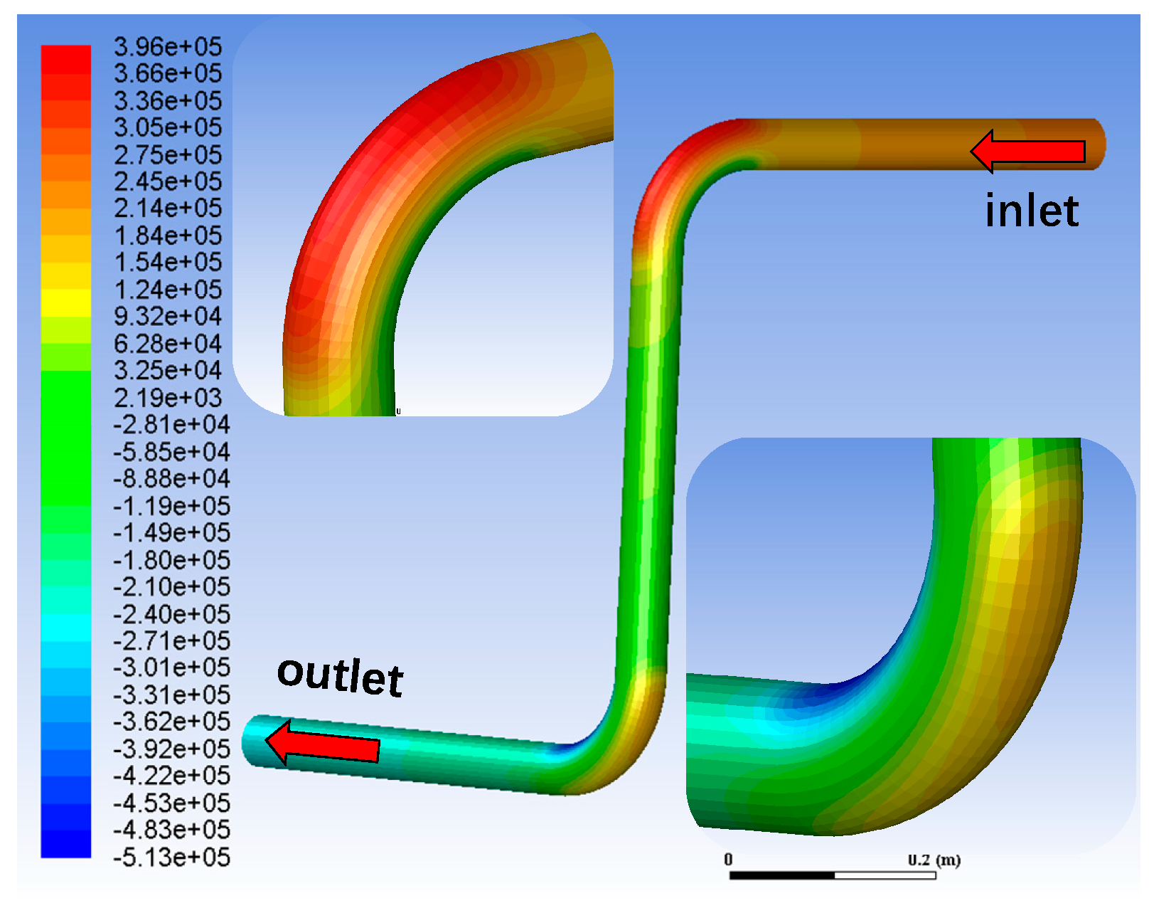
3.2. Characterization of Erosion and Wear

The discrete phase particle density was set to ρ = 2650 kg/m³, the particle size was set to 0.45 mm, the viscosity was set to 0.001 Pa·s and the flow rate was set to 20 m/s.

As illustrated in Figure 8, the fracturing fluid erosion of the pipe confluence occurs mainly in the two bent pipe areas of 2# and 4#. The bent pipe section is more easily eroded than the straight pipe section. At the bends, the sand particles are affected by centrifugal force and the local vortex zone, which makes the outer wall of the pipe confluence more likely to be impacted than the inner wall, resulting in serious erosion and wear.

As displayed in Figure 9, the 4# bend has no erosion phenomenon in the 0°~10° range, while the erosion intensity is the greatest in the position of 70°~90°. As the particles enter the bend section, the direction of fluid velocity is changed and is affected by the vortices in the A and B regions. The flow direction is shifted to the inside, and the wall surface of the bend is hit by a large number of particles positively. The position of 70°~90° has a large number of particles, the flow velocity is fast and the erosion and wear are intensified.

The main erosion and wear location of the 2# bend is located at 0°~30° and 70°~90° of the bend, and the particle trajectory reveals that a large number of sand particles fall vertically along the straight pipe section. The bend is affected by the centrifugal force of sand particles as well as gravity, and the wall surface of the bend within the range of 0°~30° is impacted, resulting in serious erosion at the inlet end of the bend. In addition, the “secondary flow” and the local vortex impact, part of the particles in the impact and then the fluid movement trend to the high angle position of the bend results in the 70°~90° position of the bend also appearing in the serious erosion area. However, the main erosion area of the 2# elbow is located on one side of the elbow centre axis section, rather than in the middle or evenly distributed on both sides. This is because the convex wall vortex region B causes the 4# elbow side of the outer wall to form a clear fluid extrusion surface, and most of the particles will be along the outer pipe wall down to the 2# elbow unilateral outer wall surface for shear effect, resulting in serious cutting wear. Moreover, because of the existence of a secondary flow vortex at the exit of the 2# elbow, the straight pipe section of the exit section will also produce a certain degree of erosion wear.

4. Analysis of the Influence of Structural Parameters on the Erosion and Wear of Pipe Elbows

In this section of the simulation, the flow rate is set to 5 m/s, the particle diameter is 0.45 mm, the mass flow rate is 0.2 kg/s, the viscosity is 0.001 Pa⋅s and the direction of gravity is vertically downward.

4.1. Influence of the Bending Diameter Ratio on the Erosion Wear of Pipe Elbows

In the actual layout of the project, the bend diameter ratio of the pipe is one of the important factors affecting the overall erosion and wear rate of the bend. The effect of the bending diameter ratio on erosion wear is shown in Figure 10.

The two arrangements changing the bending diameter ratio of the bend can be seen in Figure 11a. The maximum erosion rate is first decreased, then increased and gradually levelled off. However, it can be seen from erosion cloud diagram 1 that the maximum erosion location is changed. It can be seen that by changing the bend ratio at the inlet end when the bend ratio is less than 1.5, the maximum erosion location is at the bend near the inlet end. When the bend ratio is greater than 2, the maximum erosion location appears in the bend near the outlet end.

From Figure 11b, it can be seen that when the change in the bending diameter ratio of the bend is at the inlet end, and at the outlet end, there is a constant R/D = 2/1 of the bend, the inlet end of the bend at the maximum rate of erosion with the increase in the bending diameter ratio decreases; there is a bend ratio of 1.5~2 when the erosion rate is almost stable and unchanged; and there is a bend ratio of 2~3 when the rate of erosion and wear decreases slowly. Further, when there is a bend ratio of 0.5~1 at the exit end, the erosion and wear rate decline is larger; when there is a bend ratio of more than 1, the erosion and wear rate gradually increases and is gradually stable. When there is a bend ratio in the range of 1.5~2, the two sections of the bend erosion and wear rate close to the change is smooth.

Figure 11c shows that when the determined R/D = 2/1 of the bend is at the inlet end, and the change in the bending diameter ratio of the bend is at the outlet end, in the range of 0.5~1.5 of the small bending diameter ratio, the rate of erosion and wear rate changes, there is a bending diameter ratio of more than 1.5 and the maximum erosion and wear rate of the two bends is at the change in the flat. Therefore, the large bending diameter ratio of the bend causes a reduced erosion wear rate. In the project, the general selection of 1.5~2 for the bend ratio is more favourable.

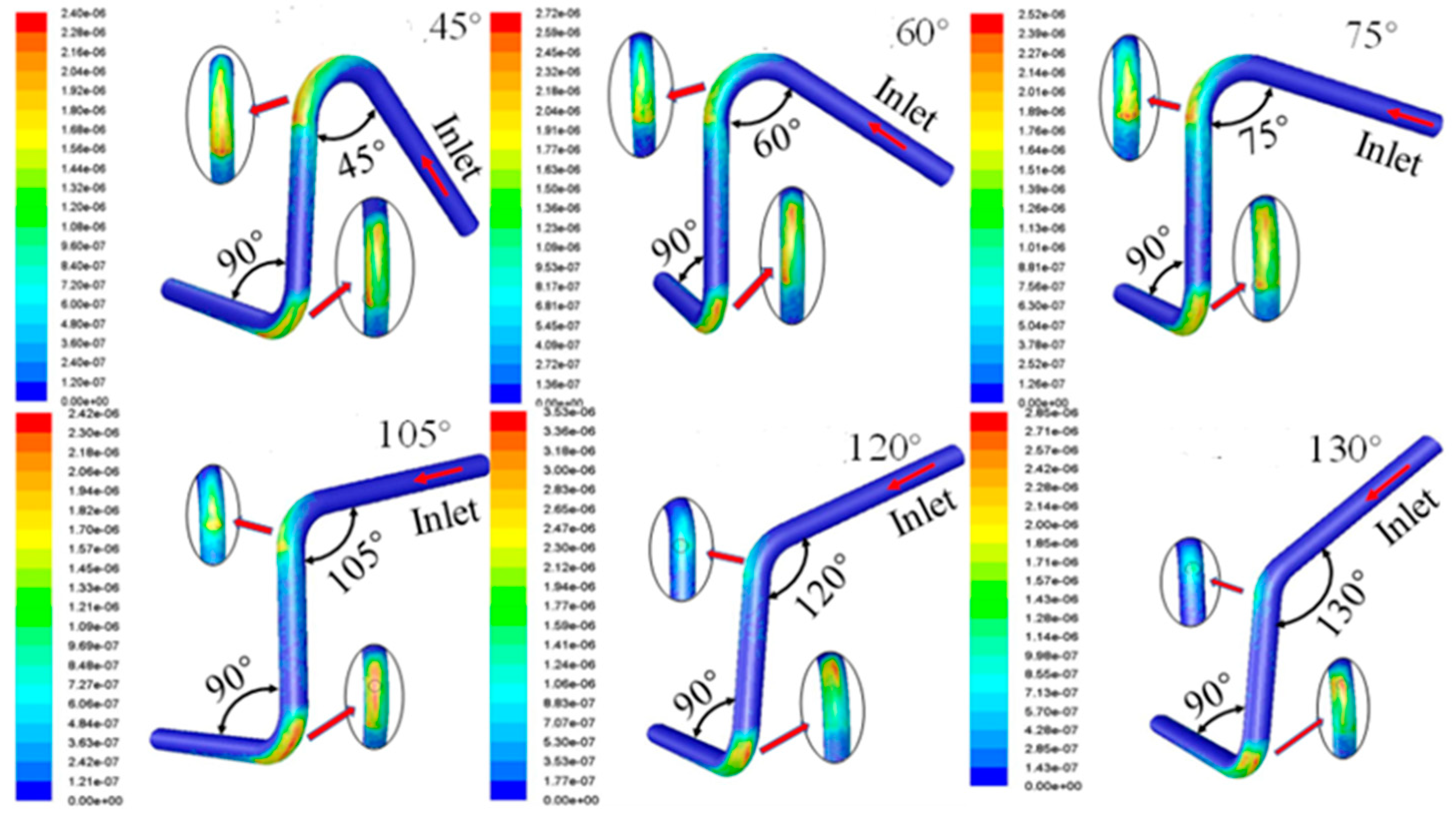
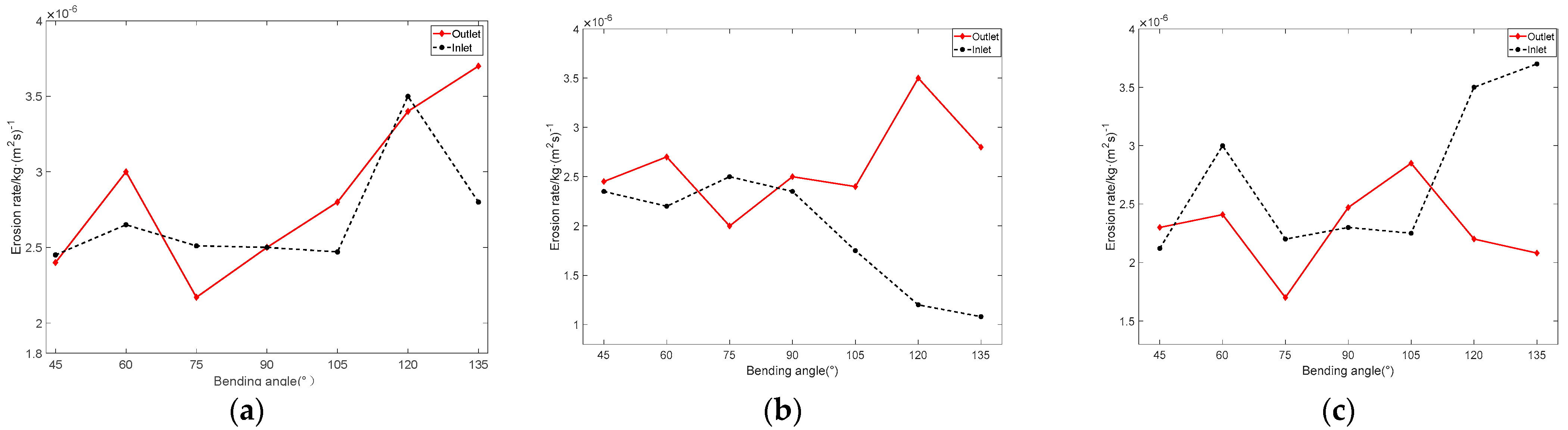
4.2. The Impact of the Bending Angle on the Pipe Elbow Erosion Wear

In the project, the bending angle of the elbow also affects the overall erosion wear rate of the elbow. The smaller the bend angle of the elbow, the stronger the constraint on small solid particles carried in the liquid phase, and the more violent the collision of the particles with the outer arch wall surface of the elbow. The effect of changing the bending angle at the inlet end on the erosion wear of pipe elbows is shown in the Figure 12.

As shown in Figure 13, with the increase in the bending angle of the bend near the exit end of the bend, the maximum erosion location is from the side of the bias to the position of the central axis of the bend. When the bending angle is less than 90°, both sections of the bend have more serious erosion areas. With the increase in the bending angle, the maximum erosion wear rate difference between the two sections of the bend increases. The inner wall of the bend with a smaller angle is subjected to an increased number of particle impacts, resulting in the existence of multiple erosion peaks in the bend.

As can be seen in Figure 14a, at the inlet end of the bend angle of 45°~105°, the overall maximum erosion wear rate of the bend changes gently. After exceeding 105°, the maximum erosion wear rate of the bend increases. When changing the bending angle of the bend at the outlet end, the maximum erosion wear rate of the bend increases gradually with the increase in the bending angle.

As illustrated in Figure 14b, when the bending angle of the inlet end of the bend increases from 45° to 90°, the change in the erosion and wear rate there is gentle. When there is an increase from 75° to 135° at the inlet end of the bend, the erosion and wear rate change with the increase in the bending angle and decline. The erosion wear rate at the outlet end elbow is less affected by the change in the angle of the inlet end elbow [23]. Around a certain value, the erosion rate fluctuates up and down. However, when the inlet end elbow angle exceeds 105°, the outlet end elbow erosion wear rate increases significantly. This is mainly because the increase in the bending angle of the inlet end bend results in a smoother flow of sand-carrying liquid. The sand particle incident angle decreases, and the degree of particle collision crushing is reduced, so that a large number of sand particles accumulate at the exit end of the bend, resulting in increased erosion and wear.

As can be seen from Figure 14c, when the bend angle is located downstream of the liquid-phase flow and the bend angle of the exit bend is 75°~105°, the change in the erosion and wear rate at the inlet end of the bend is small. After a bend angle of more than 105°, the inlet end of the elbow erosion and wear increased.

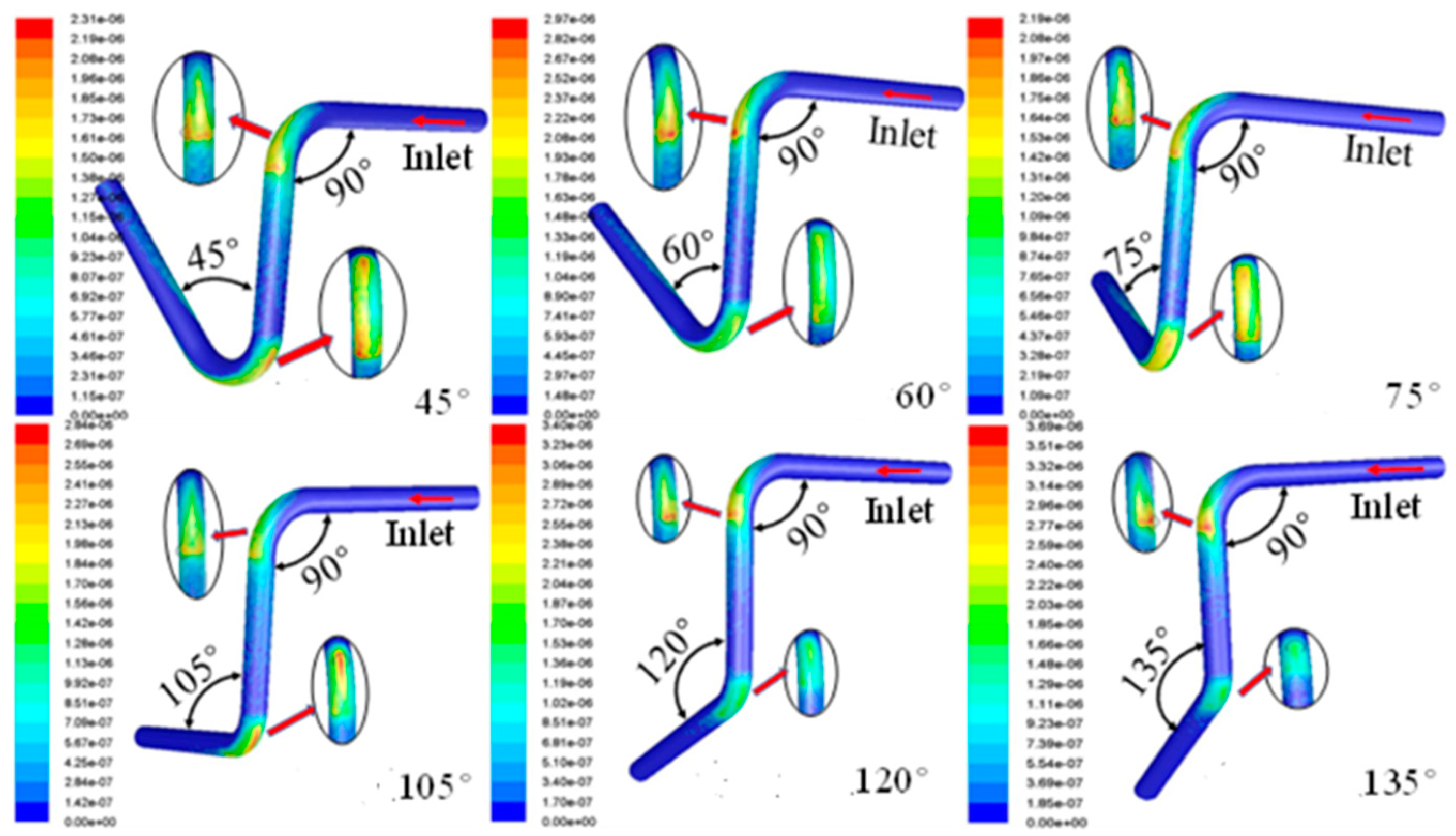
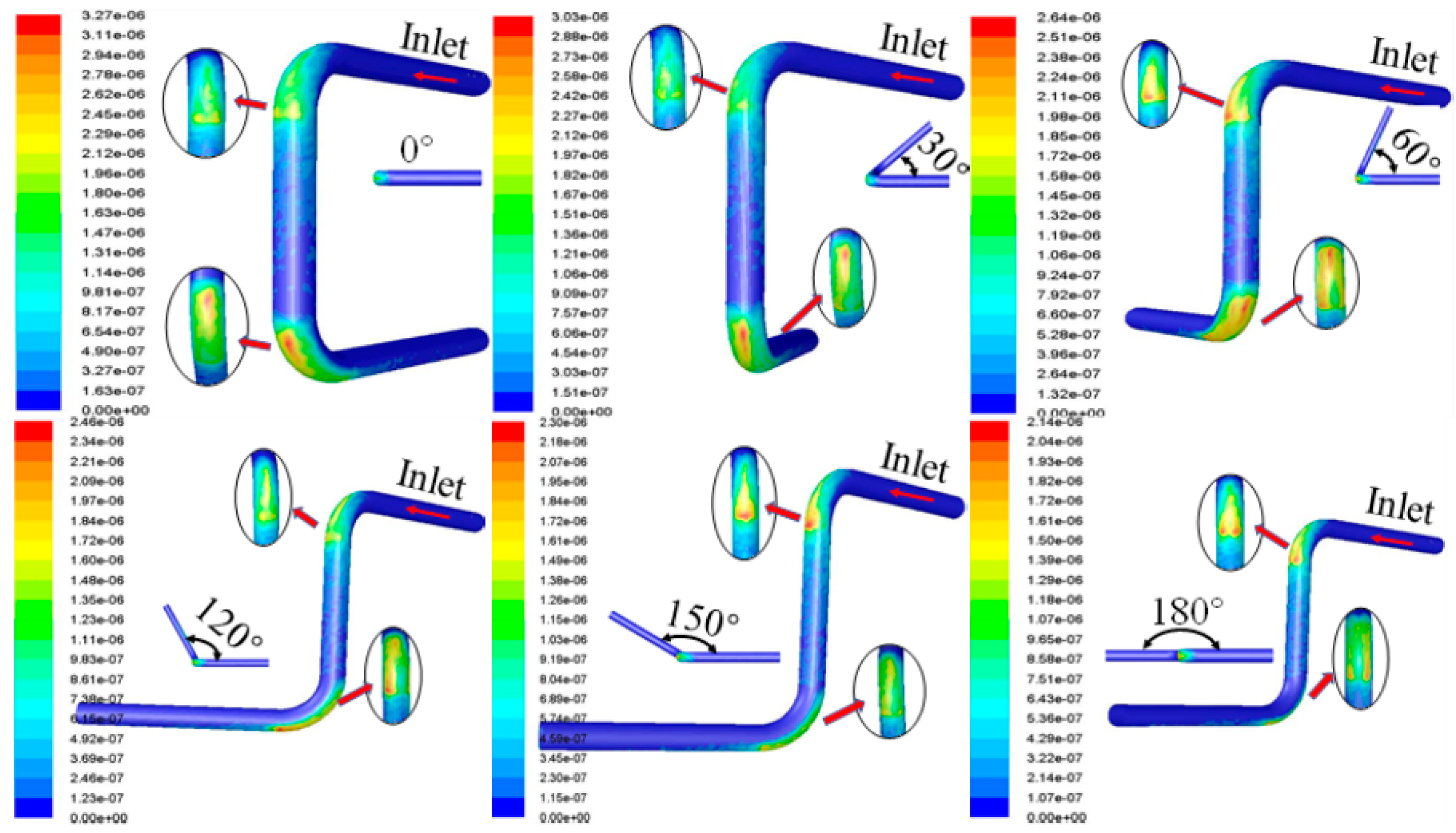
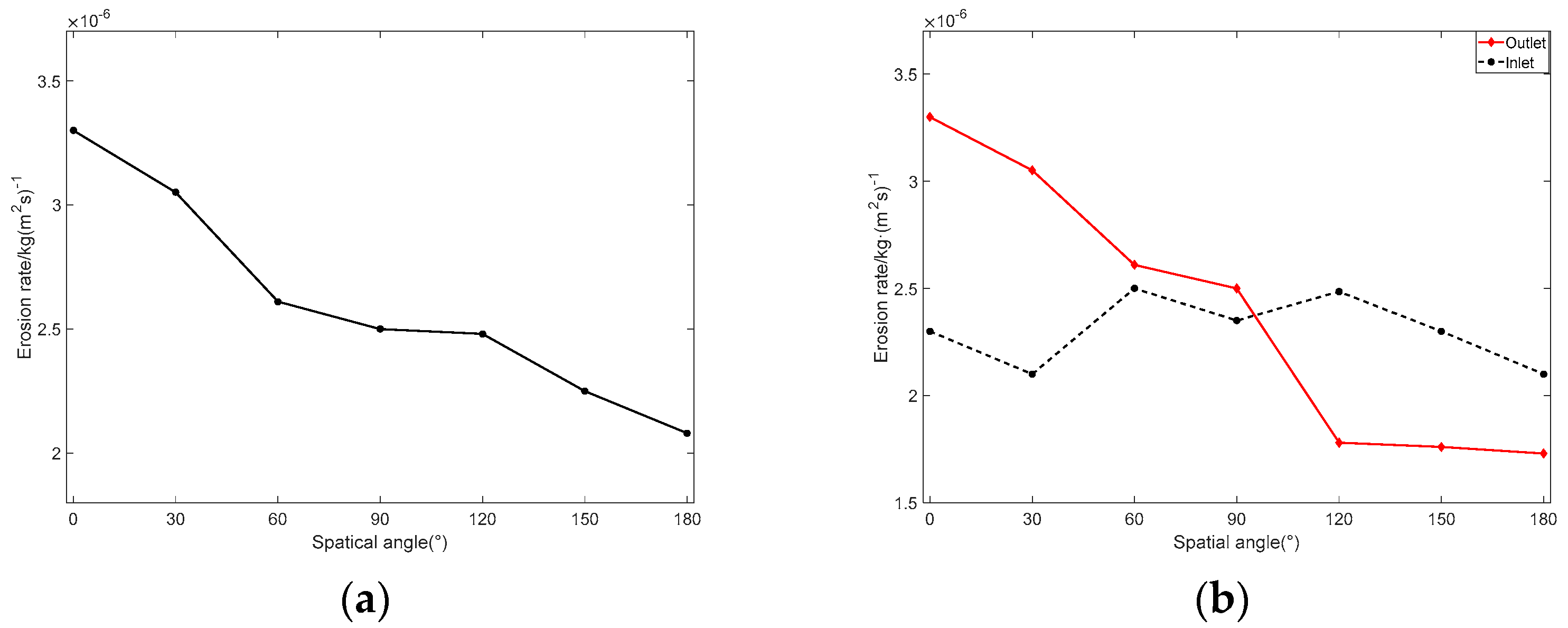
4.3. The Impact of the Spatial Angle on Pipe Elbow Erosion Wear

The pipeline structure of the connected section of the two bends can be rotated relative to each other. Changing the space angle between the two bends, the liquid phase fluid flows through the two sections of the bend [24]. The flow direction is different, resulting in different rates of erosion and wear. A cloud diagram of different angles of pipeline structure erosion wear is shown in Figure 15.

An increase in the spatial angle of the two sections of the bend is shown in Figure 15. The maximum erosion location of the bend is changed from the lower end near the outlet end of the bend to the upper end near the inlet end of the bend. However, the maximum erosion wear rate at the first section of the bend does not change greatly. This is due to the two sections of the bend at a low angle and the convex wall of the bend being in the same party. The particles flow along the outer wall of the connecting straight pipe after flowing through the first section of the bend. When the spatial angle is greater than 30°, the maximum erosion area of the lower bend is deflected to the side of the bend. In addition, there are multiple erosion peaks. When the connection angle exceeds 90°, only a small portion of the particles flowing downstream along the wall of the straight pipe will accumulate at the second section of the bend [25]. This reduces the second bend erosion wear rate.

As illustrated in Figure 16a, the maximum erosion wear rate decreases as the spatial angle between the two bends increases. Between 90° and 120°, the maximum erosion rate changes less as the spatial angle between the two bends increases. As shown in Figure 16b, the maximum erosion wear rate at the inlet end of the bend floats up and down around a certain value as the spatial clamp angle increases, but the difference is small. Meanwhile, the maximum erosion wear rate at the exit end of the bend gradually decreases with the increase in the spatial angle [26]. When the spatial angle exceeds 120°, the erosion wear rate tends to stabilize.

5. Analysis of the Erosion Resistance of Different Designs of Elbow Pipe Types

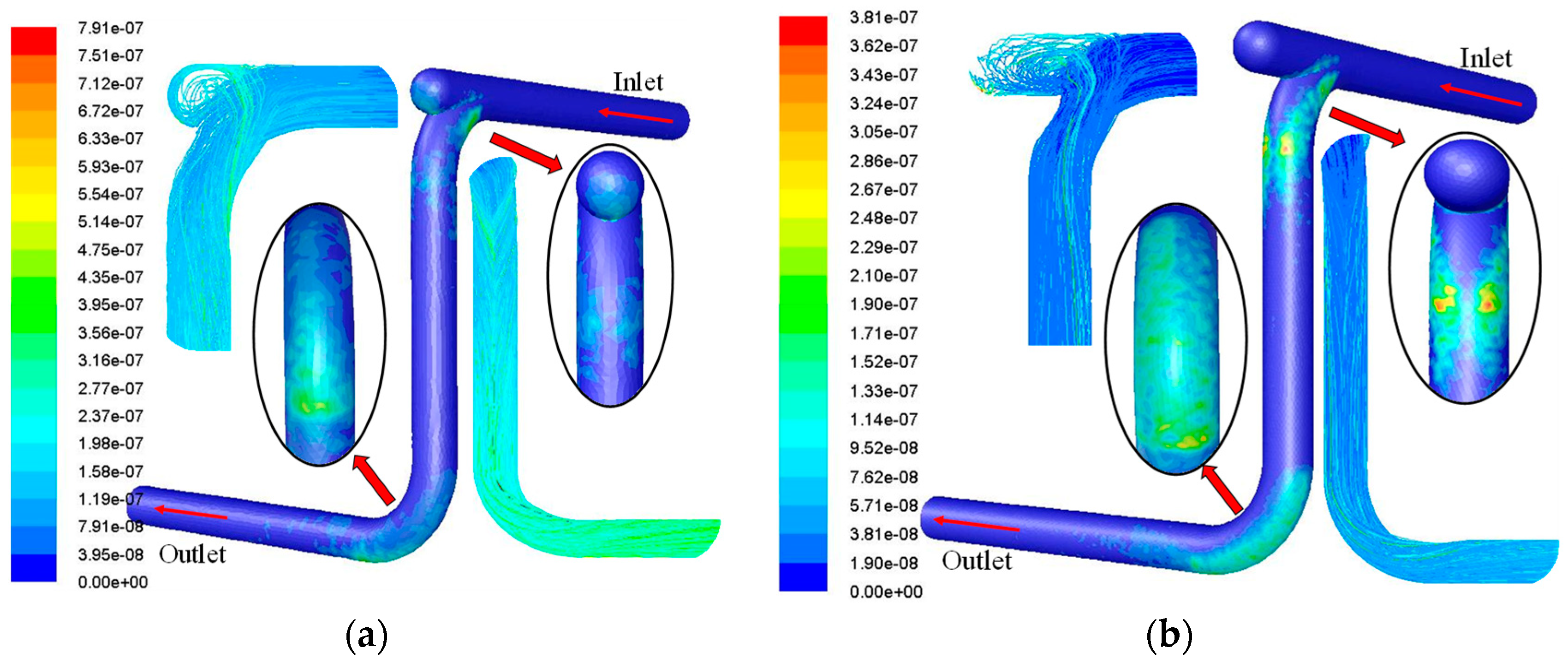
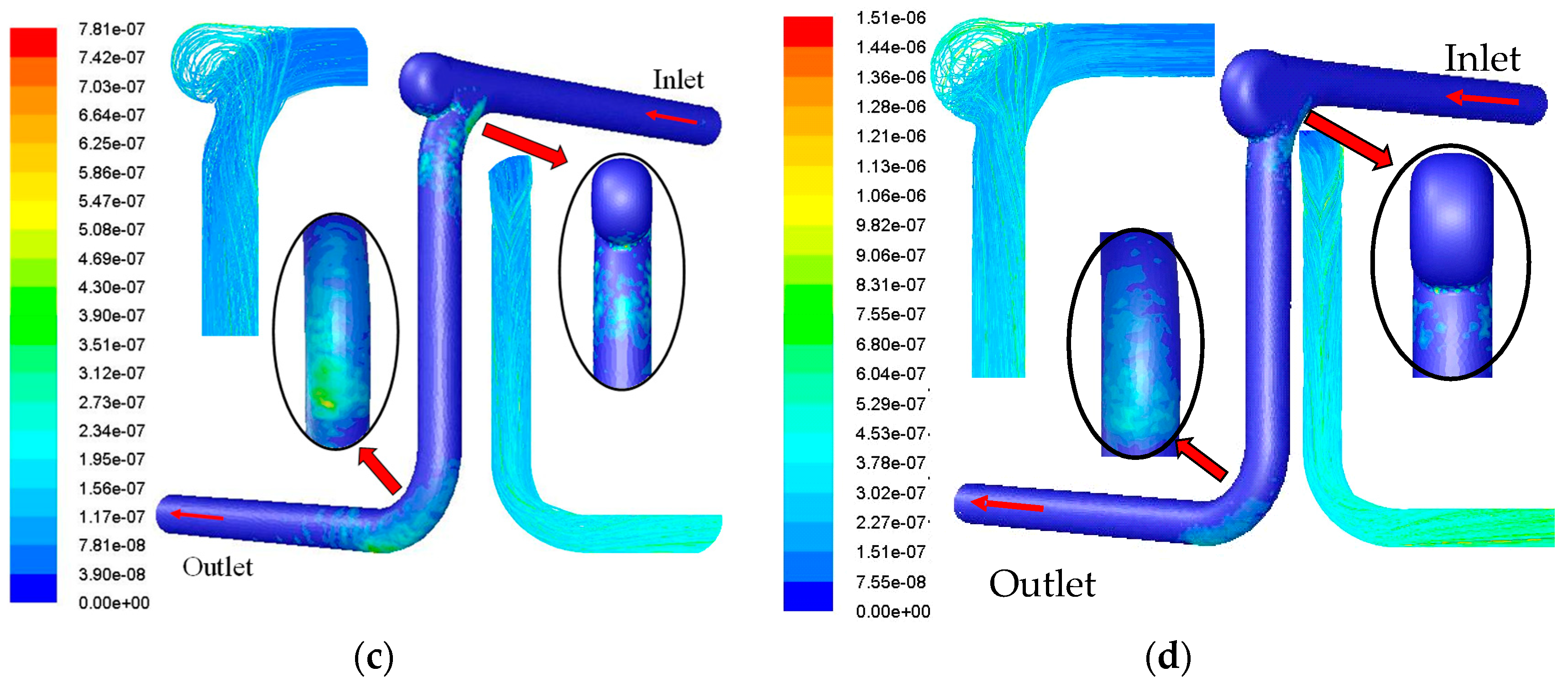
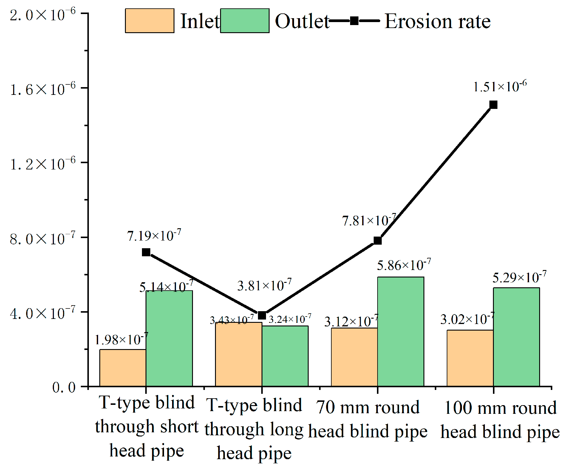
5.1. Optimization of the Erosion Resistance of Blind Bends

(1)

Geometric model

In this section, without changing the overall dimensions of the space pipeline structure, a section of the blind pass pipe structure commonly used in engineering is added at the inlet end bend. Different blind pipes are added through the structure, as shown in the Figure 17, Figure 18, Figure 19 and Figure 20. All the model pipe diameters are D = 50 mm, the inlet and outlet end lengths are 8D = 400 mm, the bend radius at the elbow is R = 2D = 100 mm and the intermediate straight section is 6D = 300 mm.

(2)

Initial boundary conditions and meshing

In the boundary condition setting, the inlet end is set to velocity inlet, the discrete phase of the inlet and outlet ends is set to escape and the wall condition is set to the default no-slip boundary. The discrete phase of the pipe wall is set as reflect, the gravitational acceleration is 9.8 m/s², the mass flow rate of the particles is 0.2 kg/s, the particle diameter is 0.00045 m and the impact angle function of the particles is defined in a segmented linear way.

There is a certain amount of energy dissipation after the sand particles collide with the inner wall of the pipeline. This results in the particle velocity after collision being less than the initial velocity at the time of incidence. The energy dissipation before and after sand particle impact is defined using the wall recovery coefficient [27,28,29].

(3)

Numerical simulation results and analysis

The numerical simulation method is used to calculate and analyse four common blind pass pipe types with different lengths and sizes using Fluent software. The erosion and wear results and the particle trajectories obtained are shown in Figure 16.

As revealed in Figure 21, the number of particles entering the blind pass increases as the length and area of the T-shaped blind pass tube increases. The residence time of particles in the blind pass increases. The erosion wear rate at the pipe elbows as well as the maximum erosion wear rate decreases significantly, and the area of erosion wear is more uniform. The location of maximum erosion for a typical pipeline structure is at the lower end of the bend. In contrast, the maximum erosion location of the blind pass tube is at the junction of the blind pass tube and the elbow [30]. From the particle trajectories, it can be seen that when the particles re-enter the region of the bent tube, they cause impact wear on the concave wall surface of the bent tube. The erosion wear of the elbow by particles in the liquid phase is no longer limited to the convex wall of the elbow near the outlet straight end. The smaller maximum erosion rate and the dispersion of the erosion peaks in several places prolong the life of the bend. This also increases the utilization of the bend.

As can be seen in Figure 22, among the four types of blind pass tubes, the T-type short head elbow is located in the region of the least erosion wear, whereas the T-type blind pass long pipe is the most effective in suppressing erosion wear at the second section of the elbow. The T-type blind pass long header pipe has the smallest maximum rate of erosion wear.

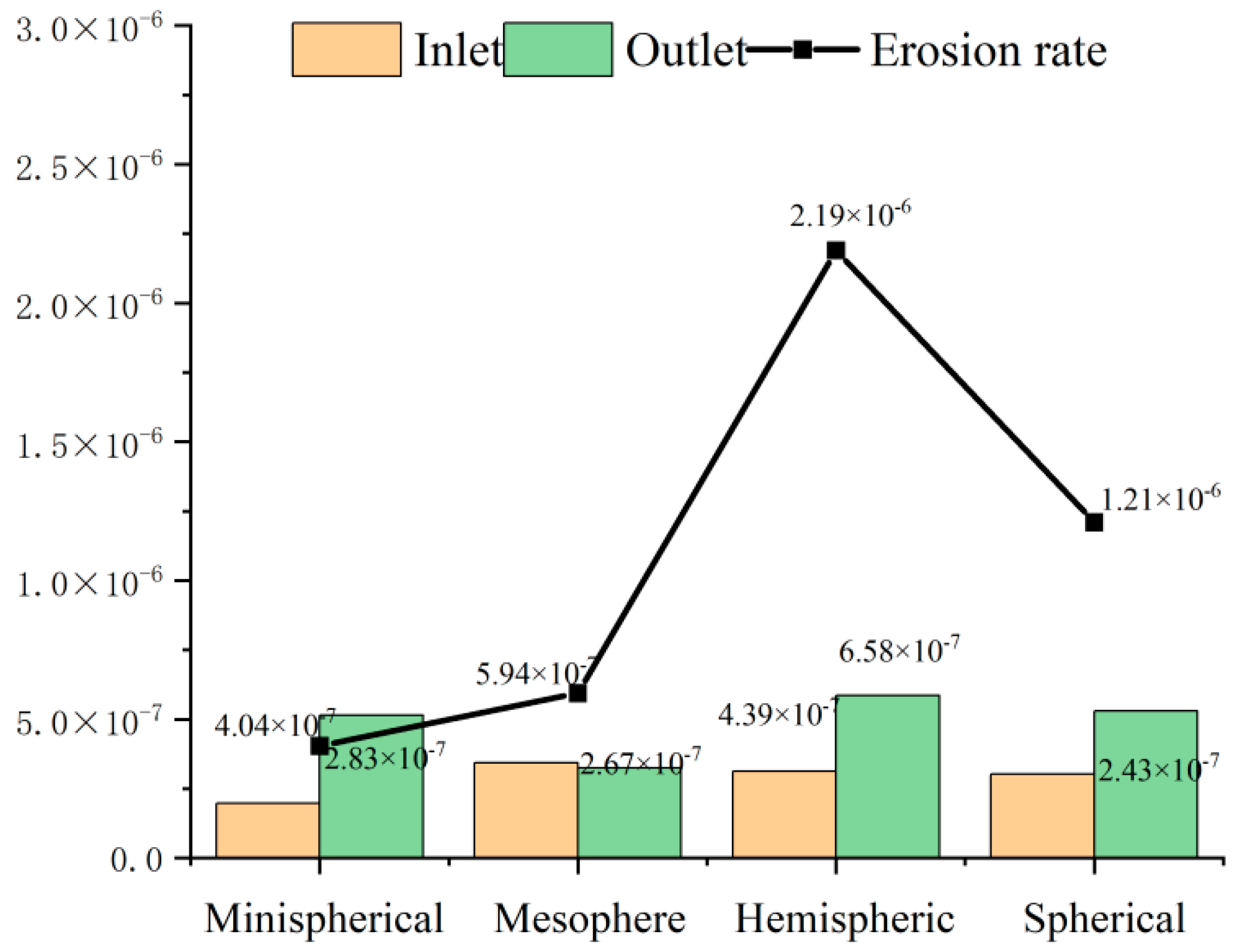
5.2. Optimization of the Erosion Resistance of a Spherical Bend

(1)

Geometric model

We examined the influence of pipe diameter on the erosion and wear of the bend. With other conditions remaining unchanged, we gradually expanded the pipe diameter at the inlet end of the bend. Four types of bend structures were formed: small ball type, medium ball type, hemispherical type and spherical type, as shown in Figure 23. All the model pipe diameters are $D=50$ mm, the lengths of the inlet and outlet ends are $L1=L3=400$ mm, the bending radii at the bends are $R1=R2=2D=100$ mm and the intermediate straight sections are $L2=300$ mm.

(2)

Numerical simulation calculation results and analysis

As shown in Figure 24, the particle beams of the four tube types disperse in all directions after hitting the spherical wall. The particles eventually converge along the wall of the bent tube at the concave wall of the bent tube and then flow with the liquid phase again. After entering the second section of the straight pipe, the particles flow uniformly along the wall of the straight pipe. In contrast, the particle bundles of a typical pipeline structure are concentrated at the convex wall of the first bend to enter the straight tube and flow along the side of the straight pipe. The bent pipe, after changing the bent pipe structure, improves the utilization of the whole pipe.

The small ball pipe bend and the medium ball pipe bend have a curved surface connection with the straight pipe. The maximum erosion location is in the transition area between the two sides of the bend and the straight pipe connection, instead of the concave wall surface and the straight pipe connection. In the hemispherical bends and spherical bends, the maximum erosion location is in the spherical bend and the straight pipe connection of the mutation. The erosion area is in the form of a band [31]. The erosion wear area at the second section of the second bend of the four pipe structures is widely and uniformly distributed, and the erosion rate is small. The location of the erosion peak is similar to the erosion location of a typical pipeline structure.

Figure 25 displays that the maximum erosion rate of the small ball type is the smallest. The bend at the change in pipe shape has the least erosion wear. Meanwhile, the hemispherical-type bend has the most severe erosion wear at the second section of the bend, and the erosion rate is larger.

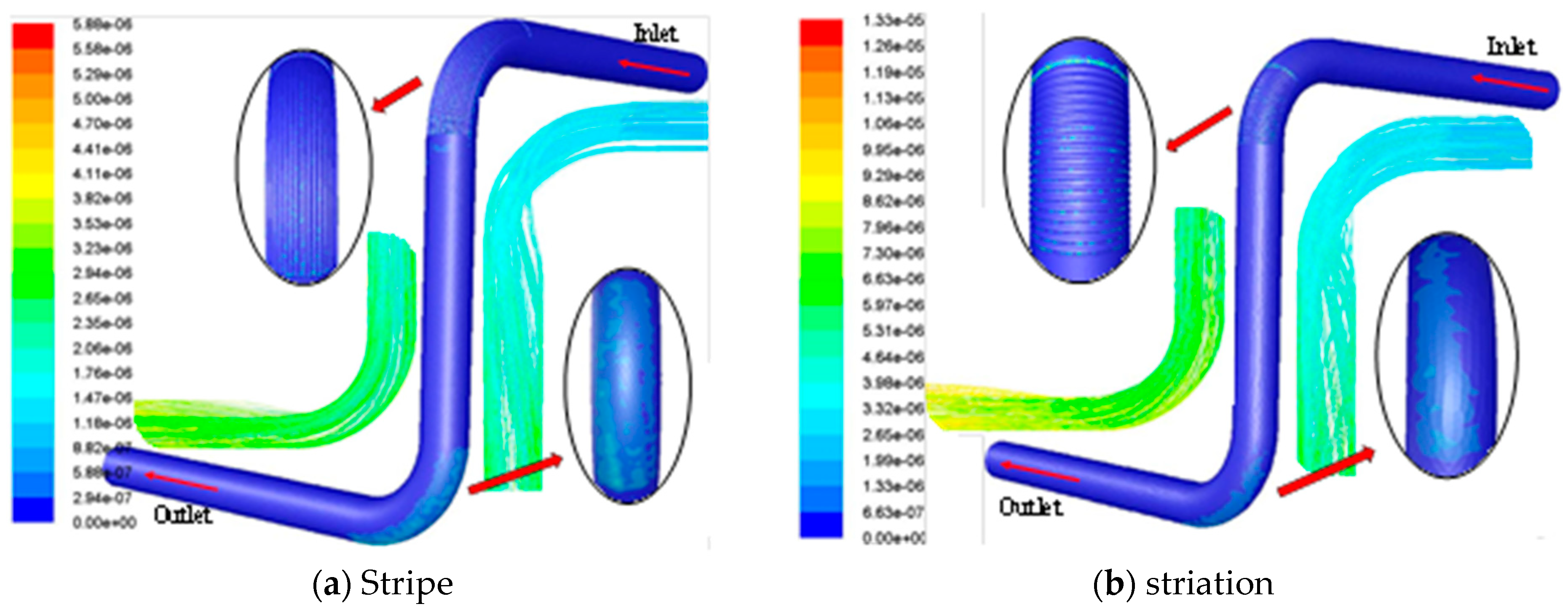
5.3. Scour Analysis of the Inner Wall Surface of Corrugated Bends

(1)

Geometrical model

This analysis was conducted according to the wear-resistant morphology of the shell of shellfish organisms. We established transverse corrugated and longitudinal corrugated types of bionic inner wall thickening bent pipe models, as illustrated in Figure 26. The models are different except for the morphology of the inner wall surface at the bend. The shape and size of the rest of the area are the same as those of a typical pipeline structure.

(2)

Numerical simulation results and analysis

The particle beam in Figure 27a is split by longitudinal ripples at the near-wall surface. The particle beam in Figure 27b is clearly blocked by the transverse ripples at the near-wall surface, and some of the particle trajectories are changed. The change in particle trajectory at the second bend is not obvious. The erosion rate at the longitudinal corrugated bend is distributed in the groove pits in a point-like manner. The maximum erosion rate is located at the stripe protrusion at the inlet end of the bend, and the peak of erosion at the bend near the outlet end of the pipe is significantly increased. The maximum erosion at the transverse corrugated bend is located at the beginning of the transverse corrugated end face of the bend in a band-like distribution, the entire transverse corrugated wall appears in a number of erosion peaks and the distribution is scattered. However, the erosion peaks of the two bellows are mostly distributed in a point-like manner, and the erosion area is small. Most of the area of the bend has a lower erosion rate, which makes the bend more wear-resistant. The erosion region at the second section of the bend in the two structures is similar to that in a typical pipeline structure.

As can be seen from Figure 28, the maximum erosion rate of the longitudinal corrugated pipeline structure is smaller. The erosion rate at the second section of the bend is smaller than that of the transverse corrugated bend.

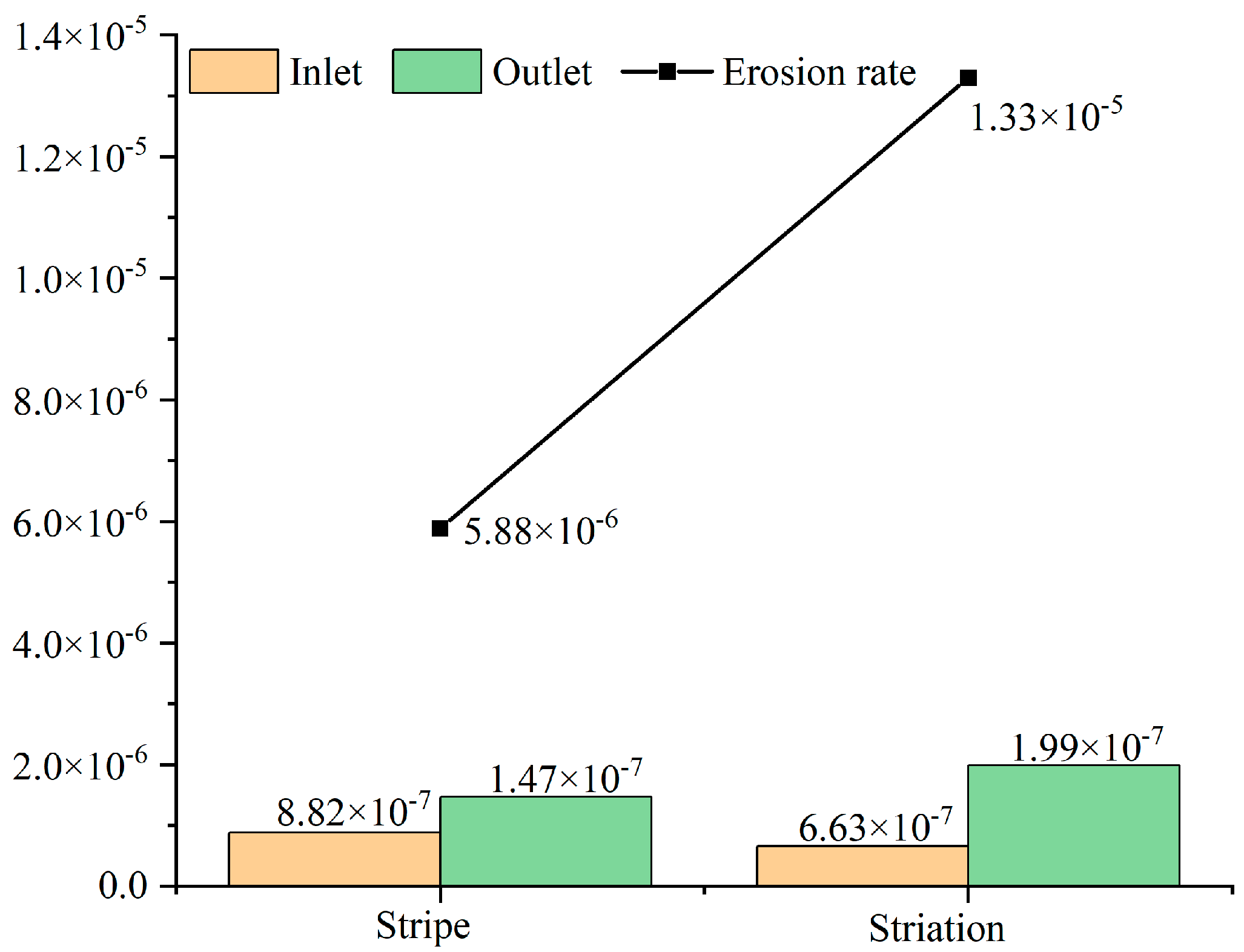
5.4. Comparative Analysis of Results

Here, we present a comparative analysis of the abovementioned 10 pipeline structure types and the typical pipeline structure from the previous paper, with the aggregated results shown in

Table 5. Erosion rate.

Pipeline Type	Upper End Elbow Erosion Rate kg/(m2·s)	Lower End Elbow Erosion Rate kg/(m2·s)	Maximum Erosion Rate kg/(m2·s)	Reduction from Original Structure
Typical pipeline structure	$2.34\times {10}^{-6}$	$2.47\times {10}^{-6}$	$2.47e\times {10}^{-6}$	——
T-type blind through short header pipe	$1.98\times {10}^{-7}$	$5.14\times {10}^{-7}$	$7.19\times {10}^{-7}$	70.89%
T-type blind through long header pipe	$3.43\times {10}^{-7}$	$3.24\times {10}^{-7}$	$3.81\times {10}^{-7}$	84.57%
70 mm round head blind pipe	$3.12\times {10}^{-7}$	$5.86\times {10}^{-7}$	$7.81\times {10}^{-7}$	68.38%
100 mm round head blind pipe	$3.02\times {10}^{-7}$	$5.29\times {10}^{-7}$	$1.15\times {10}^{-6}$	53.44%
Minispherical	$4.04\times {10}^{-7}$	$2.83\times {10}^{-7}$	$4.04\times {10}^{-7}$	83.64%
Mesopherical	$5.94\times {10}^{-7}$	$2.67\times {10}^{-7}$	$5.94\times {10}^{-7}$	75.95%
Hemispherical	$4.39\times {10}^{-7}$	$6.58\times {10}^{-7}$	$2.19\times {10}^{-6}$	11.34%
Spherical	$1.21\times {10}^{-6}$	$2.43\times {10}^{-7}$	$1.21\times {10}^{-6}$	51.01%
Stripe	$8.82\times {10}^{-7}$	$1.47\times {10}^{-6}$	$5.88\times {10}^{-6}$	−138.06%
Striation	$6.63\times {10}^{-7}$	$1.99\times {10}^{-6}$	$1.33\times {10}^{-5}$	−438.46%

. The structure with the smallest maximum erosion rate is the T-type blind pass long header pipe. The minimum erosion rate at the upper-end elbow is found in the T-type blind pass stubby pipe. The ball-type elbow has the lowest erosion rate at the lower end elbow. With the above analysis, it was found that each type of elbow has its own erosion-resistance characteristics. The value of the erosion rate can be seen from the size of the T-type blind through the elbow pipe with the more obvious anti-erosion effect. However, from the previous erosion cloud diagram, it can be seen that the bionic corrugated bends have better erosion resistance.

6. Conclusions

The erosion and wear patterns of pipeline elbows under different structural parameters were analysed in this study. The following conclusions were obtained:

(1)

The degree of influence of each structural parameter on the erosion wear in descending order is as follows: bending angle, bending diameter ratio and spatial angle.

(2)

With the increase in the bending diameter ratio, the erosion wear rate of the pipeline structure gradually decreases. With the increase in the bending angle of the elbow, the maximum erosion rate of the pipeline elbow changes less before 90° and gradually increases beyond 90°. When the space clamping angle increases, the maximum erosion rate of the pipeline structure gradually decreases.

(3)

The bend to increase the blind tube can effectively reduce the erosion rate and slow down the erosion effect. An appropriate increase in the length and volume of the blind pass tube can also reduce erosion wear at the bend. Spherical bends make the particle distribution more uniform. The spherical diameter of the smaller bend has a greater anti-erosion effect than the larger diameter of the spherical bends. The maximum erosion rate of the corrugated pipe is higher than that of other structures, but its low erosion rate distribution area is wider, and the peak is more distributed in point form.

(4)

A new structure based on the bionic structure for optimizing the erosion resistance of pipe elbows is proposed. The influence of different structure sizes and other factors at the bends in resisting erosion is studied comparatively. It is then verified that the corrugated structure has a better erosion-resistance effect. This provides a reference for the further design and optimization of the pipeline.

(5)

As a result of the oil and gas extraction process, multiple factors working together have an impact on bend erosion wear. The method of controlling a single variable used in this study has caused the erosion wear numerical simulation results to deviate from the experimental, and even actual, working conditions. In subsequent studies, more situations will be considered to ensure that the numerical simulation results are more accurate. In this paper, a new optimization structure of bending pipes based on a bionic structure is proposed that has good application prospects, but more attention needs to be paid to its preparation.

References

1. Mills, D.; Mason, J.S. Particle size effects in bend erosion. Wear 1977, 44, 311–328. [Google Scholar] [CrossRef]
2. Kosinska, A.; Balakin, B.V.; Kosinski, P. Theoretical analysis of erosion in elbows due to flows with nano- and micro-size particles. Powder Technol. 2020, 364, 484–493. [Google Scholar] [CrossRef]
3. Throneberry, J.M.; Zhang, Y.; McLaury, B.S. Solid-Particle erosion in slug flow. In Proceedings of the SPE Annual Technical Conference and Exhibition, Florence, Italy, 20–22 September 2010. [Google Scholar]
4. Kesana, N.R.; Throneberry, J.M.; Mc Laury, B.S.; Shirazi, S.A.; Rybicki, E.F. Effect of particle size and liquid viscosity on erosion in annular and slug flow. Energy Resour. Technol. 2013, 136, 012901. [Google Scholar] [CrossRef]
5. Chen, X.; Mclaury, B.S.; Shirazi, S.A. Application and experimental validation of a computational fluid dynamics (CFD)-based erosion prediction model in elbows and plugged tees. Comput. Fluids 2004, 33, 1251–1272. [Google Scholar] [CrossRef]
6. Grant, G.; Tabakoff, W. Erosion prediction in turbomachinery resulting from environmental solid particles. J. Aircr. 1975, 12, 471–478. [Google Scholar] [CrossRef]
7. Mazumder, Q.H.; Shirazi, S.A.; McLaury, B. Experimental Investigation of the location of maximum erosive wear damage in elbows. J. Press. Technol. 2008, 130, 244–254. [Google Scholar] [CrossRef]
8. Pereira, G.C.; Jos, S.F.; Alves, M.M.D. Numerical prediction of the erosion due to particles in elbows. Powder Technol. 2014, 261, 105–117. [Google Scholar] [CrossRef]
9. Wood, R.; Jones, T.F.; Miles, N.J. Upstream swirl-induction for reduction of erosion damage from slurries in pipeline bends. Wear 2001, 250, 770–778. [Google Scholar] [CrossRef]
10. Hashish, M. An improved model of erosion by solid particle impact. In Proceedings of the Erosion by Liquid and Solid Impact, Seventh International Conference, Cambridge, UK, 7 September 1987; p. 66. [Google Scholar]
11. Solnordal, C.B.; Wong, C.Y.; Boulanger, J. An experimental and numerical analysis of erosion caused by sand pneumatically conveyed through a standard pipe elbow. Wear 2015, 336–337, 43–57. [Google Scholar] [CrossRef]
12. Wood, R.J.K.; Jones, T.F.; Ganeshalingam, J. Comparison of predicted and experimental erosion estimates in slurry ducts. Wear 2004, 256, 937–947. [Google Scholar] [CrossRef]
13. Zahedi, P.; Zhang, J.; Arabnejad, H. CFD simulation of multiphase flows and erosion predictions under annular flow and low liquid loading conditions. Wear 2017, 376–377, 1260–1270. [Google Scholar] [CrossRef]
14. Zhang, Y.; Reuterfors, E.P.; McLaury, B.S. Comparison of computed and measured particle velocities and erosion in water and air flows. Wear 2007, 263, 330–338. [Google Scholar] [CrossRef]
15. Zhang, J.; Darihaki, F.; Shirazi, S.A. A comprehensive CFD-based erosion prediction for sharp bend geometry with examination of grid effect. Wear 2019, 430–431, 191–201. [Google Scholar] [CrossRef]
16. Peng, W.; Cao, X. Numerical simulation of solid particle erosion in pipe bends for liquid–solid flow. Powder Technol. 2016, 294, 266–279. [Google Scholar] [CrossRef]
17. Jianlin, S.Z.; Zhang, Z.-y.; Tong, H.; Yan, S.; Peixin, G.; Tao, Y. Analysis of Erosion Characteristics of Liquid-solid Two-phase Fiow in Space Z-shape Pipeline. Chin. Hydraul. Pneum. 2022, 46, 34–43. (In Chinese) [Google Scholar]
18. Zhang, Q.; Rahmatjan, I.; Memetimin, G. Design of flow characteristics and optimization of guided pneumatic. Chin. Hydraul. Pneum. 2021, 45, 44–51. (In Chinese) [Google Scholar]
19. Ren, J.; Wang, J.; Min, W. Analysis of influence of valve port sealing width on flow field characteristics of piezoelectric pneumatic microvalve with nozzle baffle. Chin. Hydraul. Pneum. 2021, 45, 58–67. (In Chinese) [Google Scholar]
20. Vivek, K. FLUENT 6.3 User’s Guide; Fluent Inc.: Lebanon, PA, USA, 2006. [Google Scholar]
21. Yakhot, V.; Orszag, S.A. Renormalization group analysis of turbulence. I. Basic theory. J. Sci. Comput. 1986, 1, 3–51. [Google Scholar] [CrossRef]
22. Morsi, S.A.; Alexander, A.J. An investigation of particle trajectories in two-phase flow systems. J. Fluid Mech. 1972, 55, 193–208. [Google Scholar] [CrossRef]
23. Banakermani, M.; Naderan, H.; Saffar-Avval, M.J.P.T. An investigation of erosion prediction for 15 to 90 elbows by numerical simulation of gas-solid flow. Powder Technol. 2018, 334, 9–26. [Google Scholar] [CrossRef]
24. Ghosh, A. Validated Numerical Simulations Investigating the Effects of Cross-sectional Asymmetry on Fluid Flow and Heat Transfer. Ph.D. Thesis, University of Minnesota, Minneapolis, MN, USA, 2017. [Google Scholar]
25. Yan, Y.; Zhao, Y.; Yao, J.; Wang, C.-H.J.P.T. Investigation of particle transport by a turbulent flow through a 90° bend pipe with electrostatic effects. Powder Technol. 2021, 394, 547–561. [Google Scholar] [CrossRef]
26. Cao, L.; Tu, C.; Hu, P.; Liu, S.J.A.T.E. Influence of solid particle erosion (SPE) on safety and economy of steam turbines. Appl. Therm. Eng. 2019, 150, 552–563. [Google Scholar] [CrossRef]
27. Zolfagharnasab, M.; Salimi, M.; Zolfagharnasab, H.; Alimoradi, H.; Shams, M.; Aghanajafi, C.J.P.T. A novel numerical investigation of erosion wear over various 90-degree elbow duct sections. Powder Technol. 2021, 380, 1–17. [Google Scholar] [CrossRef]
28. Panda, K.; Hirokawa, T.; Huang, L.J.A.T.E. Design study of microchannel heat exchanger headers using experimentally validated multiphase flow CFD simulation. Appl. Therm. Eng. 2020, 178, 115585. [Google Scholar] [CrossRef]
29. Zonglin, S.; Zhenhua, X.; Mengyun, Z.; Pengfei, D.; Yuguo, W. Numerical simulation research in erosion-corrosion of 90 elbow pipe. J. Liaoning Univ. Pet. Chem. Technol. 2018, 38, 47. [Google Scholar]
30. Han, F.; Ong, M.C.; Xing, Y.; Li, W.J.O.E. Three-dimensional numerical investigation of laminar flow in blind-tee pipes. Ocean. Eng. 2020, 217, 107962. [Google Scholar] [CrossRef]
31. Wang, F.; Sahana, M.; Pahlevanzadeh, B.; Pal, S.C.; Shit, P.K.; Piran, M.J.; Janizadeh, S.; Band, S.S.; Mosavi, A. Applying different resampling strategies in machine learning models to predict head-cut gully erosion susceptibility. Alex. Eng. J. 2021, 60, 5813–5829. [Google Scholar] [CrossRef]
Figure 1. Schematic diagram of the model.
Applsci 14 00984 g001
Figure 2. Mesh division.
Applsci 14 00984 g002
Figure 3. Plot of the erosion rate of 90° bends.
Applsci 14 00984 g003
Figure 4. Experimental diagram of erosion and wear.
Applsci 14 00984 g004
Figure 5. Speed vector cloud diagram.
Applsci 14 00984 g005
Figure 6. Pressure cloud diagram.
Applsci 14 00984 g006
Figure 7. Cloud diagram of the particle trajectory.
Applsci 14 00984 g007
Figure 8. Erosion cloud map.
Applsci 14 00984 g008
Figure 9. Angle view of elbow.
Applsci 14 00984 g009
Figure 10. Cloud diagram showing the effect of the bending diameter ratio on erosion wear. (a) Erosion cloud after changing the bending diameter ratio of the inlet end elbow. (b) Erosion cloud after changing the bending diameter ratio of the outlet end elbow.
Applsci 14 00984 g010
Figure 11. Effect of the bending diameter ratio on the erosion wear of the bends. (a) Comparison of the maximum erosion rate of the two-spatial pipeline structure. (b) Changing the bending diameter ratio of the inlet end elbow. (c) Changing the bending diameter ratio of the outlet end elbow.
Applsci 14 00984 g011
Figure 12. The effect of changing the bending angle at the inlet end on the erosion wear of pipe elbows.
Applsci 14 00984 g012
Figure 13. The effect of changing the bending angle at the outlet end on the erosion wear of pipe elbows.
Applsci 14 00984 g013
Figure 14. Effect of the bending angle on erosion wear. (a) Comparison of the maximum erosion rate of a two-pipeline structure. (b) Changing the bending angle of the inlet end elbow. (c) Changing the bending angle of the outlet end elbow.
Applsci 14 00984 g014
Figure 15. The effect of changing the spatial angle on the erosion wear of space pipe elbows.
Applsci 14 00984 g015
Figure 16. Relationship between the spatial angle and the erosion rate. (a) Relationship between the erosion rate and angle. (b) Changes in pipe erosion rate of bends.
Applsci 14 00984 g016
Figure 17. T-type blind through short header pipe.
Applsci 14 00984 g017
Figure 18. T-type blind through long header pipe.
Applsci 14 00984 g018
Figure 19. Round head blind pipe measuring 70 mm.
Applsci 14 00984 g019
Figure 20. Round head blind pipe measuring 100 mm.
Applsci 14 00984 g020
Figure 21. Particle trajectory diagrams for different blind pipe structures: (a) T-type blind through short header pipe; (b) T-type blind through long header pipe; (c) 70 mm round head blind pipe; and (d) 100 mm round head blind pipe.
Applsci 14 00984 g021aApplsci 14 00984 g021b
Figure 22. Comparison of erosion rates for different blind tubes.
Applsci 14 00984 g022
Figure 23. Space pipeline structure with different bend structures.
Applsci 14 00984 g023
Figure 24. Particle trajectories for different bends.
Applsci 14 00984 g024aApplsci 14 00984 g024b
Figure 25. Comparison of erosion rates for different bends.
Applsci 14 00984 g025
Figure 26. Two pipeline structures.
Applsci 14 00984 g026
Figure 27. Particle trajectories for different pipeline structures.
Applsci 14 00984 g027
Figure 28. Comparison of erosion rates for two pipelines.
Applsci 14 00984 g028