Article

Dependence of Sensitivity Factors on Ratio of Traffic Load to Dead Load

Faculty of Civil Engineering, University of Belgrade, 11120 Belgrade, Serbia
*
Author to whom correspondence should be addressed.
Appl. Sci. 2024, 14(3), 985; https://doi.org/10.3390/app14030985
Submission received: 29 December 2023 / Revised: 19 January 2024 / Accepted: 20 January 2024 / Published: 24 January 2024
(This article belongs to the Special Issue Infrastructure Management and Maintenance: Methods and Applications)

Abstract

:
According to modern structural codes, a design is considered to be adequate if the limit states are not exceeded. For the ultimate limit state, the design value of action effect Ed is required to be less or equal than the design value of ultimate resistance Rd. This ensures, according to the Eurocode, a sufficiently low probability of failure expressed as the target reliability index β. Consequently, the distributions of action effect and of resistance need to satisfy the following conditions: P E > E d Φ + α E β and P R R d Φ α R β , where αE and αR, with |α| ≤ 1, are the values of the FORM sensitivity factors. The values of the sensitivity factors αE and αR are suggested, according to EN1990, as −0.7 and 0.8, respectively; for the accompanying actions, the sensitivity factor is recommended as 0.28. In this paper, the dependence of the sensitivity factors for traffic live load, dead load, and resistance on the ratio of traffic load to dead load is studied (which is directly proportional to the maximum span of the bridge). Significantly different sensitivity factors for resistance, dead load, and traffic load, other than proposed by the Eurocode, has been calculated for typical ratio of traffic to dead load. It further showed that, if it is assumed that Ed = Rd and the Eurocode partial safety factors are used, a different design point than the starting point, i.e., Ed = Rd, is obtained.

1. Introduction

According to the modern structural codes such as the Eurocode [1] and Swiss Code [2], a design is considered to be adequate if the limit states are not exceeded. For the ultimate limit state, the design value of action effect Ed is required to be less than or equal to the design value of ultimate resistance Rd. This ensures, according to the Eurocode, sufficiently low probability of failure expressed as the reliability index β. In order to check whether this requirement holds, one needs to obtain distribution of both action effect and resistance. Using one of the reliability methods, e.g., FORM (First Order Reliability Method, the most common technique of structural reliability analysis) one can evaluate the reliability index β, most likely the failure point and also sensitivity factors α E and α R . Consequently, the distributions of action effect and of resistance need to satisfy the following conditions P E > E d Φ + α E β and P R R d Φ ( α R β ) where αE and αR, with |α| ≤ 1, are the values of the FORM sensitivity factors.
In this paper, the dependence of the sensitivity factors for traffic live load, dead load, and resistance on the ratio of traffic load to dead load is studied. Further, the ratio of traffic load to dead load effects is proportional to the maximum span of the bridge. Changing the sensitivity factors, and keeping the same probability distribution for random variables, indicates the most likely failure points are changing. Equalizing the most likely failure point with the design value of the action affect and ultimate resistance, one can obtain partial factors. Taking into account the dependence of the sensitivity factor on the ratio between traffic load and dead load, the correct partial factors for new or existing bridges can be calibrated in defining the load models and satisfying the target safety index (and consequently, the probability of failure).
Sensitivity factors may be interpreted as factors giving the relative importance of the individual random variable for the reliability index β, i.e., the probability of failure, as shown graphically in Figure 1. The sensitivity factors αE and αR may be taken according to EN1990 as −0.7 and 0.8, respectively. For the accompanying actions, the design values may be defined by P(E > Ed) = Φ(−0.4 × 0.7 × β) = Φ(−0.28β). The condition for these expressions are that 0.16 < σ E / σ R < 7.16 , where σ E and σ R are standard deviations for the action effect and for resistance, respectively. Otherwise, α = ±1.0 should be used for the variable with the larger standard deviation, and α = ±0.4 for the variable with the smaller standard deviation. These values of the sensitivity factors are based on the study where the deviation from the target reliability index for different values of the ratio between the standard deviation of the random variable R and E was minimized [3].
The fib Bulletin 80 [4] proposes two methodologies devoted to the redefinition of the partial safety factors for the assessment of existing structures: the design value method (DVM) and the adjusted partial factor method (APFM). The DVM allows for recalculation of the partial safety factors for both resistances and actions by means of consistent probabilistic models derived by the prior knowledge, test results, and observations related to the existing structure under investigation. The APFM, which can be considered the simpler approach, allows for the update of the partial safety factors defined by the Eurocode for new structures by means of “adjustment coefficients” accounting for the prior knowledge, test results, and observations related to the existing structure. However, in both of these methods, the FORM sensitivity factors αR and αE, which are direct parameters used in calculation, are set equal to 0.8 and −0.7 for dominant variables, respectively, and are equal to 0.32 and −0.28 for nondominant variables. A resistance variable is considered dominant if its sensitivity factor calculated as α X i = C O V X i / j C O V X j 2 , (where COV is coefficient of variation and summation is undertaken over all basic resistance variables) exceeds that of the other resistance variables. The same procedure is performed for determining the dominant load variable. This approach, suggested by [4], has been applied, for example, in [5] for the assessment of the existing sample bridge by recalculating the partial factors. Further, a recalibration of the partial factors, with the corresponding use of sensitivity factors, is often of interest, for example, for the reassessment of the traffic load model [6] or for the assessment of railway bridge reliability [7].
The goal of this paper is to provide a guideline for the correct calculation of the sensitivity factors, and to show that correct values differ significantly from the proposed values from the Eurocode. Without having the accurate sensitivity factors, a proper partial factor calibration is not possible. Taking into account the dependence of the sensitivity factor on the ratio between traffic load and dead load, the correct partial factors for new or existing bridges can be calibrated in defining the load models, satisfying the target safety index (and consequently the probability of failure).

2. Methodology

In the parametric study performed herein, for the dependence of the sensitivity factors on the ratio of traffic load to dead load, a linear limit state function has been assumed in the following form: g = R-Q-G, where R represents the resistance of the structure, Q represents the traffic live load, and G represent dead load (self-weight of all components of the bridge, structural and nonstructural). Normal distributions have been assumed for all three random variables (R, Q, and G).
The reliability index for the considered limit state function can be calculated as:
β = μ R μ s C O V R × μ R 2 + C O V G × ν × μ s 2 + C O V Q × ( 1 ν ) × μ S 2
where μ R and μ S are the expected values for resistance and total load, respectively, and COVG, COVQ, and COVR are coefficient of variation for dead load, traffic live load, and resistance, respectively. The percentage of dead load to total load (equal to sum of dead and traffic load) is defined as ν.
At the same time, the sensitivity factor for traffic load, dead load, and resistance, respectively, can be expressed as:
α Q = C O V Q × 1 ν × μ S C O V R × μ R 2 + C O V G × ν × μ s 2 + C O V Q × ( 1 ν ) × μ S 2
α G = C O V G × ν × μ s C O V R × μ R 2 + C O V G × ν × μ s 2 + C O V Q × ( 1 ν ) × μ S 2
α R = C O V R × μ R C O V R × μ R 2 + C O V G × ν × μ s 2 + C O V Q × ( 1 ν ) × μ S 2
It is clear that the calculation of sensitivity factors strongly depends on the choice of the coefficient of variation (COV) for resistance, dead load, and traffic load. A literature review of the coefficient of variation for dead load (COVG), traffic live load (COVQ), and resistance (COVR) is performed in the next chapter.

3. Review of Coefficient of Variation for Resistance and for Loads

Typical resistance uncertainties are geometrical, material, and model uncertainties. In the following, only main material uncertainties are reviewed with regards to their variability. Regarding the load uncertainties, permanent and traffic loads are discussed to estimate its variation.

3.1. Resistance—Compressive Strength of Concrete

Reference property of concrete is the compressive strength fco of the standard test specimen tested, according to standard conditions and at a standard age of 28 days. The in situ compressive strength, fc, can be related to fco as [8]:
f c = α t , τ f c o λ                   M P a
where λ is a factor, taking into account the difference between the compressive strength of the concrete as measured in situ, and the strength according to standard tests on concrete cylinders; α(t,τ) is a deterministic function, which takes into account the concrete age at the loading time, t [days] and the duration of loading, τ [days]. The concrete compressive strength can be assumed to be lognormal distributed. As it has been found that λ varies only insignificantly, the in situ concrete compressive strength is proposed in the literature to be lognormal, distributed with a COV equal to 0.15 [9].
Dragojevic et al. [10] tested 6845 samples of concrete cubes for concrete compressive strength. The COV that was calculated for all of these samples was between 0.06 and 0.19, depending on the concrete class—the higher the class, the smaller the COV.
One of the basis for US design codes provides the value of COV for concrete compressive strength from 0.15-0.18, again depending on the concrete class [11]. The values of the coefficient of variation, based on many test results for cast “on-site” concrete test cylinders and cubes varies between 0.1 and 0.2 depending on the quality control, according to [12]. These values are appropriate for between batch variation (i.e., considering concretes from all sources). The coefficients of variation are roughly halved for within batch variation (i.e., for concrete from one source).
Although the statistical distribution of concrete compressive strength has been of interest for a long time, it often has a much smaller influence on structural strength and behavior than do reinforcement properties. This is entirely due to the conventional design philosophy of attempting to achieve ductility in the structure. Nevertheless, it is important for estimating reliability of reinforced columns and for serviceability investigations [12].

3.2. Resistance—Reinforcing Steel

A probabilistic model for the reinforcement yield strength is suggested as [8]:
fs = X1 + X2 + X3
where X1 is the normal distributed random variable representing the variation in the mean of different mills, X2 is the normal distributed zero mean random variable, which takes into account the variation between batches, and X3 is the normal distributed zero mean random variable, which takes into account the variation within a batch. The mean value of X1 has been found to exhibit a significant dependence on the diameter of the bar. Probabilistic models for X1, X2, X3 and area of the bar (A) is shown in Table 1. Anom is the nominal cross-sectional area, and µ can be taken as the nominal steel grade plus two standard deviations of X1. Taking into account the coefficient of variation of the bar cross-section area leads to a COV for reinforcement yield strength equal to 0.057 [8,9].
Ellingwood et al. [11] provide the COV for reinforcement yield strength equal to 0.098–0.116, while Mirza et al. suggest that COV for reinforcement yield strength is likely to be around 4–7% [13].

3.3. Resistance—Structural Steel

A multi-variate lognormal distribution is proposed for probabilistic modelling of the material properties of rolled structural steel sections by [8]. Regarding yield stress, the lognormal distribution is proposed with the COV as 0.07, while for ultimate stress, the lognormal distribution with the COV equal to 0.04 is proposed. The model is appropriate for structural steel, with yield stresses up to 380 MPa. The COV values refer to total steel production, and are based primarily on European studies from 1970 onwards. In the US and Canada, higher COVs have been used (on average, about 50% higher) [11,14,15,16,17,18].

3.4. Permanent Loads

The permanent loads acting on a structure consists of the self-weight of structural and nonstructural members. The name permanent load indicates that the load is varying insignificantly over time; however, its intensity is uncertain. Following JCSS [8], the uncertainty associated with the self-weight of steel components is predominantly due to the uncertainty in the cross-sectional area. Both the density and the length dimensions of structural members made of steel may be assumed to be deterministic. For structural components made of concrete, the uncertainty associated with the density is dominating, while geometry should play a minor role. The self-weight of nonstructural components may be made of a material that is different to the structural components. Hence, the uncertainty associated with the permanent load of steel structures could increase due to possible nonstructural member weight contributions, and vice versa in the case of concrete structural components. Due to these different effects, a coefficient of variation for the total permanent load equal to 0.10 is proposed in the literature [8,9]. Because individual permanent loadings are additive, the variability of the total permanent load is less than that of the individual items; it also suggests that the central limit theorem applies. Hence, permanent loads are commonly assumed to be closely approximated by the normal distribution, typically with a mean equal to the nominal load, and a COV of 0.05–0.10. Nominal loads can be simply defined as volume, with dimensions as shown on the plans, multiplied by density. Variability in the total permanent load often appears to be due mainly to non-structural components rather than the variability of the load-bearing materials themselves [12]. Nowak [16] suggests the COV for permanent loads for bridges in the range of 0.08–0.1. Further, it was suggested in [16] that because of the different degrees of variation in different structural and nonstructural elements, it is convenient to break up the total dead loads into two components: the weight of factory-made elements (steel, precast concrete members) and the weight of cast-in-place concrete members. In addition, for bridges, a third component of the dead load is the weight of the wearing surface (asphalt).

3.5. Traffic Loads

For the 75-year moment extreme value, Nowak et al. proposed the coefficient of variation of truck load as 0.12 [19]. Two week extreme values have been calculated, from bridge weigh-in-motion (B-WIM) records on 17 locations in Serbia, by structurally analyzing the load from B-WIM reconstructed traffic on a set of bridges, with coefficient of variation equal to 0.138 [20].

4. Results

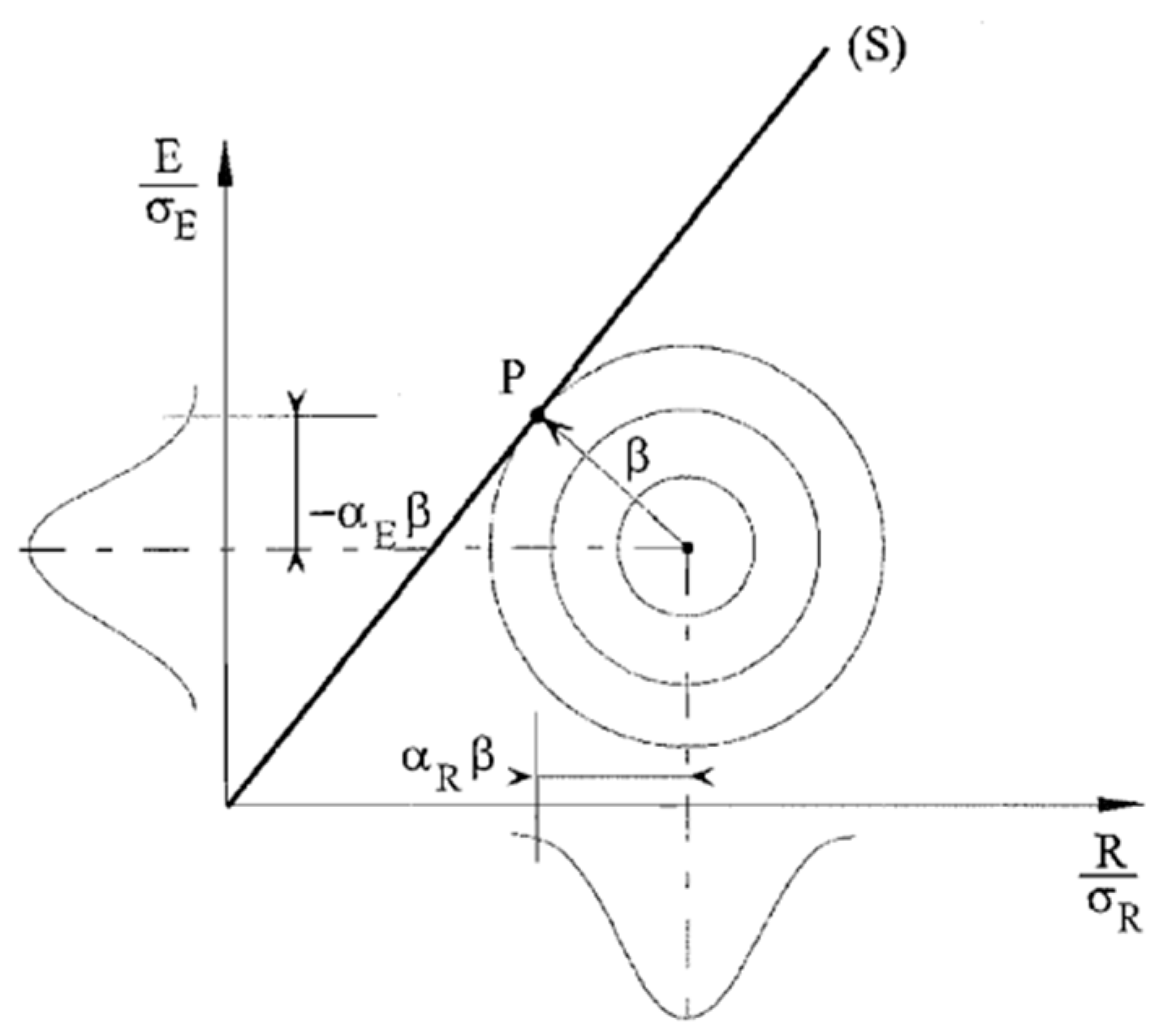
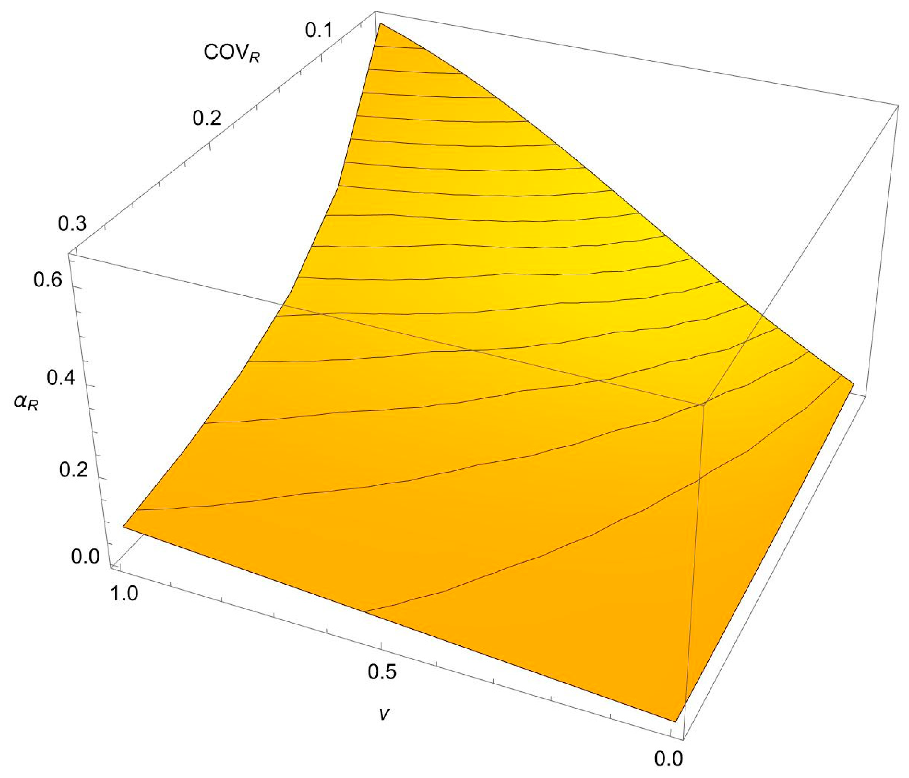
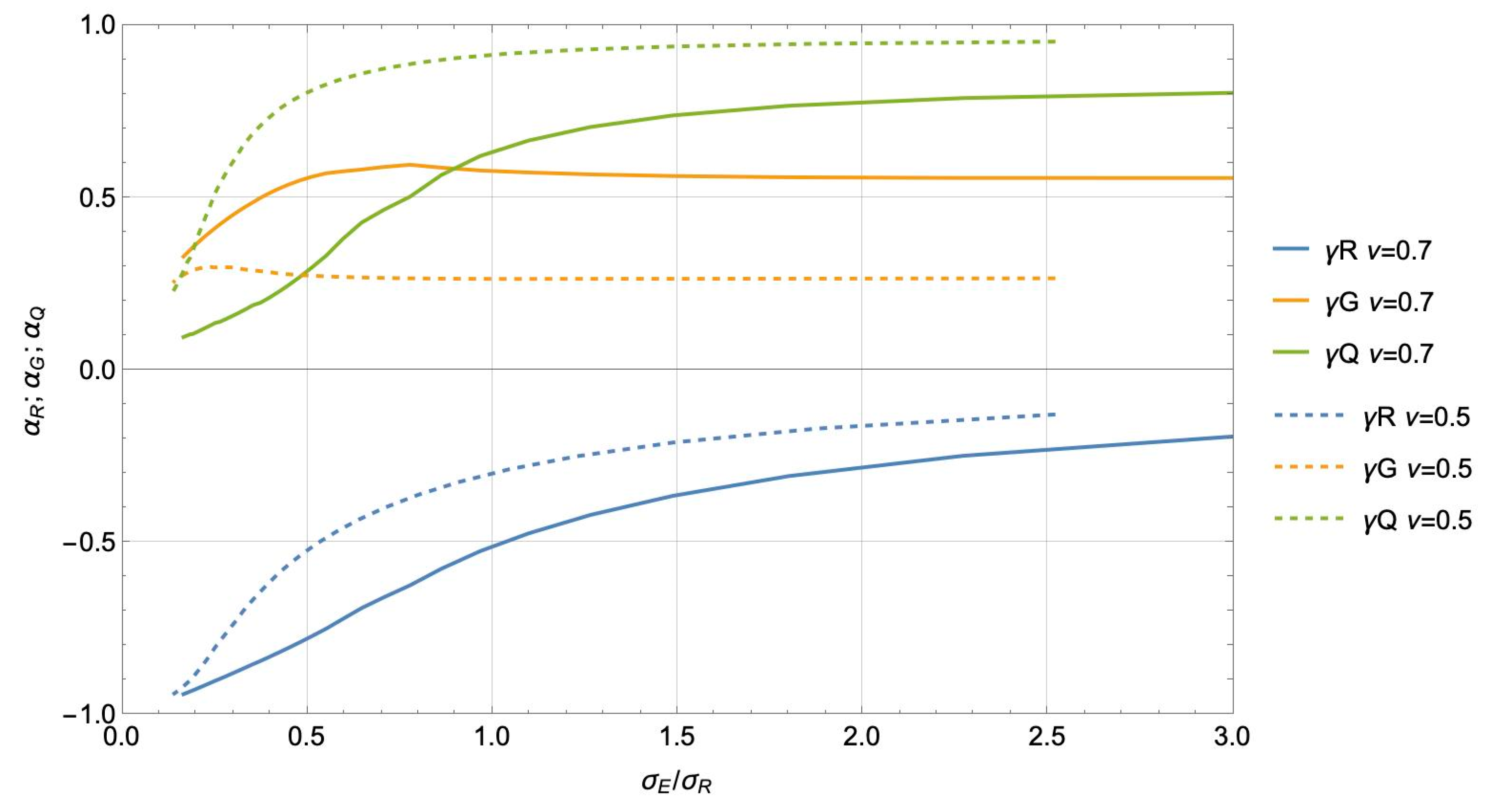
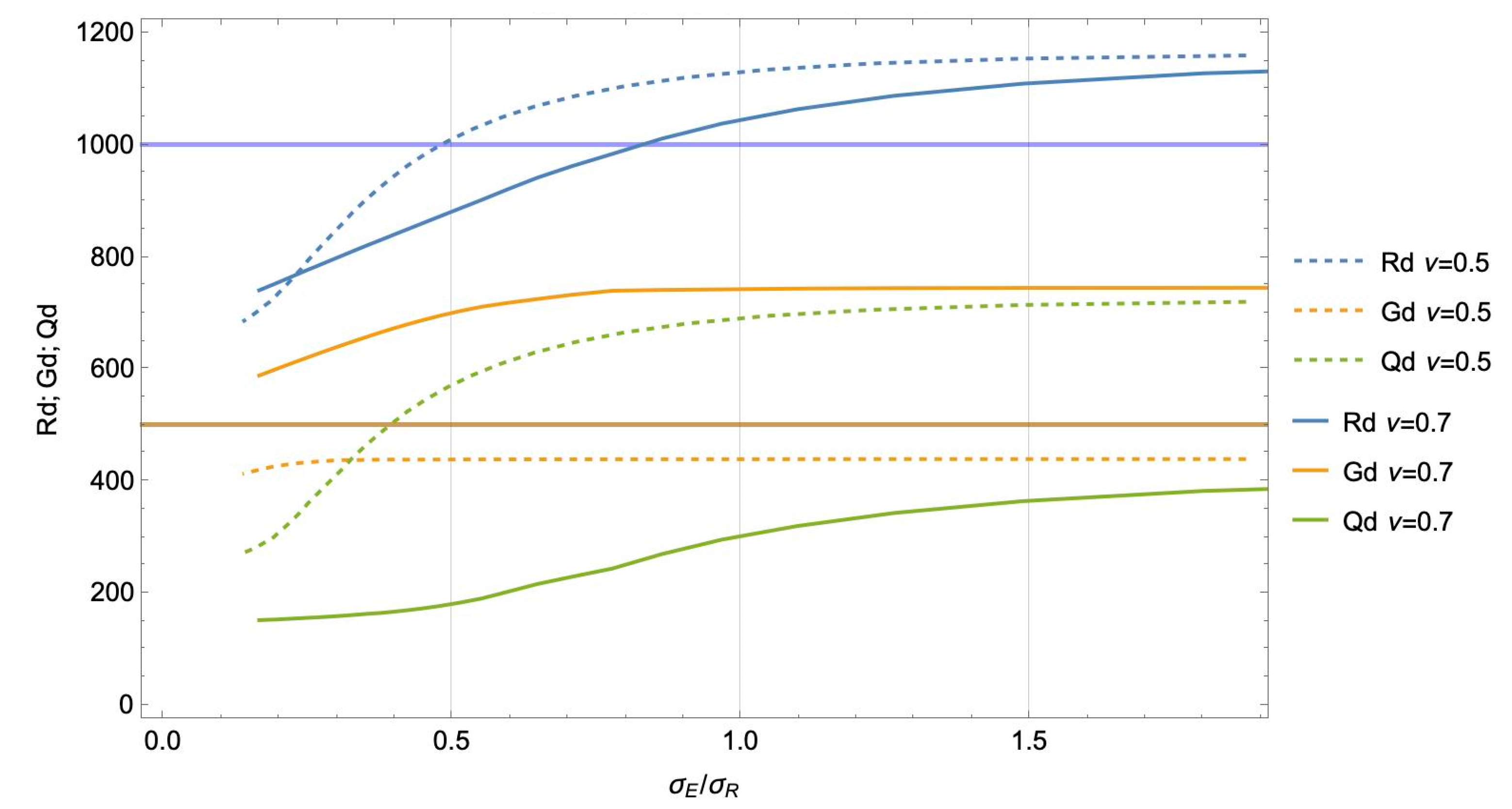
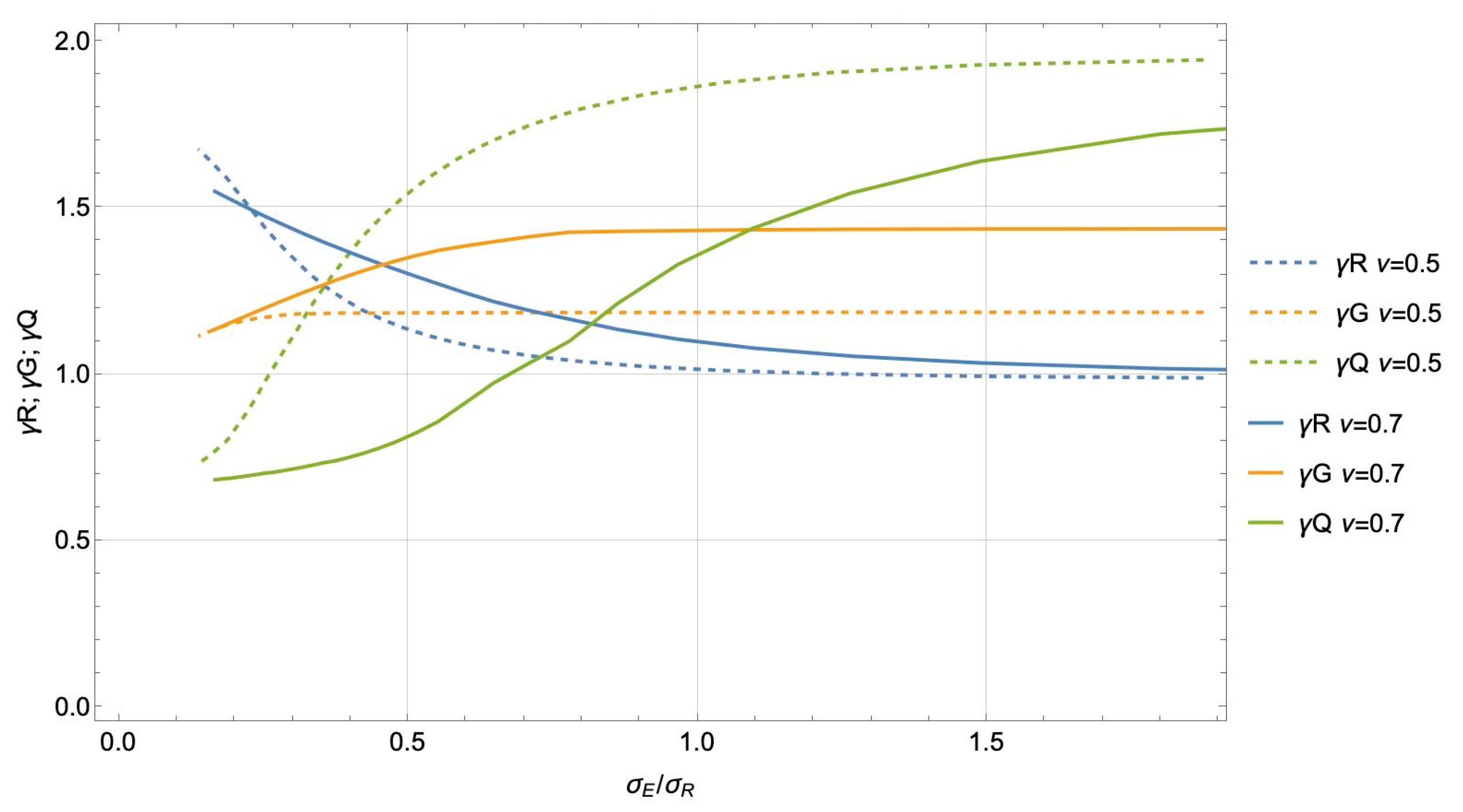
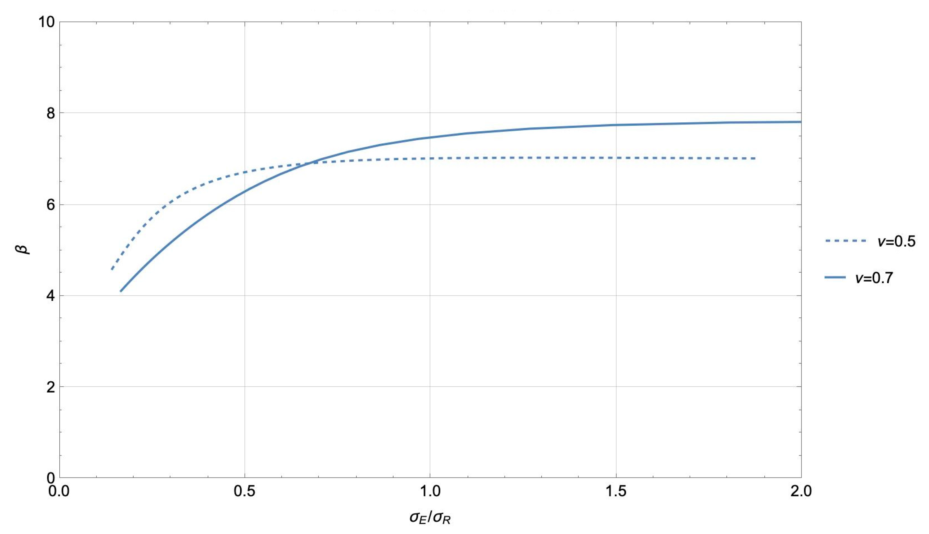
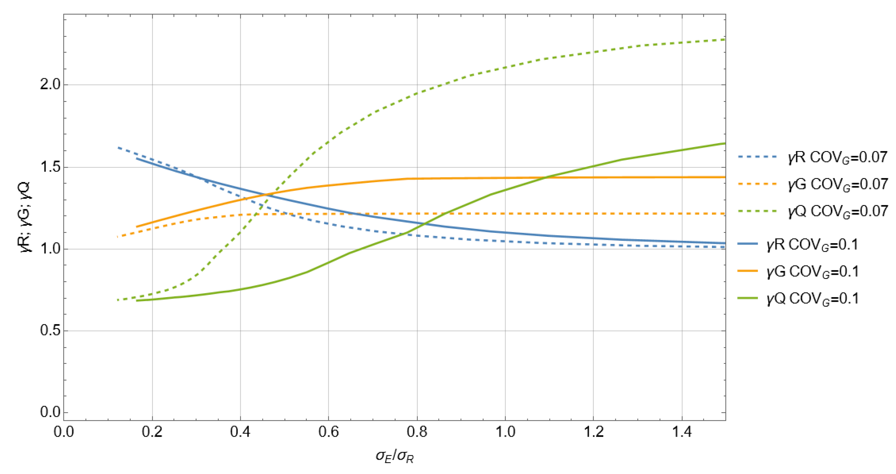
4.1. Parametric Study of the Sensitivity Factor

Using the expression for calculation of the reliability index for the considered limit state function (1), and expression for sensitivity factor for resistance (4), the parametric study is performed by setting COVQ and COVG as 0.10, and varying the percentage of dead load to total load (dead load and traffic load), ν. The graphical representation of dependence of the sensitivity factor for resistance, ratio ν, and COVR is shown in Figure 2, as a three-dimensional diagram. These values of coefficient of variations for traffic load, dead load, and resistance proved reasonable in the above literature review.
If the percentage of dead load to total load, ν, is set as 0.65 (which is a realistic value as shown in the following chapter), the sensitivity factor for traffic load, dead load, and resistance, respectively, is calculated as αQ = 0.0828, αG = 0.1537, αR = 0.9846 for the case with COVR as 0.15. These values differ significantly from the values proposed by the Eurocode as 0.7 and 0.28 for leading and accompanying actions, and 0.8 for resistance.

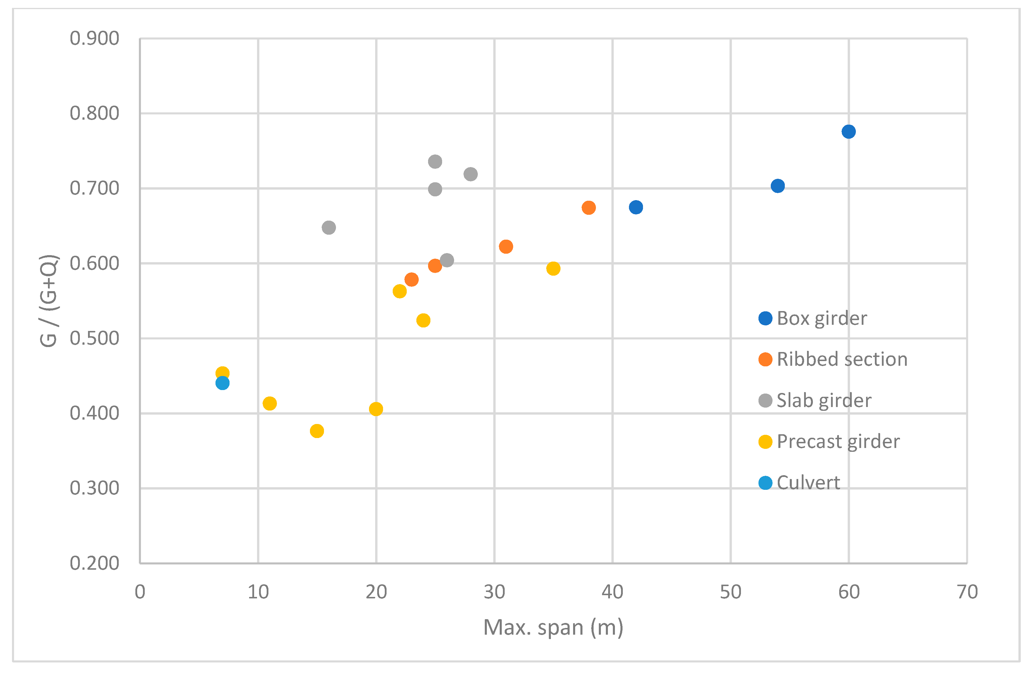
4.2. Dependence of Maximum Span of the Bridge to the Ratio of Traffic and Dead Load
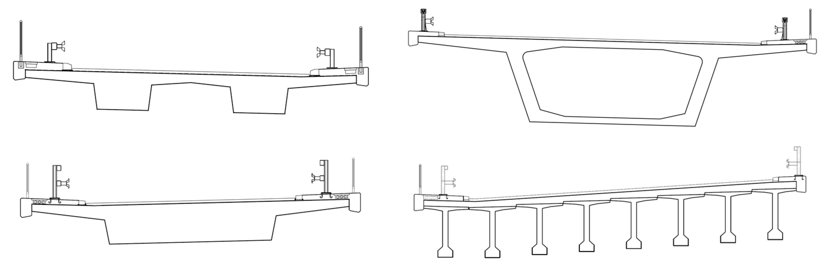
The actual bridges in whose design the first author was involved (Table 2) was investigated, and the ratio of dead load to the sum of the traffic and dead load was calculated for each bridge (Figure 3). These bridges included the following prestressed concrete bridge types (shown in Figure 4), with the range of maximum span between 7 m and 60 m:
  • slab girder bridge,
  • ribbed section,
  • box girder, and
  • precast girders.
In addition, besides the prestressed concrete bridges, one reinforced concrete culvert is included. The ratio is obtained by comparing the bending moment at support, bending moments at midspan, and shear, and taking the average of these values (weighing equally the bending moment and shear). The national load multiplier, α, for the Eurocode LM 1, used in the design of the bridges shown in Table 2, are provided in the last column of the table. As required by the National Annex used in the design of these bridges, a different set of national load multipliers, α, has been used for bridges on different routes (motorway vs more local roads). However, larger traffic loads in general ask for a larger dead load of structural components to resist the increased load, keeping the G/(G + Q) ratio relatively constant.
As can be seen from Figure 3, the ratio of dead to total load, i.e., ν, depends on the following factors:
  • Span—the longer the span, the larger the ratio, as the influence of the Tandem System (TS) part of the Eurocode Load Model 1 (LM1) decreases when compared with the uniform dead load;
  • Width of the bridge—the wider the bridge, the larger the ratio, since the wider bridge means that third lane and remaining area will be added, which are the lighter parts of the Eurocode LM1, while the dead load should increase significantly with the bridge width increase;
  • Type of the section—the slab bridge has a larger ratio ν due to disadvantageous cross-section optimization compared with the ribbed section, box section, and precast girders.
It can be concluded that the typical range of ratio ν is 0.40–0.75 for the concrete bridge. For steel bridges, ν is expected to be lower.

5. Discussion

Using fixed sensitivity factors αE and αR as −0.7 and 0.8, respectively, according to EN1990, strongly affects the probability of exceedance of the design value and calibration process of the partial factors. In the partial factor method, the partial factors are obtained by the following expression:
γ Q = x d x c
where x d is the design value (the most probably failure points), and xc is the characteristic value (in general, an arbitrary value). The design value can be calculated as:
x d = μ + β × α × σ
It is clear that the sensitivity factor is a critical input for the calculation of the partial factor. It is actually irrelevant which characteristic value one would like to choose to calibrate the load model—indeed, it can be any value—but the partial safety factor has to be calibrated accordingly. Using a safety index to calibrate the load model, and keeping the constant sensitivity factor of 0.7 gives a false impression that this choice indeed ensures a sufficient target safety index, in particular as traffic loading is not the only loading—there is a self-weight as well.
Two sets of values of the sensitivity factors are suggested for concrete bridges as a result of this study in Table 3: (a) one for bridges with the longest span between 5 m and 25 m, and (b) the other for bridges with the longest span between 25 m and 80 m. The coefficient of variation for resistance COVR of 0.10 is chosen; for the dead load and traffic load coefficient of variation, COVG and COVQ, the value of 0.10 is proposed for this purpose. For bridges with the longest span between 5 m and 25 m, ν, i.e., the ratio of dead load to total load, an equal to 0.5 has been suggested. For bridges with spans between 25 m and 80 m, ν, i.e., the ratio of dead load to total load, an equal to 0.7 has been proposed. The value of sensitivity factors for traffic loads equal to approximately 0.26 for bridges with spans between 5 m and 25 m, and 0.18 for bridges with spans between 25 and 80 m, are much smaller than the values usually used as 0.7, suggested by the Eurocode and [4,5].
In order to illustrate that the Eurocode proposed values for sensitivity factors are not appropriate, the following sample situation has been discussed. The design resistance and design load has been set to 1000, with the ratio of dead load to the sum of dead load and traffic load equal to 0.7. The corresponding characteristic values of resistance, dead load and traffic load can be then calculated as 1150, 519, and 222, respectively, by applying the Eurocode partial safety factor of 1.15 for resistance, and 1.35 for loads. Assuming normal distribution for all three random variables (resistance, dead load, and traffic load), lower 5% fractile for resistance characteristic value, nominal (expected) value for dead load characteristic value, and upper 0.1% for traffic load characteristic value, distributions for each random variable can be computed (two unknown parameters from the set of two equations for each distribution). Coefficient of variations has been assumed as 0.1 for all three variables, resistance, dead load, and traffic load. Once the distributions are determined, sensitivity factors for resistance, dead load, and traffic load are calculated using Equations (2)–(4) as 0.930, 0.350, and 0.115, respectively; using Equation (1), the reliability index is computed as 4.65. The design point, i.e., the most likely failure point, can be calculated as 781.7, which differs significantly from the starting point, Ed = Rd = 1000.
Further, a more refined parametric study to illustrate inconsistency of sensitivity factors proposed by the Eurocode was performed with the distributions usually encountered in practice—lognormal for resistance, normal for dead load, and Gumbel for traffic load. Again, the same design point Ed = Rd, the same characteristic values, the same coefficient of variations for dead load and traffic load, and the ratio of dead load to traffic load was used, as in the previous example. Distributions for each random variable was computed with the Rackwitz–Feissler algorithm (by defining a function that approximates the arbitrary distribution with the normal distribution at the most likely design point [21]). The coefficient of variation for resistance was varied and analyzed in the applicability domain of the Eurocode proposal for sensitivity factors, i.e., 0.16 < σ E / σ R < 7.16 . Plots for dependence of sensitivity factors, design point, partial safety factors, and reliability index on the ratio between standard deviation of load and resistance were plotted in Figure 5, Figure 6, Figure 7 and Figure 8. It can be concluded that sensitivity factors proposed by the Eurocode can be seen only as a rough approximation.
It is also interesting to note how partial safety factors significantly change, as the dead load coefficient of variation decreases—dead load coefficient of variation was varied as 0.07 and 0.1 in Figure 9. Generally, dead load coefficient of variation is easy to update in practice, by measuring the actual measurements of the structure on-site.

6. Conclusions

This paper shows a principle of how to accurately calculate sensitivity factors necessary for the calibration of the load model and partial safety factors—these sensitivity factors for each random variable depend on the ratio of traffic live load to dead load. The ratio of traffic live load to dead load strongly depends on the maximum center span of the bridge. It has been concluded that the calculated values of the sensitivity factor for resistance, dead load, and traffic load differ significantly from the Eurocode proposed values, which strongly influence the target safety index (and consequently, the probability of failure). It has been shown that the actual design point (i.e., the most likely failure point) with the use of the Eurocode partial safety factors differs significantly from the starting design resistance and design load; the corresponding sensitivity factors also differ from the Eurocode proposed values, which can be seen only as a rough approximation. The approach provided in this paper can be used for calculation of the sensitivity factors during the recalibration of the partial factors for new and existing bridges. Future research could include the study of typical ratios of dead load to total load for steel bridges, as this paper studied only concrete bridges in regards to this issue, although it studied the influence of this ratio to sensitivity factor in general.

Author Contributions

Conceptualization, R.H.; methodology, R.H and G.M.; validation, G.M.; formal analysis, R.H. and G.M.; investigation, R.H. and G.M..; data curation, G.M.; writing—original draft preparation, G.M.; writing—review and editing, R.H.; visualization, G.M and R.H. All authors have read and agreed to the published version of the manuscript.

Funding

This research received no external funding.

Institutional Review Board Statement

Not applicable.

Informed Consent Statement

Not applicable.

Data Availability Statement

The raw data supporting the conclusions of this article will be made available by the authors on request.

Conflicts of Interest

The authors declare no conflicts of interest.

References

  1. Eurocode EN 1992; Eurocode 2: Design of Concrete Structures. European Committee for Standardization: Brussels, Belgium, 2001.
  2. SIA. SIA 260:2003 Basis of Structural Design; Swiss Society of Engineers and Architects: Zurich, Switzerland, 2003. [Google Scholar]
  3. König, G.; Hosser, D. The Simplified Level II Method and Its Application on the Derivation of Safety Elements for Level I; CEB Bulletin: Paris, France, 1982; Volume 147. [Google Scholar]
  4. Fib Bulletin 80 Partial Safety Factor Methods for Existing Concrete Structures; fib: Lausanne Switzerland, 2016.
  5. Gino, D.; Castaldo, P.; Bertagnoli, G.; Giordano, L.; Mancini, G. Partial factor methods for existing structures according to fib Bulletin 80: Assessment of an existing prestressed concrete bridge. Struct. Concr. 2020, 21, 15–31. [Google Scholar] [CrossRef]
  6. Sjaarda, M.; Meystre, T.; Nussbaumer, A.; Hirt, M.A. A systematic approach to estimating traffic load effects on bridges using weigh-in-motion data. Stahlbau 2020, 89, 585–598. [Google Scholar] [CrossRef]
  7. Kübler, O.; Wagner, P.-R.; Girardin, B.; Friedl, H.; Schubert, M. Assessment of Railway Bridge Reliability Using Load Measurement Data. Struct. Eng. Int. 2023, 1–10. [Google Scholar] [CrossRef]
  8. JCSS. Probabilistic Model Code; The Joint Committee on Structural Safety: Zurich, Switzerland, 2001. [Google Scholar]
  9. Faber, M.H. Risk and Safety in Engineering; ETH Lecture Notes; Swiss Federal Institute of Technology: Zurich, Switzerland, 2009. [Google Scholar]
  10. Dragojević, M.; Savatović, S.; Jevtić, D.; Zakić, D.; Savić, A.; Radević, A.; Aškrabić, M. Statistical analysis of results of testing of concrete cubes. Tehnika 2019, 74, 191–197. [Google Scholar] [CrossRef]
  11. Ellingwood, B.; Galambos, T.V.; MacGregor, J.G.; Cornell, C.A. Development of a Probability Based Load Criterion for American National Standard A58; US Department of Commerce, National Bureau of Standards: Washington, DC, USA, 1980. [Google Scholar]
  12. Melchers, R.E. Structural Reliability Analysis and Prediction; John Wiley and Sons: Chichester, UK, 1987. [Google Scholar]
  13. Mirza, S.A.; MacGregor, J.G. Variability of mechanical properties of reinforcing bars. J. Struct. Div. 1979, 105, 921–937. [Google Scholar] [CrossRef]
  14. Baker, M.J. Variability in the Strength of Structural Steels-a Study in Structural Safety: Material Variablility; CIRIA: Soria, Spain, 1972. [Google Scholar]
  15. Edlund, L. Coefficients of Variation for the Yield Strength of Steel. In Proceedings of the 2nd Colloquium on Stability of Steel Structures, Final Report, Liege, Belgium, 13–15 April 1977. [Google Scholar]
  16. Galambos, T.V.; Ravindra, M.K. Properties of steel for use in LRFD. J. Struct. Div. 1978, 104, 1459–1468. [Google Scholar] [CrossRef]
  17. Kennedy, D.L.; Baker, K.A. Resistance factors for steel highway bridges. Can. J. Civ. Eng. 1984, 11, 324–334. [Google Scholar] [CrossRef]
  18. Chryssanthopoulos, M.; Manzocchi, G.; Elnashai, A. Probabilistic assessment of ductility for earthquake resistant design of steel members. J. Constr. Steel Res. 1999, 52, 47–68. [Google Scholar] [CrossRef]
  19. Nowak, A.S.; Collins, K.R. Reliability of Structures; CRC Press: Boca Raton, FL, USA, 2012. [Google Scholar]
  20. Milutinovic, G.; Hajdin, R. Evaluation of Bridge Traffic Load Model Using B-Wim Measurements in Serbia. In Proceedings of the SINARG Conference 2023, Nis, Serbia, 14–15 September 2023. [Google Scholar]
  21. Rackwitz, R.; Fiessler, B. Structural reliability under combined random load sequences. Comput. Struct. 1978, 9, 489–494. [Google Scholar] [CrossRef]
Figure 1. Design point and reliability index β according to FORM for normally distributed variables (EN1990).
Applsci 14 00985 g001
Figure 2. Three-dimensional diagram of interdependence of αR, ν, and COVR.
Applsci 14 00985 g002
Figure 3. Ratio of dead load to total load vs maximum span.
Applsci 14 00985 g003
Figure 4. Bridge types used (ribbed section (top left), box girder (top right), slab girder (bottom left), precast girder (bottom right)).
Applsci 14 00985 g004
Figure 5. Influence of standard deviation ratio on sensitivity factors.
Applsci 14 00985 g005
Figure 6. Influence of standard deviation ratio on design points (constant values being initial design values for ν = 0.5).
Applsci 14 00985 g006
Figure 7. Influence of standard deviation ratio on partial safety factor.
Applsci 14 00985 g007
Figure 8. Influence of standard deviation ratio on reliability index.
Applsci 14 00985 g008
Figure 9. Influence of COVG on partial safety factors.
Applsci 14 00985 g009
Table 1. Probabilistic model for the reinforcement yield strength [8].
VariableTypeE[X]σxCOV
[MPa]
X1Normalµ19-
X2Normal022-
X3Normal08-
A-Anom-0.02
Table 2. Bridge considered for dependence of ratio of traffic to dead load and maximum span.
Max SpanAll SpansTypeBridge Width (m)Ratio να
(LM1 Multiplier)
(m)(m)
6045, 60, 45Box girder14.80.7750.8
4232, 4 × 42, 32Box girder11.30.6751
5440, 3 × 54, 40Box girder11.30.7031
3830, 38, 38, 38, 38, 30Ribbed section10.50.6740.8
2318, 23, 23, 23, 23, 23, 18Ribbed section9.40.5780.8
2520, 25, 25, 25, 25, 25, 20Ribbed section9.40.5970.8
3122, 31, 31, 31, 22Ribbed section9.40.6220.8
2520, 5 × 25, 20Slab girder14.80.7360.8
2618, 26, 26, 26, 26Slab girder7.80.6041
2828, 28Slab girder10.50.7190.8
1616Slab girder11.30.6480.8
2525, 25Slab girder10.50.6990.8
223 × 22Precast girders11.20.5631
2017, 20, 20, 17Precast girders80.4061
3535Precast girders11.20.5930.8
2424, 24Precast girders10.50.5240.8
77Precast girders14.750.4531
1515Precast girders14.750.3761
1111Precast girders14.750.4131
77Culvert14.750.4401
Table 3. Proposal for sensitivity factors for concrete bridges.
Span RangeRatio of DeadSensitivity Factor
(m)to Total LoadαQ (traffic)αG (dead load)αR (resistance)
5–25 0.50.25610.25610.9321
25–80 0.70.15110.35250.9235
Disclaimer/Publisher’s Note: The statements, opinions and data contained in all publications are solely those of the individual author(s) and contributor(s) and not of MDPI and/or the editor(s). MDPI and/or the editor(s) disclaim responsibility for any injury to people or property resulting from any ideas, methods, instructions or products referred to in the content.

