Article

Computational Fluid Dynamics-Aided Simulation of Twisted Wind Flows in Boundary Layer Wind Tunnel

1
Undergraduate School, Chongqing University, Chongqing 400045, China
2
Key Laboratory of New Technology for Construction of Cities in Mountain Area, School of Civil Engineering, Chongqing University, Chongqing 400045, China
*
Authors to whom correspondence should be addressed.
Appl. Sci. 2024, 14(3), 988; https://doi.org/10.3390/app14030988
Submission received: 23 November 2023 / Revised: 4 January 2024 / Accepted: 15 January 2024 / Published: 24 January 2024
(This article belongs to the Special Issue City Resilience to Windstorm Hazard)

Abstract

:
The twisted wind flow (TWF), referring to the phenomenon of wind direction varying with height, is a common feature of atmospheric boundary layer (ABL) winds, noticeably affecting the wind-resistant structural design and the wind environment assessment. The TWF can be effectively simulated by a guide vane system in wind tunnel tests, but the proper design and configuration of the guide vanes pose a major challenge as practical experience in using such devices is still limited in the literature. To address this issue, this study aims to propose an approach to determining the optimal wind tunnel setup for TWF simulations using a numerical wind tunnel, which is a replica of its physical counterpart, using computational fluid dynamics (CFD) techniques. By analyzing the mechanisms behind guide vanes for generating TWF based on CFD results, it was found that the design must take into account three key parameters, namely, (1) the distance from the vane system to the side wall, (2) the distance from the vane system to the model test region, and (3) the separation between the vanes. Following the optimal setup obtained from the numerical wind tunnel, TWF profiles matching both the power-law and Ekman spiral models, which, respectively, reflect the ABL and wind twist characteristics, were successfully generated in the actual wind tunnel. The findings of this study provide useful information for wind tunnel tests as well as for wind-resistant structural designs and wind environment assessment.

1. Introduction

The wind field within the atmospheric boundary layer (ABL) is a crucial research topic because it plays an important role in the wind-resistant design of structures as well as the wind environment assessment. In most wind codes, the vertical wind profile below the gradient height, typically 200–500 m, is stipulated as follows: the wind speed increases with height following the (semi-)empirical logarithmic or power law, whilst the wind direction remains constant at all heights. However, field measurement studies have pointed out that the direction of natural wind flow within ABL may not be constant as it varies noticeably with height, which is attributed to various factors such as the Ekman effect (i.e., a combined effect of Earth’s rotation, surface friction, and pressure gradient force), atmospheric stability, terrain roughness, and baroclinity. This type of winds is referred to as the twisted wind flow (TWF, also known as the turning of winds or veering winds), and the angular difference between the wind direction at a given height and that at the gradient height is referred to as the twist angle. For instance, Mendenhall et al. [1] investigated the dependencies of the twist angle on the horizontal temperature gradient and the atmospheric stability and then proposed prediction models for the variation in the twist angle with height over land and ocean terrains. According to the long-term SODAR observations of wind characteristics in a coastal area of Japan, Tamura et al. [2] reported that the twist angle may reach about 20° within the height range of 50 to 350 m above ground. Liu et al. [3] analyzed 4766 30-min-long data segments of synoptic winds collected by a wind profiler installed in a coastal area of China, concluding that the twist angle can reach 5° to 40° over the first 1000 m above ground. Based on the field measurement data of multiple tropical cyclones collected by Doppler radar wind profilers and anemometers in Hong Kong, He et al. [4] and Shu et al. [5] suggested that wind direction generally varies 20° to 40° within the first 1000 m in height, and the twist angle is highly dependent on the terrain condition, the wind speed, and the storm type (monsoons or typhoons). Based on these field observations, it can be readily understood that the TWF may impose significant asymmetrical loads on structures, and therefore the neglect of the TWF effect may lead to inaccurate calculations of the wind loads acting on super-tall structures, including skyscrapers and gigantic wind turbines [6,7]. For instance, the variation in wind yaw angle may affect the drag and lift forces of the wind turbine blades, whilst such a TWF effect is usually neglected in turbine designs. Moreover, ignoring the TWF may also result in unreliable wind environment assessments, such as for pedestrian-level winds over complex urban and/or mountainous terrain [8].
As a widely accepted experimental approach, boundary layer wind tunnel testing is usually recommended or even mandatory for wind-resistant structural designs and wind environment assessments. To artificially replicate the TWF in conventional wind tunnels that employ passive devices (e.g., grids, spires, and ground roughness) to generate ABL winds, research efforts have been devoted over the past few decades. One of the most common approaches is to set up a guide vane system consisting of multiple vertical vanes with a curved surface to redirect the flow at the outlet of the wind profile development region (i.e., where the passive devices are installed). Given a properly designed guide vane system, the wind flow can be twisted to achieve the desired orientations at various heights, so that the flow in the downstream model test region follows a profile that has both the speed and direction varying with height in the required manner. One of the first attempts was made by Prof. Flay and his research group from the University of Auckland, who evaluated the aerodynamic performance of downwind yacht sails by installing plastic vanes [9]. Despite the drawbacks, such as high turbulence intensities and dips in mean wind speeds at regular heights, this guide vane system delivered promising test results that well agreed with the data obtained by numerical simulations and field measurements. The successful application of this guide vane system has not only spurred studies in sail aerodynamics [10,11], but has also garnered attention from the research field of civil engineering. In recent years, a few wind tunnel tests have been conducted to investigate the TWF effect on structures and the wind environment [12,13] In particular, Tse et al. [8] fabricated five wooden vanes to simulate the TWF at the pedestrian-level height caused by mountainous and densely built city terrain, indicating that the TWF noticeably modifies flow features such as asymmetric wind speed distributions and reduced wind speed near an isolated building or building groups. Liu et al. [14] generated two TWFs with the characteristics of thousand-meter-high ABL winds using four vanes and pointed out that the value of wind load applied to a super-tall building under the TWF effect highly depends on the total twist angle instead of being a specific value. Yan et al. [15] developed two one-piece molded-fiberglass vanes to investigate the TWF effect on a typical super-tall building, highlighting that the TWF significantly affects the distribution of extreme cladding pressures and local wind loads. Nevertheless, the wind tunnel investigation of the TWF is still lacking, and one of the major difficulties it encounters is the design of a proper guide vane system.
As an alternative approach to investigating the wind effect, numerical simulation using computational fluid dynamics (CFD) techniques has also been widely adopted in numerous studies. Compared with typical wind tunnel testing, numerical simulations have prominent advantages, such as the detailed illustration of flow fields, which is especially important to the investigation of complex flow structures, e.g., the TWF. To numerically simulate the pedestrian-level wind field under the TWF effect, Weerasuriya et al. [16] introduced new inflow boundary conditions to model the wind speed profiles of the TWF. Feng et al. [17] and Lu and Li [18] incorporated the Coriolis force term in the momentum equations to numerically generate the TWF profiles, so that the influence of the Coriolis force on the TWF could be clearly demonstrated by comparing the TWF profiles with the reference profiles generated without this term. However, most of these studies generated the TWF profiles directly as the inlet boundary condition, and thus they hardly provided useful advice for the design of guide vane systems in wind tunnel tests. On the other hand, by combining advanced CFD techniques with the skills and experience in wind tunnel testing accumulated over the decades, the concept of a numerical wind tunnel has emerged. A numerical wind tunnel mimics its physical counterpart by setting the inlet boundary condition as a uniform flow and creating models of passive devices (e.g., grids, spires, and ground roughness) in the computational domain, allowing the desired ABL wind profile in the downstream area to be generated in a similar manner to that in an actual wind tunnel. Aly and Bitsuamlak [19] established a numerical wind tunnel using models of spires and ground roughness, which allowed them to test solar panels at various geometric scales with ease. Phuc et al. [20] modeled spires and ground roughness to generate ABL winds, suggesting that the simulation results of wind speed and turbulence intensity well agree with those obtained from wind tunnel tests. To investigate the performance of a novel device for the wind tunnel simulation of transient gust-front outflow, Le et al. [21] created a numerical wind tunnel and analyzed the flow field generated by this device in detail. Given the successful applications of numerical wind tunnels in the literature, it is reasonable to assume that one can explore various experimental setups in a numerical environment through CFD techniques to identify the optimal one, which can then be implemented in an actual (i.e., physical) wind tunnel test. Such an approach, known as CFD-aided wind tunnel testing, is highly beneficial for testing novel experimental devices for which prior experience is limited, enabling researchers to gain insights into the performance of different designs of this device and to select the optimal design for the tests in the actual wind tunnel.
In this study, a procedural framework will be proposed to effectively optimize the wind tunnel experimental setup for TWF simulations utilizing CFD techniques, with a particular focus on the design of a guide vane system. The present paper contributes to the improvement in experimental and numerical simulation techniques for the TWF, promoting the application of the CFD-aided wind tunnel testing approach in the investigation of non-conventional wind flow. This paper is organized as follows: Section 2 proposes the procedural framework for the optimization of a wind tunnel setup; Section 3 presents the preparation stage of the framework, including the selection of target wind profiles and the basic information of the wind tunnel setup; Section 4 presents the development stage, including the establishment of a numerical wind tunnel using CFD techniques and the optimization of the design of a guide vane system; Section 5 describes the closeout stage, which finalizes the optimal experimental setup in the actual wind tunnel and validates the results, followed by the concluding remarks in Section 6. A nomenclature for the main parameters involved in this study is presented below for ease of reading.

2. Procedural Framework

To generate the desired TWF in the boundary layer wind tunnel efficiently and properly, this study proposes a procedural framework for the configuration of the wind tunnel experimental setup using CFD techniques. The general approach is to first preliminarily determine the experimental setup for the generation of the TWF in the numerical wind tunnel established using CFD techniques and, subsequently, optimize the experimental setup by conducting tests in the actual (i.e., physical) wind tunnel. Figure 1. illustrates the procedural framework of the CFD-aided wind tunnel simulation of the TWF in the form of a flowchart, demonstrating that the framework consists of three stages, namely, the preparation stage, the development stage, and the closeout stage. The steps involved in each stage are described as follows:

2.1. Preparation Stage

Step A determines the target wind profiles of the TWF as well as the passive devices needed to generate these profiles, such as grids, spires, ground roughness, and guide vanes. To describe the TWF comprehensively, this study proposes three target profiles: (1) the longitudinal mean wind speed profile, U ( z ) , where z denotes the height; (2) the longitudinal turbulence intensity profile, I u ( z ) ; and (3) the twist angle profile, θ T ( z ) .

2.2. Development Stage

Step B validates the CFD setup for the TWF simulations by comparing the results obtained from the numerical wind tunnel with those from an actual one. The validation involves the selection of the turbulence model, the computational domain, the grid scheme, and the solution strategy in CFD. Only the CFD setup that leads to a simulation error, e r W T , C F D , below the preset threshold, e r lim , will be adopted for further steps (i.e., e r W T , C F D < e r l i m ). To ensure sufficient accuracy of the CFD simulations, this study sets the threshold e r l i m at 20%. Notably, this step aims only to validate the CFD setup, and therefore the TWF generated at this step is generated without the characteristics of ABL winds.
Step C optimizes the design of the guide vane system to generate the desired twisted wind field. The design includes two aspects, including (1) the geometrical shape of the vane and (2) the spatial configuration of the vanes. The shape of a guide vane is quantified by two terms, namely, the variation in the twist angle with height, θ vane ( z ) , and the total height of the guide vane, H vane . As for the spatial configuration, the location of the i-th guide vane is denoted by ( x i , y i ) vane using a Cartesian coordinate system. By adjusting the above parameters of the guide vanes in the numerical wind tunnel, a TWF over the entire model test region, typically the turntable area, can be generated.
Step D incorporates the ABL wind characteristics into the TWF generated at Step C. This is achieved by adding the conventional passive devices (e.g., grids, spires, and ground roughness) into the numerical wind tunnel. Multiple parameters, such as the amount, dimensions, and locations of these conventional devices, are carefully adjusted to generate the desired TWF. The setting up of the conventional devices can usually be accomplished with ease based on the experience gained from the actual wind tunnel.
Step E evaluates the performance of the experimental setup established at the previous step. If the error for numerical simulation (i.e., the difference between the simulation results and the target values), denoted by e r obj , CFD , is lower than the preset threshold of e r lim = 30% (proposed based on practical experience), the current experimental setup will be adopted for the next step in the closeout stage. Otherwise, the procedures in Steps C and D will be carried out again until the requirement e r obj , CFD   <   e r lim is met.

2.3. Closeout Stage

Step F finalizes the experimental setup in the actual wind tunnel based on the results obtained from its numerical counterpart. Due to the inevitable errors in numerical simulations, it is a necessity to replicate the experimental setup in the numerical wind tunnel in its physical counterpart and then refine the setup with minor adjustments. In this study, the simulation error in the actual wind tunnel, e r obj , WT , is controlled to be below 10%.
In the following sections of this paper, each step of the procedure framework stated above will be carried out, and the results will be discussed in detail.

3. Preparation Stage

3.1. Target Wind Profiles

As pointed out by previous full-scale field measurement studies [3,5,8,22], the profiles of the TWF are highly dependent on the meteorological background and the local terrain effect. A variety of wind profile models have been proposed to quantitatively describe the TWF caused by different mechanisms. This study selects four widely recognized models of twisted wind angle for discussion, namely, (1) the Ekman spiral model for the TWF induced by Coriolis force [3,23], (2) the inverse proportion model [3] and the exponential law model [8] for the TWF induced by mountainous terrain, and (3) the logarithmic law model [4] for the TWF induced by tropical cyclones over coastal areas.
In particular, for the Ekman spiral model, the profiles of the wind speed in the longitudinal and lateral directions, denoted by u and v , respectively, and the twist angle, θ , are expressed by:
u z = u g 1 e z h E cos z h E v g e z h E sin z h E
v z = v g 1 e z h E cos z h E u g e z h E sin z h E
θ z = tan 1 v ( z ) u ( z )
where u g and v g are the gradient wind speeds in the longitudinal and lateral directions, respectively, and h E is the Ekman height determined by the Coriolis parameter and the turbulence viscosity coefficient.
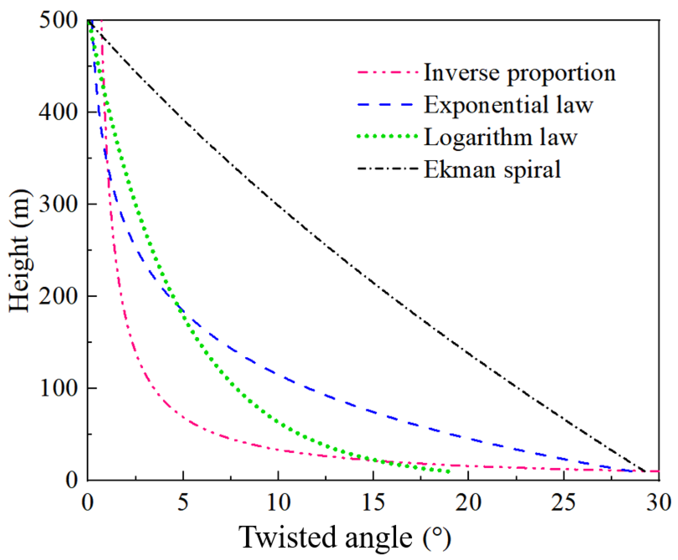
By setting the maximum twist angle at the ground level at 30° and that at a height of 500 m at 0°, Figure 2 depicts the twist angle profiles obtained from the above four models. It is readily observed that the twist angle following the inverse proportion model rapidly drops to a value below 5°, which is a very small angle corresponding to negligible TWF effects, as the height reaches 100 to 200 m, and those following the exponential law and the logarithm law models decrease to approximately 5° at a height of 200 m. In contrast, the twist angle expressed by the Ekman spiral model remains higher than 5° until the height reaches 400 m, indicating that the twisted wind effect represented by such a model is much more prominent than those represented by the three other models. Therefore, to consider the most prominent twisted wind effect for conservative purposes, this study selects the twist angle profile expressed by the Ekman spiral model as the target profile for the generation of the TWF in the wind tunnel.

3.2. Wind Tunnel Setup

A series of tests were conducted in the Wind Tunnel Laboratory at the School of Civil Engineering, Chongqing University. The test section is 2.4 m × 1.8 m (breadth × height) in size, and the turntable is 2.0 m in diameter. Multiple passive devices were employed in the wind tunnel to generate the target TWF profile that follows the Ekman spiral model. Different combinations of spires and ground roughness elements, with the dimensions indicated in Figure 3, were available to generate the ABL wind profiles. In this study, the target profiles of wind speed and turbulence intensity are expressed as follows:
u z = u u g α
I u z = I u I u , g α 0.1
where u g and I u , g denote the longitudinal wind speed and turbulence intensity at the gradient height, respectively, and α denotes the power-law exponent, which is taken as 0.12 in this study.
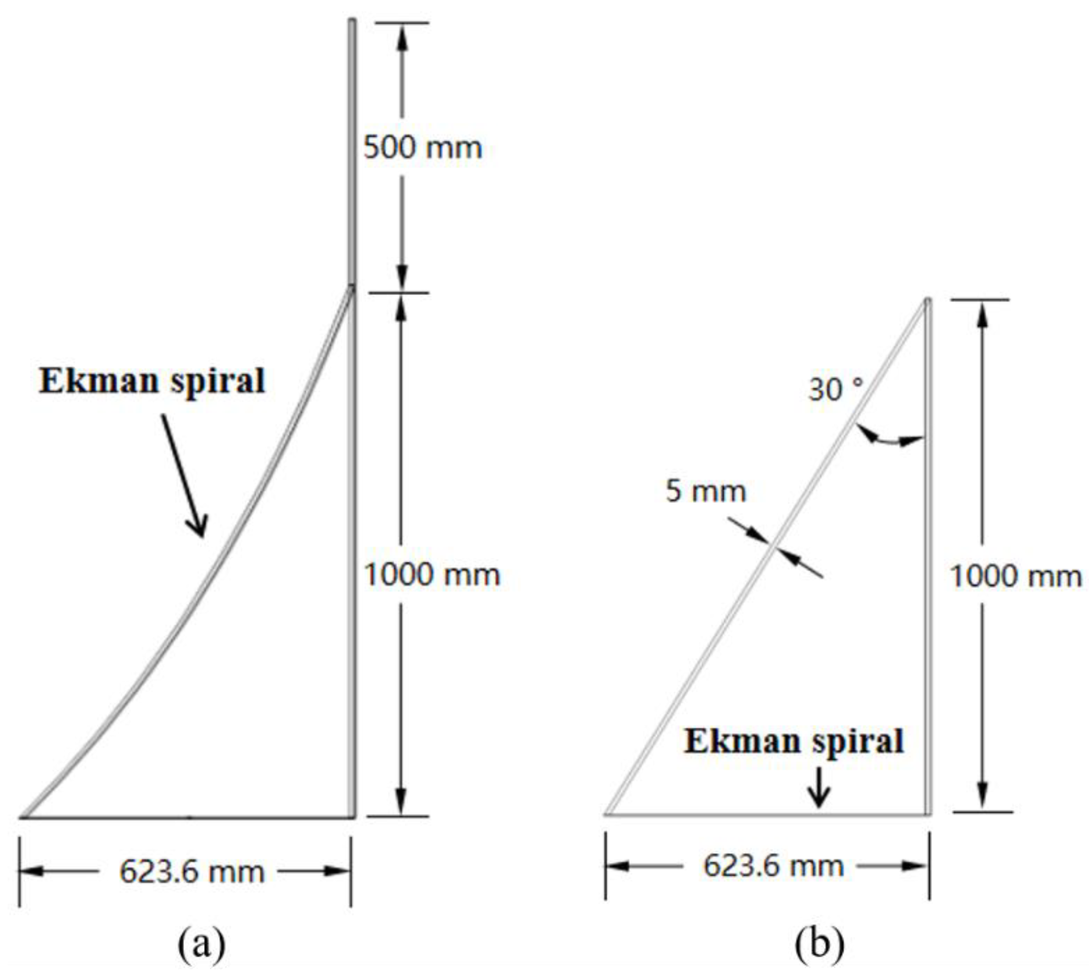
On the other hand, the TWF was generated using the guide vane system shown in Figure 4. This system comprises two identical vanes made of 10 mm thick fiberglass molded into a single piece. Each guide vane is of a total height of 1.5 m and consists of two sections, as plotted in Figure 5, namely, a twist section ranging from ground level to 1.0 m in height and a transition section from 1.0 m to 1.5 m. The leading edge of the twist section is straight, whilst the trailing edge is curved to form a guide angle varying with height to redirect the approach flow. Since the Ekman spiral model has been selected in this study as discussed above, the trailing edge is curved following Equation (3) with a twist angle of 30° at ground level and 0° at a height of 1.0 m. The transition section is in the shape of a straight board to avoid altering the flow direction and to prevent the unfavorable eddies generated at its leading edge from reaching the downstream area. At the preparation stage, the two vanes were positioned as shown in Figure 6a, i.e., one vane was installed on the right side of the wind tunnel (as observed in Figure 4) with its trailing edge 850 mm from the side wall, and the other vane was installed on the left side with a separation of 900 mm between the vanes.
To comprehensively measure the flow field generated in the wind tunnel, a Cobra probe (Turbulent Flow Instrumentation Pty. Ltd., Victoria, Australia) was deployed to measure the winds over five different locations within the model test region (i.e., turntable), indicated as Points A to E in Figure 6a. The winds were measured at 13 different heights ranging from 50 to 1050 mm, as shown in Figure 6b, i.e., the heights from 50 to 250 mm with intervals of 50 mm and from 250 to 1050 with intervals of 100 mm. By setting the geometric scale as 1:500, the above height range in the model scale corresponds to 25 to 525 m in full scale. The measurements were performed for 30 s at each height. The sampling frequency was set at 625 Hz, which is adequately high to capture the turbulence characteristics of the flow. To obtain accurate mean wind speed and direction profiles, the measurements were repeated three times at each height, and the average values were adopted.
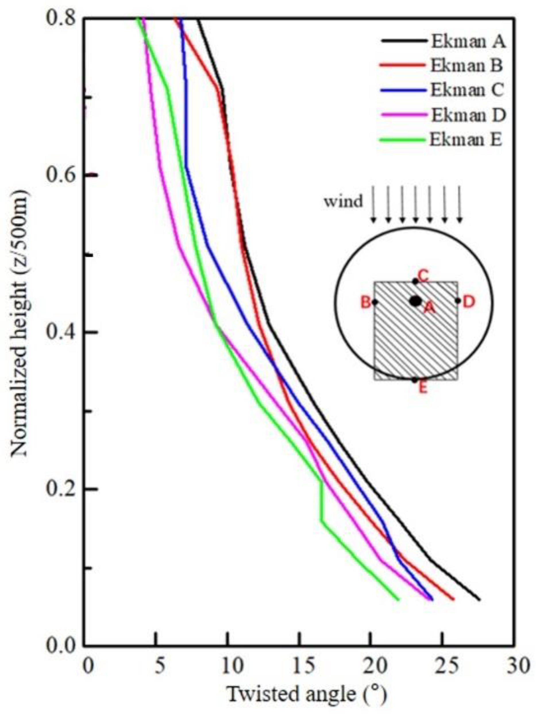
Figure 7 depicts the twist angle profiles measured over Points A to E. These profiles generally match each other, suggesting that the TWF generated by the vanes was distributed over the model test region in a uniform manner (i.e., flow speed and direction at the same height are similar within the region). It is also observed that the measured maximum twist angles were slightly below 30°, which is attributed to the inevitable attenuation of the twisting characteristic along the flow direction [8]. Overall, the variations in the measured twist angles decreased slowly with height following the Ekman spiral model, indicating that the selection of the shape of the guide vanes used in this study was reasonable.

4. Development Stage

4.1. Establishment of Numerical Wind Tunnel

4.1.1. CFD Setup for Numerical Wind Tunnel

In the CFD simulation, the complex fluid dynamics issues can be simplified for numerical resolution through the Navier–Stokes (N-S) equations. By neglecting the temperature effect, a closed set of governing equations is formed by the continuity equation and the momentum conservation equation. In this study, both the Reynolds-Averaged Navier–Stokes (RANS) model and the Large-Eddy Simulation (LES) model are utilized for the CFD simulations.
Vortex filtration is involved in the LES model by considering the feature grid size. Large-scale vortices are solved directly by the N-S equation, and small-scale ones are solved by the sub-grid scale model. The governing equations in the instantaneous state after filtration can be expressed as:
u ~ i x i = 0
u ~ i t + u ~ j u ~ i x j = p ~ x i + 1 R e 2 u ~ i x j 2 τ i j x j
where τ i j is the sub-grid scale stress, given by τ i j = ρ u i u j ~ ρ u ~ i u ~ j to make the equations closed.
The standard Smagorinsky sub-grid model [24] is adopted in this study as the LES turbulence model, expressed as:
τ i j 1 3 τ k k δ i j = 2 μ t S ~ i j
μ t = ( C s Δ ) 2 S
S ~ i j = 1 / 2 u ~ i / x j + u ~ j / x I
S = 2 S ~ i j S ~ i j
Δ = ( Δ x Δ y Δ z ) 1 3
where μ t is the dynamic viscosity in the sub-grid scale; S is the velocity scale; Δ x , Δ y , and Δ z are the grid size in the x, y, and z directions, respectively; and C s is the Smagorinsky constant taken as 0.1 in the present study.
On the other hand, statistics are used in the RANS approach to represent turbulence flow as time-averaged and fluctuating parts. When the N-S equations are averaged, the instantaneous velocity is regarded as the sum of the average velocity and the fluctuation velocity. The equations are expressed below:
u ¯ i x i = 0
u ¯ i t + u ¯ j u ¯ i x j = 1 ρ p ¯ x i + x j υ u ¯ i x j + u ¯ j x i u i u j ¯
where ρ is the air density; I and u j are the wind velocity components; υ is the coefficient of kinetic viscosity; and I i and x j are the coordinates vector of corresponding velocity components. An additional term, namely the Reynolds stress ρ u i u j ¯ , is contained in the incompressible N-S equations for the RANS simulation. To make the equations closed, several turbulence models were proposed based on different assumptions about this term, including the Standard k-ε model [25], the RNG k-ε model [26], the Realizable k-ε model [27], the Standard k-ω model [28], and the SST-k-ω model [29].
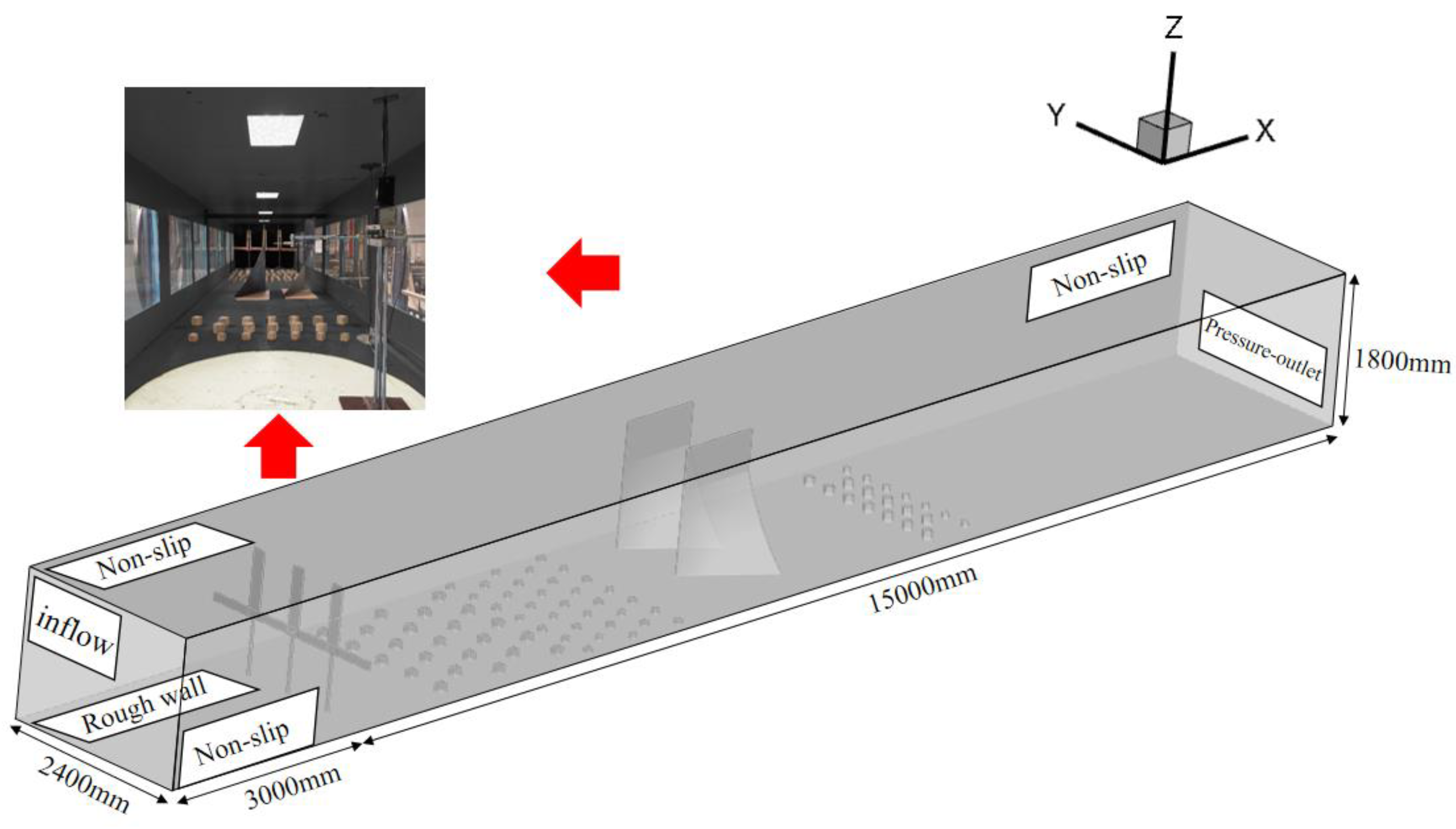
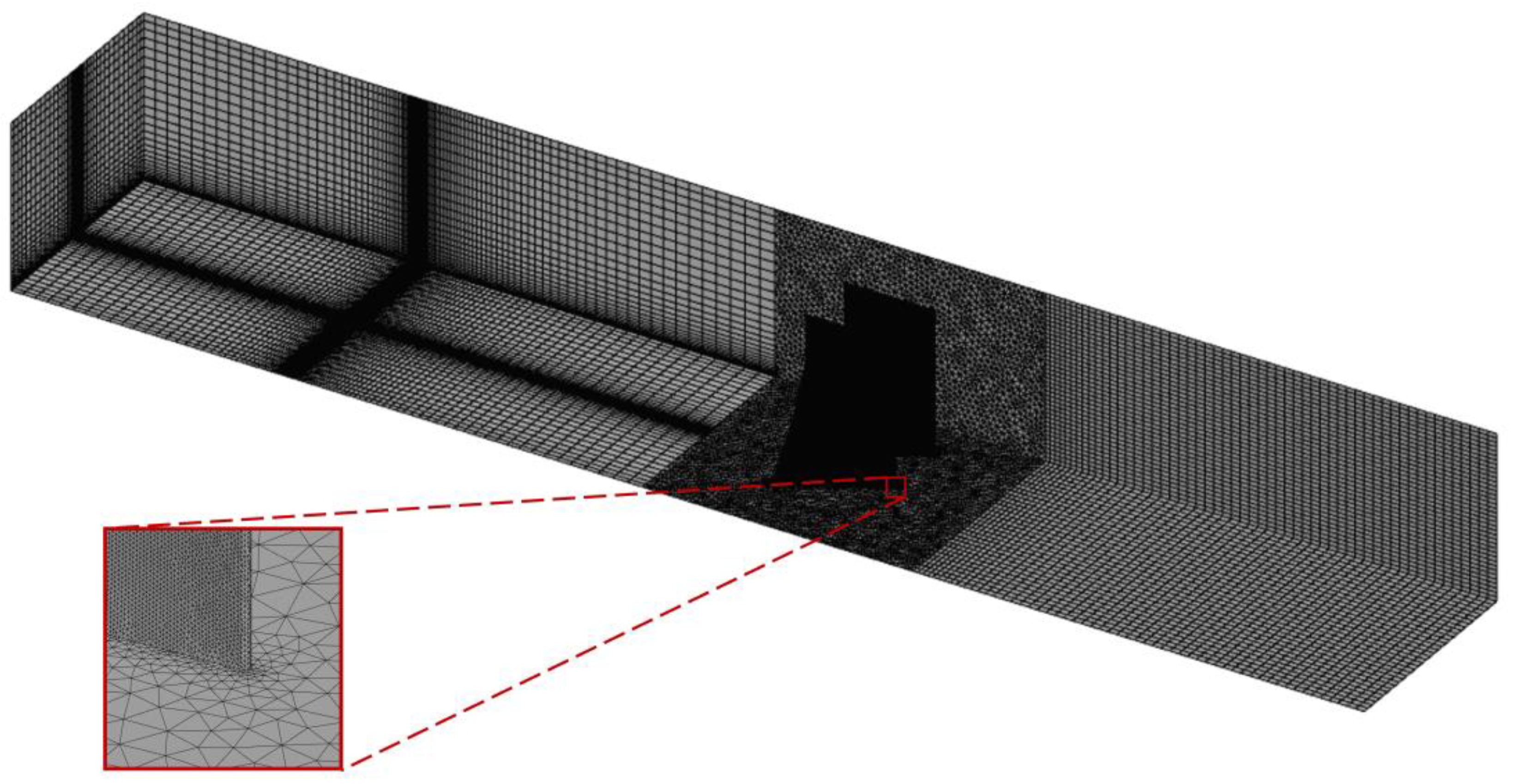
Using CFD techniques, a numerical wind tunnel was established as a replica of the wind tunnel at Chongqing University introduced in Section 3. As shown in Figure 8, the dimensions of the numerical wind tunnel were identical to those of its physical counterpart, and all passive devices available for this study, as shown in Figure 3, were also modeled numerically. As for the boundary conditions, the computational domain employed a velocity inlet and a pressure outlet, the floor was set as a rough wall, and all other surfaces, including the surfaces of the experimental devices, were set as non-slip walls. A mixed-grid scheme was adopted for both the RANS and LES simulations. The structured grids were generated near the inlet and outlet, while unstructured grids were employed in the region where the passive devices were located. The unstructured cell region and the structured cell regions were connected by the interior face.
As for the solution strategy for the RANS and LES methods, the Semi-implicit Method for Pressure-linked Equation (SIMPLE) algorithm was used to resolve the pressure–velocity coupling equation. For the RANS, the second-order upwind scheme was used to discretize the turbulence kinetic energy equation and the turbulence dissipation rate equation. For the LES, the second-order upwind scheme was applied to handle the non-linear convection term of the momentum equation, while the bounded central differencing scheme was used for the momentum equation. Additionally, the second-order implicit scheme was adopted for time discretization. To enhance computational efficiency and robustness, the RNG k-ε model was initially utilized to obtain an initial result for the subsequent LES simulation. The time step in the LES simulation was set to 0.001 s, ensuring that the Courant number remained less than 1 throughout the entire simulation.
A hyper-threading workstation with 96 CPUs and an Intel Xeon Platinunm 8269 @2.50 GHz processor at the School of Civil Engineering, Chongqing University, was used for running the CFD simulations. The calculations were conducted with the finite volume method (FVM) based on ANSYS FLUENT 19.2.

4.1.2. Validation of CFD Setup

The numerical model of the guide vanes was constructed in the computational domain for the subsequent RANS simulations. Measurement points were positioned in the region of interest to monitor and record the time history of flow velocity data. Based on the grid strategy presented above, Figure 9 presents the meshing grids of the computational domain for the validation case discussed in this section, with a close-up image of the leading edge of a guide vane to show the details. The Grid Convergence Index (GCI) method proposed by Roache et al. [30] was employed for the grid independence examination. Table 1 presents the average wind speed at a height of z = 0.85 m above the center of the model test region, showing that the relative error between the simulation results obtained using the basic grid (4.24 × 10⁶) and those obtained using the refined grid (7.34 × 10⁶) was only 1.01%. Considering the trade-off of accuracy and computational efficiency, the basic grid can be deemed suitable for carrying out the subsequent numerical simulation.
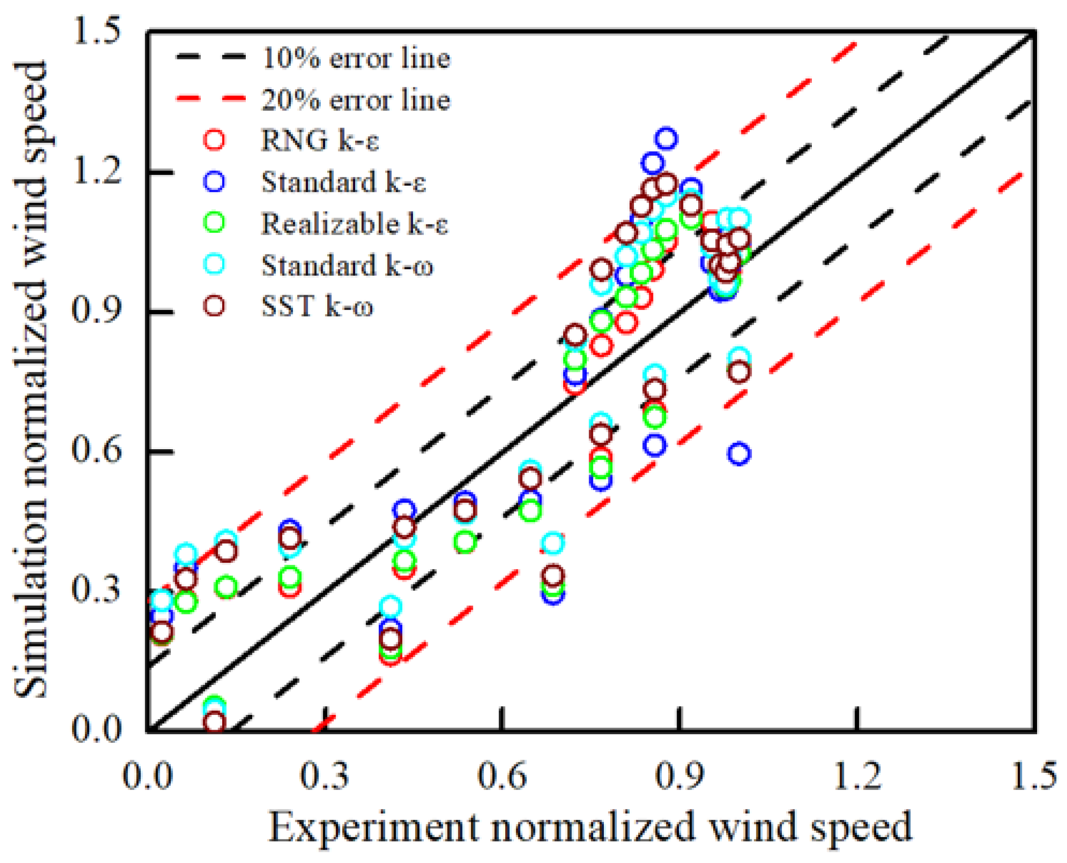
To simulate the flow with satisfactory accuracy through RANS, five turbulence models were examined, namely, RNG k-ε, Standard k-ε, Realizable k-ε, Standard k-ω, and SST k-ω. Figure 10 compares the mean wind speeds obtained by RANS simulations using these five models with those obtained by actual wind tunnel testing, with the curves representing the 10% and 20% errors from the experimental results. It is observed that the predictions by the RNG k-ε model exhibited the lowest deviation from the experimental data with relative errors below 15%; therefore, this model was selected for subsequent RANS simulations.

4.2. Optimization of Guide Vane Configuration

4.2.1. Distance from Side Wall

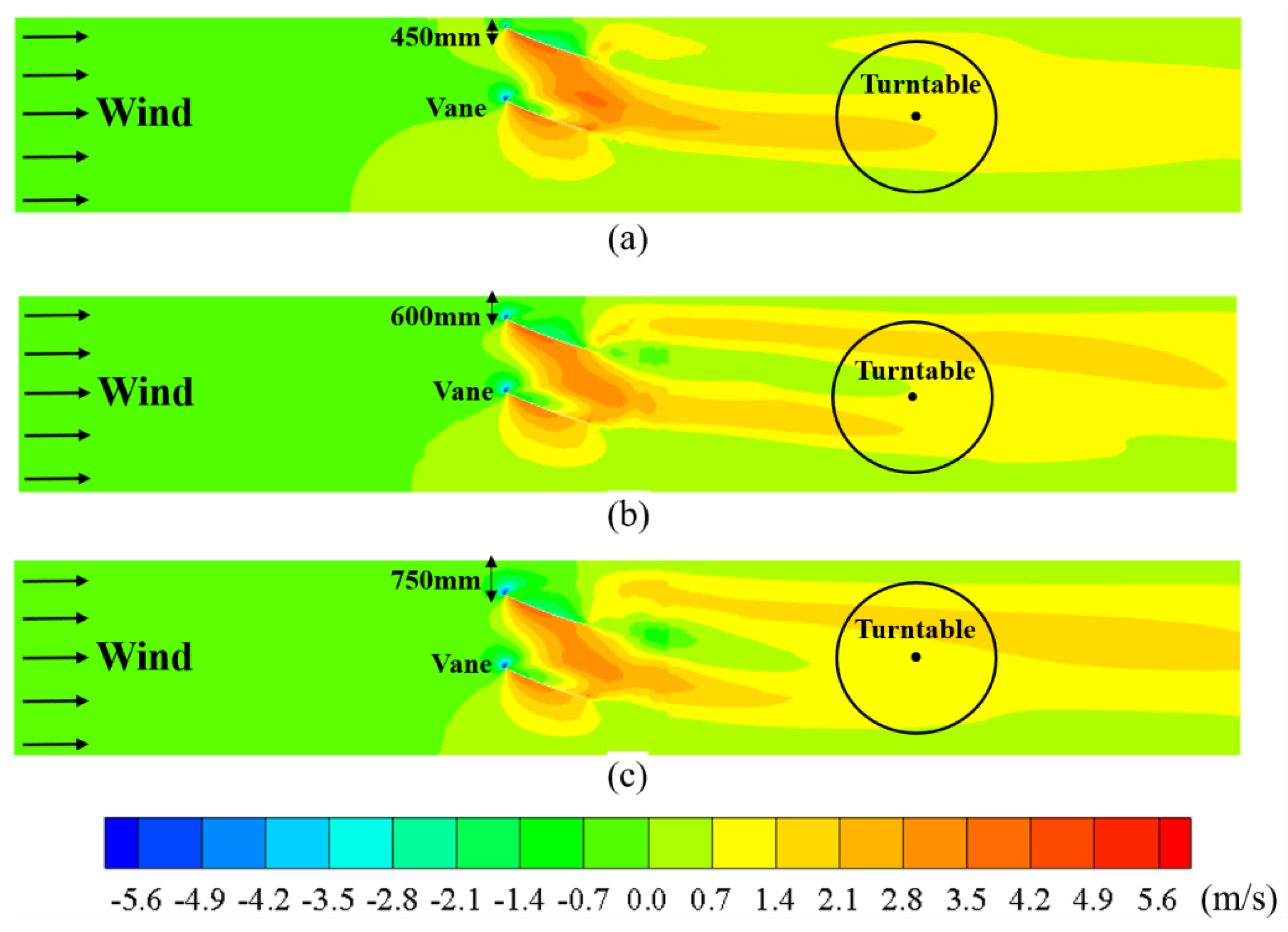
To obtain the optimal configuration of the vane system in the numerical wind tunnel, this study first investigates the changes in flow pattern caused by different distances between the leading edge of the left vane (viewed along the flow direction as shown in Figure 4) and the side wall, denoted by d v a n e , w a l l herein. Figure 11 illustrates the distribution of mean lateral wind speed in the wind tunnel at z = 0.3 m generated by the left vane positioned at d v a n e , w a l l = 450, 600, and 750 mm, while the spacing between the vanes was kept constant at 700 mm. The mean lateral wind speed within the downstream region of the left vane in Figure 11a is considerably lower than those in Figure 11b,c, which is evidently attributed to the blockage in the area near the leading edge of the left vane, i.e., the flow has to slow down when it passes through such a narrow gap d v a n e , w a l l = 450 mm. Such blockage is alleviated as d v a n e , w a l l increases and fully disappears as d v a n e , w a l l reaches 750 mm. Hence, d v a n e , w a l l = 750 mm is selected for further numerical simulations in the following steps.

4.2.2. Spacing between Guide Vanes

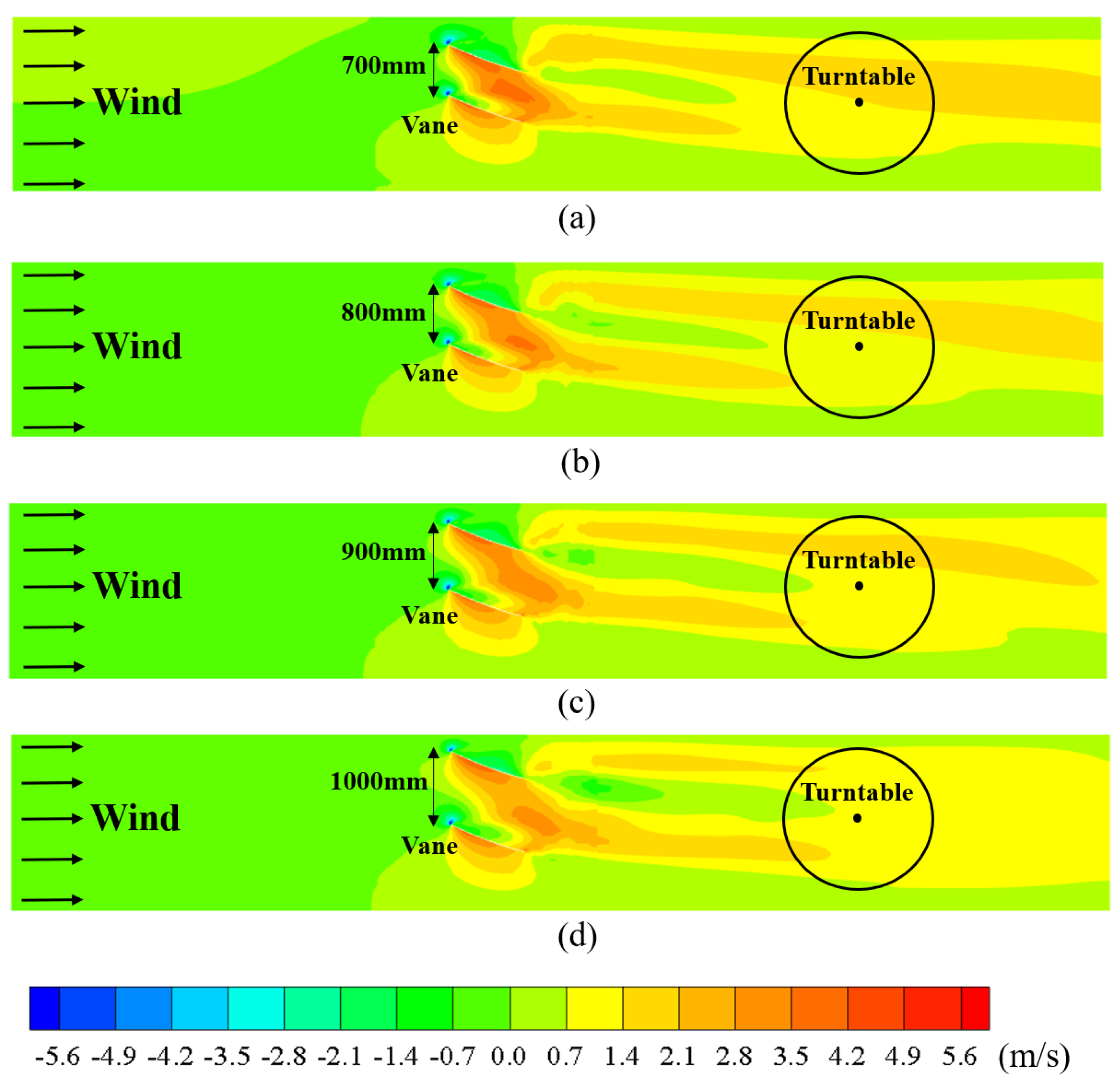
After determining d v a n e , w a l l = 750 mm, the next step is to identify the optimal spacing between the two vanes. Figure 12 shows the distribution of the lateral wind speed at z = 0.3 m with d v a n e , w a l l = 750 mm and the spacing between the vanes, denoted by d v a n e , v a n e herein, ranging from 700 to 1000 mm with intervals of 100 mm. The figure shows that a so-called “low-speed area”, where the mean lateral wind speed is below 0.7 m/s (colored in green), is formed in the downstream region of the vanes. The length of the low-speed area increases with d v a n e , v a n e and eventually extends to the turntable after d v a n e , v a n e reaches 900 mm. Obviously, the low-speed area is unfavorable to the generation of evident TWF within the model test region, and, therefore, the configuration with d v a n e , v a n e = 700 mm, which corresponds to the smallest low-speed area, is selected for the following simulations.

4.2.3. Distance between Trailing Edge of Guide Vane and Center of Turntable

As can be readily observed from Figure 11 and Figure 12, the flow significantly accelerates in the lateral direction after it passes the leading edges of the vanes, forming a long and narrow area with a lateral wind speed over 1.4 m/s (colored in orange in the figure), referred to as the “high-speed area” herein, at the downstream region of each vane. These two so-called high-speed areas begin to merge after a certain distance, and the lateral wind speed becomes more uniformly distributed over the downstream region. Therefore, the distance from the center of the model test region to the trailing edge of the vanes, denoted by d v a n e , m o d e l herein, needs to be sufficiently long so that the high-speed areas merge before they reach the model test region. Meanwhile, if d v a n e , m o d e l is too great, it may cause the attenuation of the twist characteristics, as pointed out by Tse et al. [8]. Therefore, it is necessary to balance d v a n e , m o d e l to ensure a sufficient development of the twist characteristics while avoiding excessive attenuation of these characteristics over distance.
Based on the numerical simulation results, Figure 13 illustrates the profiles of the longitudinal wind speed, the lateral wind speed, and the twist angle. The X-axis in Figure 13 originates from the inlet boundary of the numerical wind tunnel illustrated in Figure 9, and the vanes were set up with their leading edges at X = 6 m and trailing edges at X = 7 m. The wind profiles in the downstream region of the vanes at X = 8 to 12 m, with intervals of 1 m, are plotted in Figure 13 to demonstrate the flow propagation over distance. In addition, the wind profiles in the upstream region at X = 5 m are also plotted in the figure as a reference. It is observed that the longitudinal wind speeds at all heights were approximately 12 m/s while the lateral wind speeds and twist angles were zero, which is desired because the inflow was set to be uniform in the simulation. As shown in Figure 13a, the wind speeds at heights below 0.5 m dropped due to the blockage caused by the vanes, whilst those above 0.5 m maintained the same amplitude as in the upstream region. The lateral wind speeds and the twist angles, as observed from Figure 13b,c, became evident at heights below around 0.6 m due to the guide vanes. Since the profiles at X = 11 m are similar to those at X = 12 m, this indicates that the high-speed areas generated by the two vanes have been merged and created a stable TWF field uniformly distributed over these distances. Hence, it is concluded that X ranging from 11 to 12 m, or, equivalently, d v a n e , m o d e l ranging from 4 to 5 m, is the optimal value for the present wind tunnel setup.

4.3. Incorporation of ABL Characteristics

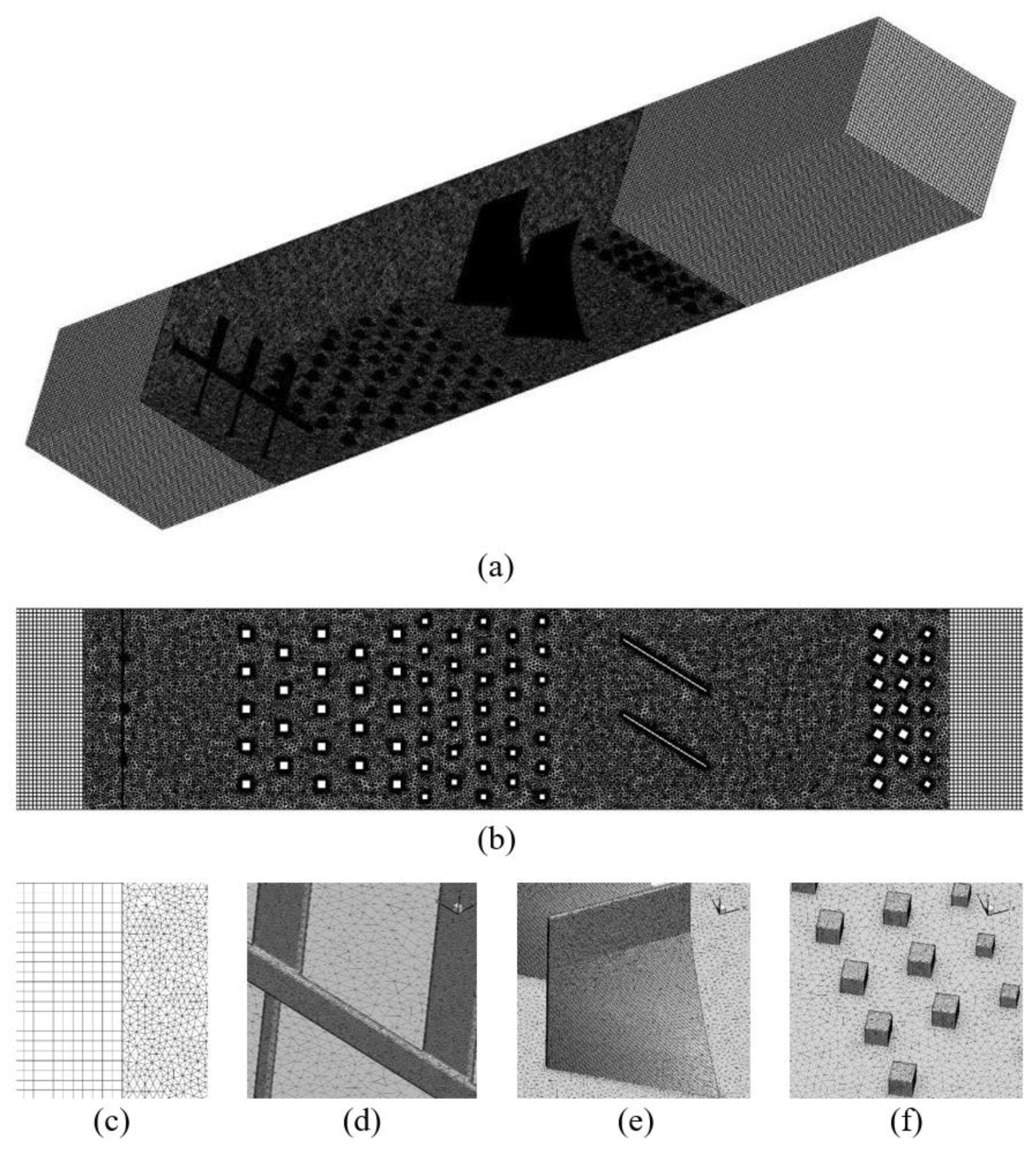
The LES technique was adopted herein to incorporate the ABL characteristics in the numerical wind tunnel. The validation work for grid independence and the LES turbulence model followed the process described in Section 4.1. Subsequently, conventional passive devices, including spires, fences, and ground roughness elements, were modeled in the numerical wind tunnel to generate the ABL characteristics of the flow, while guide vanes were implemented based on the optimal configuration obtained in Section 4.2, i.e., d v a n e , w a l l = 750 mm, d v a n e , v a n e = 700 mm, and d v a n e , m o d e l = 4 m. Based on the longitudinal wind speed profile in Figure 13a that corresponds to such a configuration of vanes, the conventional passive devices were carefully set up in the numerical wind tunnel so that the speed profile could be further modified into a power-law form, as expressed in Equation (4). Figure 14 depicts the mesh details in the computational domain as well as the setup of all passive devices. The simulation duration is 42.8 s in total with a time step of 0.001 s, and the results obtained within the first 6.5 s were excluded to avoid the unsteady flow generated at the start of the process.
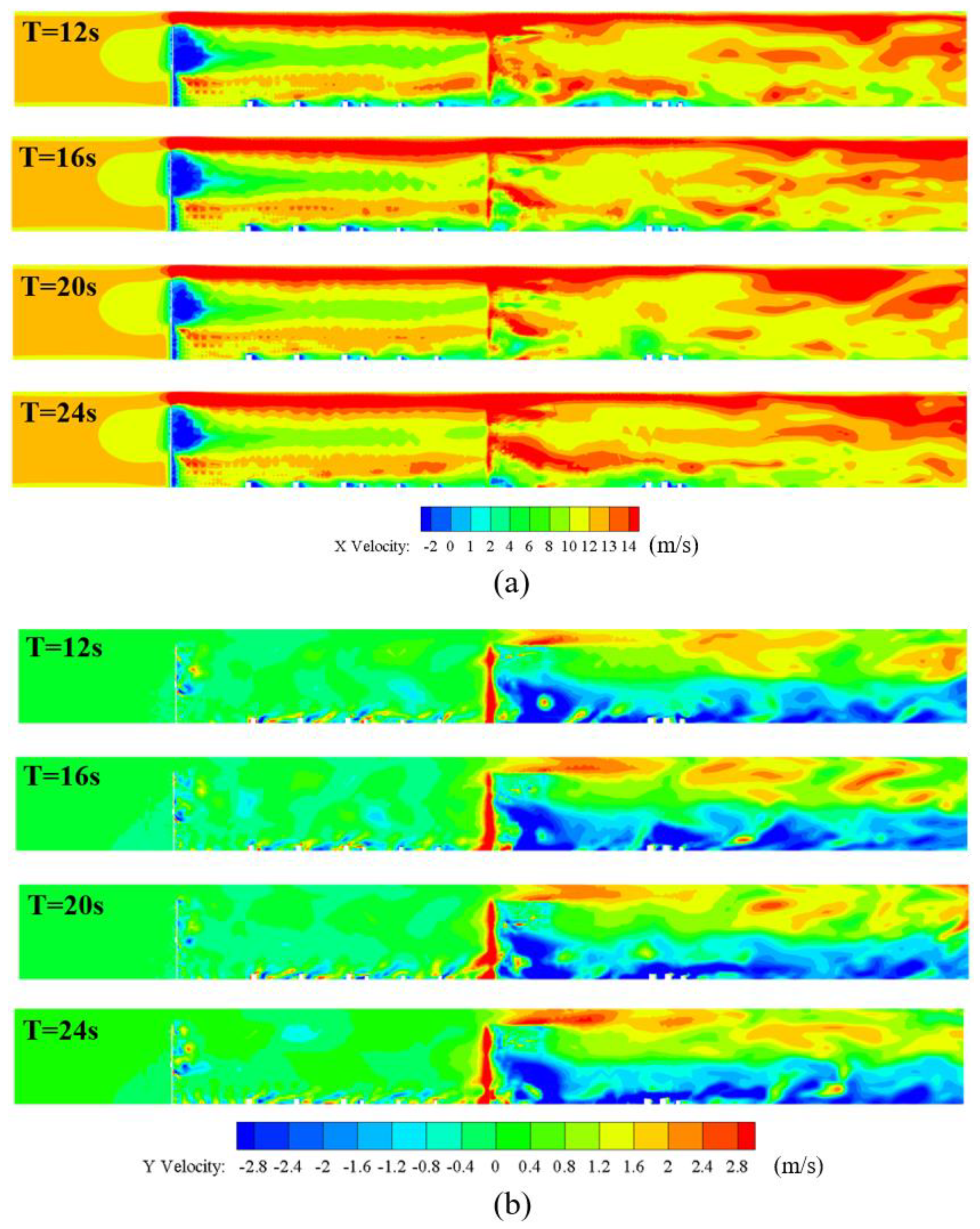
To evaluate the performance of the numerical wind tunnel setup, Figure 15a,b illustrate the time variations in the instantaneous longitudinal and lateral wind speeds, respectively, over time at the central plane of the wind tunnel. Figure 15a shows that, due to the employment of passive devices for generating ABL winds, the longitudinal wind speed increased with height as desired. On the other hand, the lateral wind speed increased significantly in the downstream region of the guide vanes, as shown in Figure 15b. All flow fields captured at time instances T = 12, 16, 20, and 24 s presented high similarity, suggesting that the TWF was stable during such a time period.
Figure 16 plots the profiles of TWF at the center of the model test region. As shown in Figure 16a, the longitudinal wind speed and turbulence intensity follow the power law expressed by Equation (4) and Equation (5), respectively. This indicates that the objective of incorporating ABL characteristics is generally satisfied. On the other hand, Figure 16b shows that the twist angle profile is generally in good agreement with the target profile (i.e., the Ekman spiral model) at heights above 0.4 m. However, the twist angles below 0.4 m were considerably lower than the desired values, which is believed to be attributed to the attenuation over distance and will be further improved at the subsequent closeout stage.

5. Closeout Stage

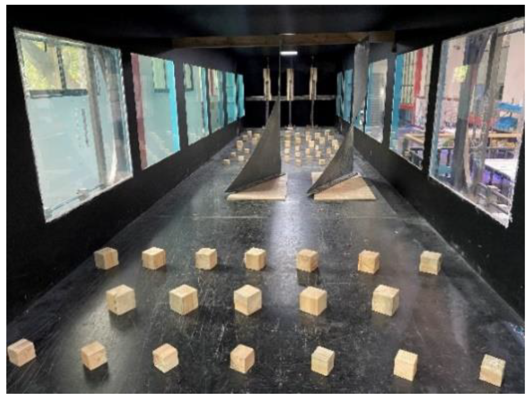
Following the setup in the numerical wind tunnel as discussed in Section 4.3, the passive devices, including the vane system, were implemented in the actual wind tunnel as shown in Figure 17. Considering that the twist angle values at heights below 0.4 m were lower than the desired values, the guide vanes were moved closer to the model test region by 200 mm (i.e., d v a n e , m o d e l = 3.8 m) to alleviate the attenuation of twist characteristics. Table 2 summarizes the final experimental setup of the guide vanes at the closeout stage, i.e., the optimal guide vane setup obtained following the procedure framework proposed by this study. It is noteworthy that the experimental setups are highly dependent on the specifications of the wind tunnel, and, therefore, modifications of setup parameters may be needed when generating the TWF wind profiles in another wind tunnel.
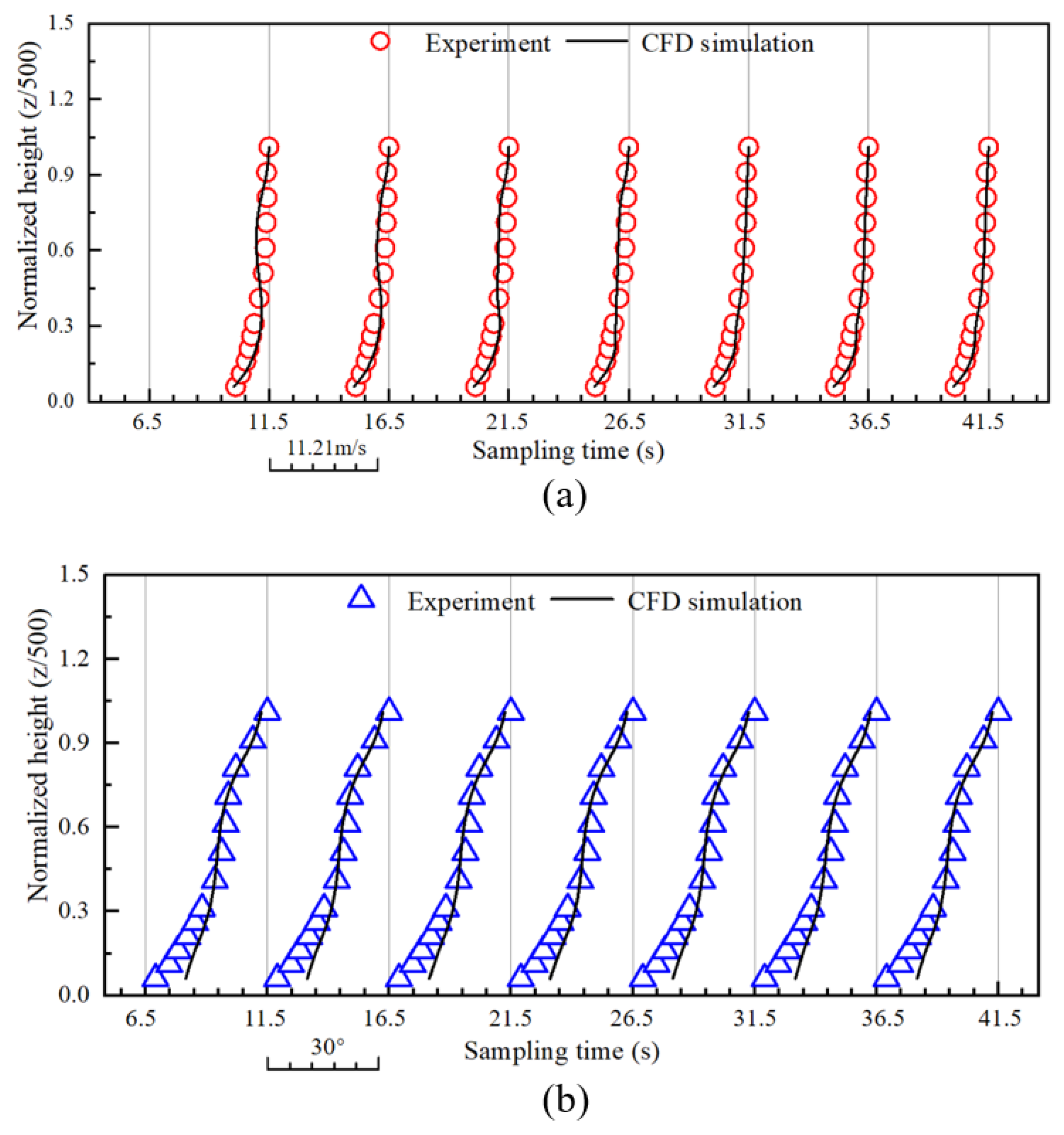
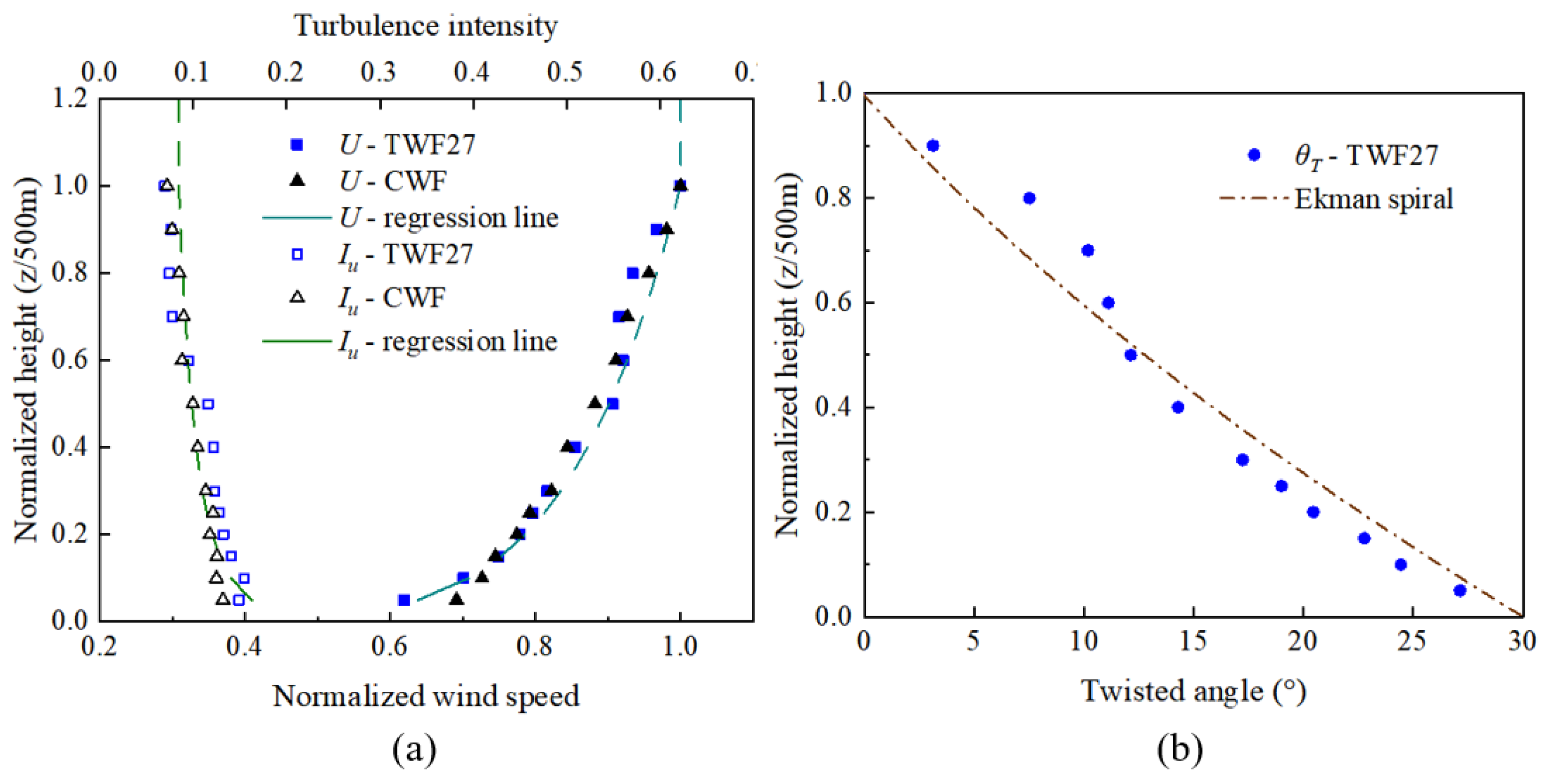
Figure 18 presents the variations in the profiles of longitudinal wind speed and turbulence intensity obtained from the numerical wind tunnel over time, indicating that the flow simulated by the LES technique became steady within approximately 30 s. In addition, the profiles obtained from the actual wind tunnel tests are also plotted in Figure 18 for comparison purposes, and good agreement between the LES-simulated profiles and the measured ones can be readily observed. Such agreement suggests that the numerical wind tunnel can serve as an efficient and accurate approach to provide useful reference to the actual wind tunnel tests.
Figure 19 plots the profiles of longitudinal speed, turbulence intensity, and twist angle of the TWF. As presented in Figure 19a, both profiles follow the power law expressed by Equations (4) and (5) with an exponent of 0.12 and −0.22, respectively. Furthermore, the profiles of conventional ABL wind flow (CWF) without twist were also generated in the wind tunnel as a reference. Good agreement can be readily observed between the profiles of the TWF and those of the CWF, indicating that the experimental setup for the TWF has produced ABL characteristics that are satisfactory. On the other hand, Figure 19b shows that the maximum twist angle of the TWF reached 27°, which is only slightly below the 30° set for the Ekman spiral model, and the measured twist angles well match the target values with a maximum discrepancy below 3°. Furthermore, Figure 20 shows that the power spectral densities of the longitudinal and lateral wind speeds, obtained by the Welch and Yule–Walker methods, are in good agreement with the Von Karman spectrum model. These results indicate that the guide vane system, configured following the procedural framework proposed in this study, has generated the desired TWF with satisfying accuracy.

6. Concluding Remarks

This paper has presented a procedural framework to achieve the optimal experimental setup for the generation of TWF in a wind tunnel based on CFD simulation results. Following the proposed procedures, the optimal configuration of the passive devices, especially the design of the guide vane system, to generate the desired TWF can be efficiently obtained by CFD simulation results in a numerical wind tunnel, enabling informed decisions for the final experimental setup in the actual wind tunnel. Several concluding remarks are drawn as follows:
(1)
The numerical wind tunnel established using the RANS and LES techniques can serve as an effective tool to examine the rationality of the experimental setup. The RNG k-ε model for RANS delivered the best predictions of wind speed in a numerical wind tunnel, according to the comparison with the results from the actual wind tunnel. The LES model, the more computationally efficient approach, was also able to numerically simulate the wind field with satisfying accuracy.
(2)
Based on the numerical simulation results, the mechanism of a guide vane system in a TWF simulation has been discussed in detail. Three parameters governing the positions of the vanes have been emphasized in this study and need to be considered carefully. First, d v a n e , w a l l is required to be sufficiently large so that the flow can travel through the gap and form a desired high-speed area in the downstream region. Second, d v a n e , v a n e needs to be sufficiently low to shorten the unfavorable length of the low-speed area and to prevent this area from reaching the model test region. Third, d v a n e , m o d e l must strike a balance so that it is not too large to cause the attenuation of the twist characteristics and not too small to allow the low-speed region to reach the model test region.
(3)
The numerical wind tunnel testing has demonstrated its applicability in providing valuable information for optimizing the experimental setups in the actual wind tunnel. By implementing passive devices in the actual wind tunnel following the setup used in its numerical counterpart, the desired TWF profiles have been generated with satisfying accuracy, i.e., the profiles of wind speed and turbulence intensity follow the power-law model for typical ABL winds, while the twist angle profile follows the Ekman spiral model. These results underscore the importance of utilizing numerical simulations to aid in the design of experimental setups, especially for novel devices such as the guide vane system discussed in the present study.

Author Contributions

Conceptualization, Z.Y., X.L., Z.Z. and B.Y.; methodology, Z.Y., X.L. and Z.Z.; software, L.W.; investigation, L.W., X.L. and X.Z.; resources, B.Y.; writing—original draft preparation, L.W.; writing—review and editing, Z.Y. and X.L.; supervision, B.Y.; project administration, B.Y.; funding acquisition, B.Y. All authors have read and agreed to the published version of the manuscript.

Funding

This research was funded by the National Natural Science Foundation of China (No. 51878104 and No. 52278483), the Graduate Research and Innovation Foundation of Chongqing, China (CYB21028), and the 111 Project of China (B18062).

Institutional Review Board Statement

Not applicable.

Informed Consent Statement

Not applicable.

Data Availability Statement

The data presented in this study are available on request from the corresponding author. The data are not publicly available due to privacy.

Conflicts of Interest

The authors declare no conflicts of interest.

Nomenclature

U Longitudinal mean wind speed e r lim Preset error threshold
I u Longitudinal turbulence intensity e r W T , C F D Difference between the wind tunnel test results and the CFD simulation results
θ T Twist angle e r obj , CFD Difference between the objective TWF wind profile and the CFD simulation results
z Height above ground d v a n e , w a l l Distance from the leading edge of the leftmost guide vane to the side wall of the wind tunnel
θ vane Twist angle of guide vane d v a n e , v a n e Spacing between guide vanes
H vane Height of guide vane d v a n e , m o d e l Distance from the trailing edge of the guide vanes to the center of the model test region

References

  1. Mendenhall, B.R. A Statistical Study of Frictional Wind Veering in the Planetary Boundary Layer. Atmospheric Science Paper. Ph.D. Dissertation, Colorado State University, Fort Collins, CO, USA, 1967. [Google Scholar]
  2. Tamura, Y.; Iwatani, Y.; Hibi, K.; Suda, K.; Nakamura, O.; Maruyama, T.; Ishibashi, R. Profiles of mean wind speeds and vertical turbulence intensities measured at seashore and two inland sites using Doppler sodars. J. Wind Eng. Ind. Aerodyn. 2007, 95, 411–427. [Google Scholar] [CrossRef]
  3. Liu, Z.; Zheng, C.; Wu, Y.; Song, Y. Investigation on characteristics of thousandmeter height wind profiles at non-tropical cyclone prone areas based on field measurement. Build Environ. 2018, 130, 62–73. [Google Scholar] [CrossRef]
  4. He, Y.C.; Chan, P.W.; Li, Q.S. Observations of vertical wind profiles of tropical cyclones at coastal areas. J. Wind Eng. Ind. Aerodyn. 2016, 152, 1–14. [Google Scholar] [CrossRef]
  5. Shu, Z.R.; Li, Q.S.; He, Y.C.; Chan, P.W. Observational study of veering wind by Doppler wind profiler and surface weather station. J. Wind Eng. Ind. Aerodyn. 2018, 178, 18–25. [Google Scholar] [CrossRef]
  6. Peña, A.; Gryning, S.E.; Floors, R. The turning of the wind in the atmospheric boundary layer. J. Phys. Conf. Ser. 2014, 524, 012118. [Google Scholar] [CrossRef]
  7. Yan, B.; Li, Y.; Li, X.; Zhou, X.; Wei, M.; Yang, Q.; Zhou, X. Wind tunnel investigation of twisted wind effect on a typical super-tall building. Buildings 2022, 12, 2260. [Google Scholar] [CrossRef]
  8. Tse, K.T.; Weerasuriya, A.U.; Kwok, K.C.S. Simulation of twisted wind flows in a boundary layer wind tunnel for pedestrian-level wind tunnel tests. J. Wind Eng. Ind. Aerodyn. 2016, 159, 99–109. [Google Scholar] [CrossRef]
  9. Flay, R.G. A twisted flow wind tunnel for testing yacht sails. J. Wind. Eng. Ind. Aerodyn. 1996, 63, 171–182. [Google Scholar] [CrossRef]
  10. Viola, I.M.; Fossati, F. Downwind Sails Aerodynamic Analysis. In Proceedings of the 6th International Colloquium on Bluff Bodies Aerodynamics and Applications, Milano, Italy, 20–24 July 2008. [Google Scholar]
  11. Graf, K.; Müller, O. Photogrammetric investigation of the flying shape of spinnakers in a twisted flow wind tunnel. In Proceedings of the 19th Chesapeake Sailing Yacht Symposium, Annapolis, MD, USA, 20 March 2009. [Google Scholar]
  12. Weerasuriya, A.U.; Tse, K.T.; Zhang, X.L.; Li, S.W. A wind tunnel study of effects of twisted wind flows on the pedestrian-level wind field in an urban environment. Build Environ. 2018, 128, 225–235. [Google Scholar] [CrossRef]
  13. Zhou, L.; Tse, K.T.; Hu, G. Experimental investigation on the aerodynamic characteristics of a tall building subjected to twisted wind. J. Wind Eng. Ind. Aerodyn. 2022, 224, 104976. [Google Scholar] [CrossRef]
  14. Liu, Z.; Zheng, C.; Wu, Y.; Flay, R.G.J.; Zhang, K. Wind tunnel simulation of wind flows with the characteristics of thousand-meter high ABL. Build Environ. 2019, 152, 74–86. [Google Scholar] [CrossRef]
  15. Yan, B.W.; Li, Q.S.; He, Y.C.; Chan, P.W. RANS simulation of neutral atmospheric boundary layer flows over complex terrain by proper imposition of boundary conditions and modification on the k-ε model. Environ. Fluid Mech. 2016, 16, 1–23. [Google Scholar] [CrossRef]
  16. Weerasuriya, A.U.; Hu, Z.Z.; Zhang, X.L.; Tse, K.T.; Li, S.; Chan, P.W. New inflow boundary conditions for modeling twisted wind profiles in CFD simulation for evaluating the pedestrian-level wind field near an isolated building. Build. Environ. 2018, 132, 303–318. [Google Scholar] [CrossRef] [PubMed]
  17. Feng, C.; Gu, M.; Zheng, D. Numerical simulation of wind effects on super highrise buildings considering wind veering with height based on CFD. J. Fluids Struct. 2019, 91, 102715. [Google Scholar] [CrossRef]
  18. Lu, B.; Li, Q.S. Large eddy simulation of the atmospheric boundary layer to investigate the Coriolis effect on wind and turbulence characteristics over different terrains. J. Wind Eng. Ind. Aerodyn. 2022, 220, 104845. [Google Scholar] [CrossRef]
  19. Aly, A.M.; Bitsuamlak, G. Aerodynamics of ground-mounted solar panels: Test model scale effects. J. Wind. Eng. Ind. Aerodyn. 2013, 123, 250–260. [Google Scholar] [CrossRef]
  20. Phuc, P.V.; Nozu, T.; Kikuchi, H.; Hibi, K.; Tamura, Y. Wind pressure distributions on buildings using the coherent structure Smagorinsky model for LES. J. Comput. 2018, 6, 32. [Google Scholar] [CrossRef]
  21. Le, V.; Caracoglia, L. Generation and characterization of a non-stationary flow field in a small-scale wind tunnel using a multi-blade flow device. J. Wind. Eng. Ind. Aerodyn. 2019, 186, 1–16. [Google Scholar] [CrossRef]
  22. Marks, F.D.; Dodge, P.; Sandin, C. WSR-88D observations of hurricane atmospheric boundary layer structure at landfall. In Proceedings of the 23d Conference on Hurricanes and Tropical Meteorology (American Meteorology Society), Dallas, TX, USA, 10–15 January 1999; pp. 1051–1054. [Google Scholar]
  23. Ekman, V.W. On the Influence of the Earth’s Rotation on Ocean Currents; Arkiv för Matematik, Astronomi Och Fysik; Almqvist & Wiksells Boktryckeri, A.-B.: Uppsala, Sweden, 1905; Band 2; pp. 1–52. [Google Scholar]
  24. Smagorinsky, J. General circulation experiments with the primitive equations. Mon. Weather. Rev. 1963, 91, 99–164. [Google Scholar] [CrossRef]
  25. Launder, B.E.; Spalding, D.B. Lectures in Mathematical Model of Turbulence; Academic Press: London, UK, 1972. [Google Scholar]
  26. Yakhot, V.; Orszag, S.A. Renormalization group analysis of turbulence: Basic theory. J. Sci. Comput. 1986, 1, 3–51. [Google Scholar] [CrossRef]
  27. Shih, T.H.; Liou, W.W.; Shabbir, A.; Yang, Z.; Jiang, Z. A new k-ε eddy viscosity model eynolds reynolds number turbulent flows. Comput. Fluids 1995, 24, 227–238. [Google Scholar] [CrossRef]
  28. Wilcox, D.C. Reassessment of the scale-determining equation for advanced turbulence models. AIAA J. 1988, 26, 1299. [Google Scholar] [CrossRef]
  29. Menter, F.R. Two-equation eddy-viscosity turbulence models for engineering applications. AIAA J. 1994, 32, 1598–1605. [Google Scholar] [CrossRef]
  30. Roache, P.J.; Ghia, K.N.; White, F.M. Editorial policy statement on the control of numerical accuracy. J. Fluids Eng. 1986, 108, 2. [Google Scholar] [CrossRef]
Figure 1. Procedural framework for CFD-aided wind tunnel simulation of twisted wind flow.
Applsci 14 00988 g001
Figure 2. Comparison of common twist angle curve models.
Applsci 14 00988 g002
Figure 3. Dimensions of spires and ground roughness elements.
Applsci 14 00988 g003
Figure 4. Guide vanes for wind tunnel simulation of twisted wind flow.
Applsci 14 00988 g004
Figure 5. Dimensions of guide vanes: (a) front view; (b) top view.
Applsci 14 00988 g005
Figure 6. Positions of guide vanes and measurement points: (a) plan view; (b) side view.
Applsci 14 00988 g006
Figure 7. Twist angle profiles measured within model test region.
Applsci 14 00988 g007
Figure 8. Basic information of numerical wind tunnel.
Applsci 14 00988 g008
Figure 9. Mesh details of numerical wind tunnel for validation case.
Applsci 14 00988 g009
Figure 10. Comparisons of mean wind speeds obtained by CFD with different RANS turbulence models and by actual wind tunnel tests.
Applsci 14 00988 g010
Figure 11. Distribution of lateral mean wind speed at z = 0.3 m: (a) d v a n e , w a l l = 450 mm; (b) d v a n e , w a l l = 600 mm; (c) d v a n e , w a l l = 750 mm.
Applsci 14 00988 g011
Figure 12. Distribution of lateral mean wind speed at z = 0.3 m: (a) d v a n e , v a n e = 700 mm; (b) d v a n e , v a n e = 800 mm; (c) d v a n e , v a n e = 900 mm; (d) d v a n e , v a n e = 1000 mm.
Applsci 14 00988 g012
Figure 13. Wind profiles at different locations on the X-axis: (a) longitudinal mean wind speed; (b) longitudinal turbulence intensity; (c) twist angle.
Applsci 14 00988 g013
Figure 14. Mesh details for optimal setup in numerical wind tunnel: (a) overview; (b) top view of test section; (c) connection of grid nodes; (d) close-up view of spires and fence; (e) close-up view of guide vanes; (f) close-up view of ground roughness elements.
Applsci 14 00988 g014
Figure 15. Time variations in the instantaneous wind speeds: (a) longitudinal speed; (b) lateral speed.
Applsci 14 00988 g015
Figure 16. Wind profiles obtained by optimal setup in numerical wind tunnel: (a) longitudinal mean wind speed and turbulence intensity; (b) twist angle.
Applsci 14 00988 g016
Figure 17. Final setup in actual wind tunnel.
Applsci 14 00988 g017
Figure 18. Variations in wind profiles at different locations on the X-axis: (a) longitudinal mean wind speed; (b) twist angle.
Applsci 14 00988 g018
Figure 19. Wind profiles obtained by final setup in actual wind tunnel: (a) longitudinal mean wind speed and turbulence intensity; (b) twist angle.
Applsci 14 00988 g019
Figure 20. Wind spectra of TWF at z = 1.0 m: (a) longitudinal speed; (b) lateral speed.
Applsci 14 00988 g020
Table 1. Grid convergence analysis.
Number of Grids Wind   Speed   I (m/s) p 1 I r ( i , i + 1 ) ICI ( i , i + 1 )
2.45 × 1068.701.250.00570.0021
4.24 × 1068.65
0.02650.0101
7.34 × 1068.42
Table 2. Summary of optimal experimental setup of guide vanes.
ParameterValue
No. of vanes2
θ vane z modelEkman spiral
θ vane 0 30°
θ vane 1
θ vane 1.5
H vane 1.5 m
d v a n e , w a l l 750 mm
d v a n e , v a n e 700 mm
d v a n e , m o d e l 3800 mm
Disclaimer/Publisher’s Note: The statements, opinions and data contained in all publications are solely those of the individual author(s) and contributor(s) and not of MDPI and/or the editor(s). MDPI and/or the editor(s) disclaim responsibility for any injury to people or property resulting from any ideas, methods, instructions or products referred to in the content.