
Computational Fluid Dynamics-Aided Simulation of Twisted Wind Flows in Boundary Layer Wind Tunnel

Abstract
:1. Introduction
2. Procedural Framework
2.1. Preparation Stage
2.2. Development Stage
2.3. Closeout Stage
3. Preparation Stage
3.1. Target Wind Profiles
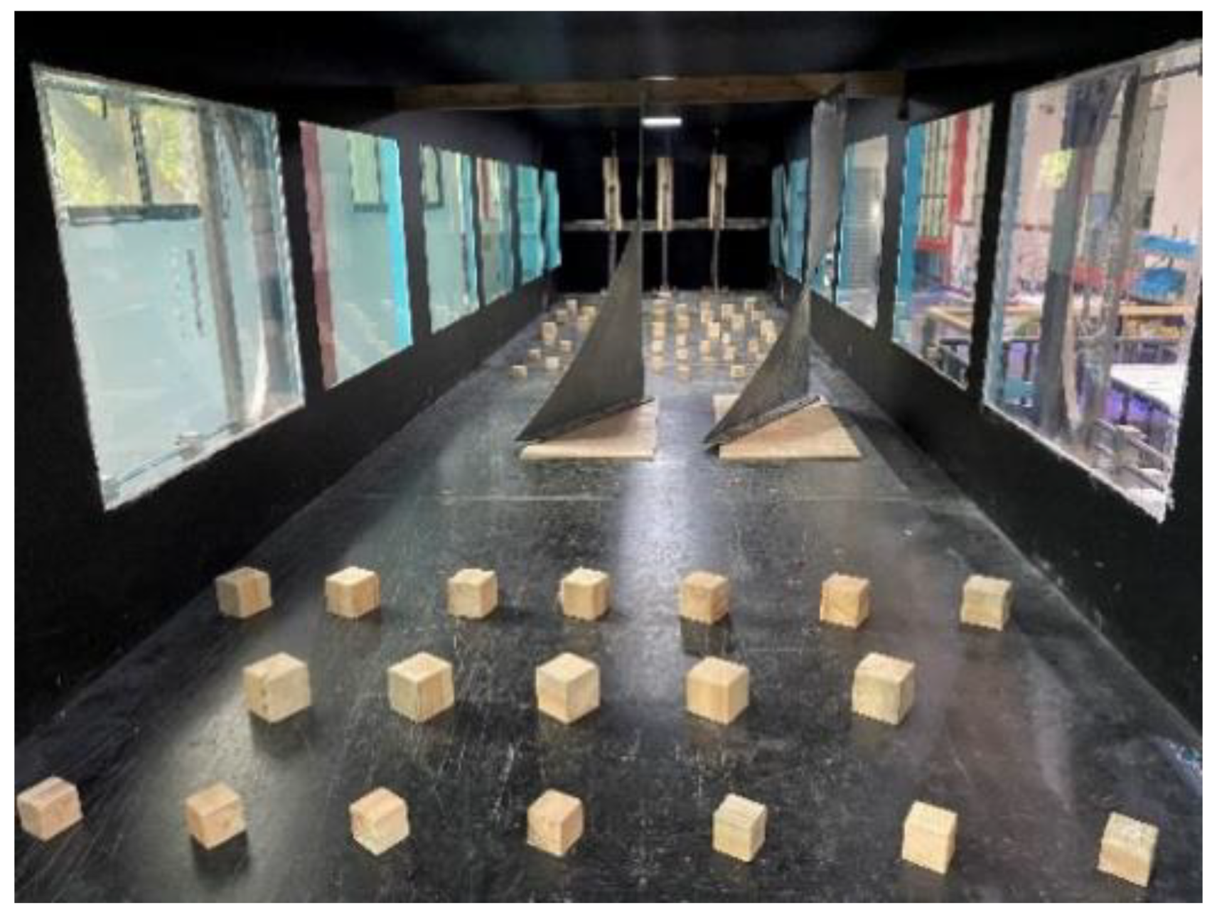
3.2. Wind Tunnel Setup
4. Development Stage
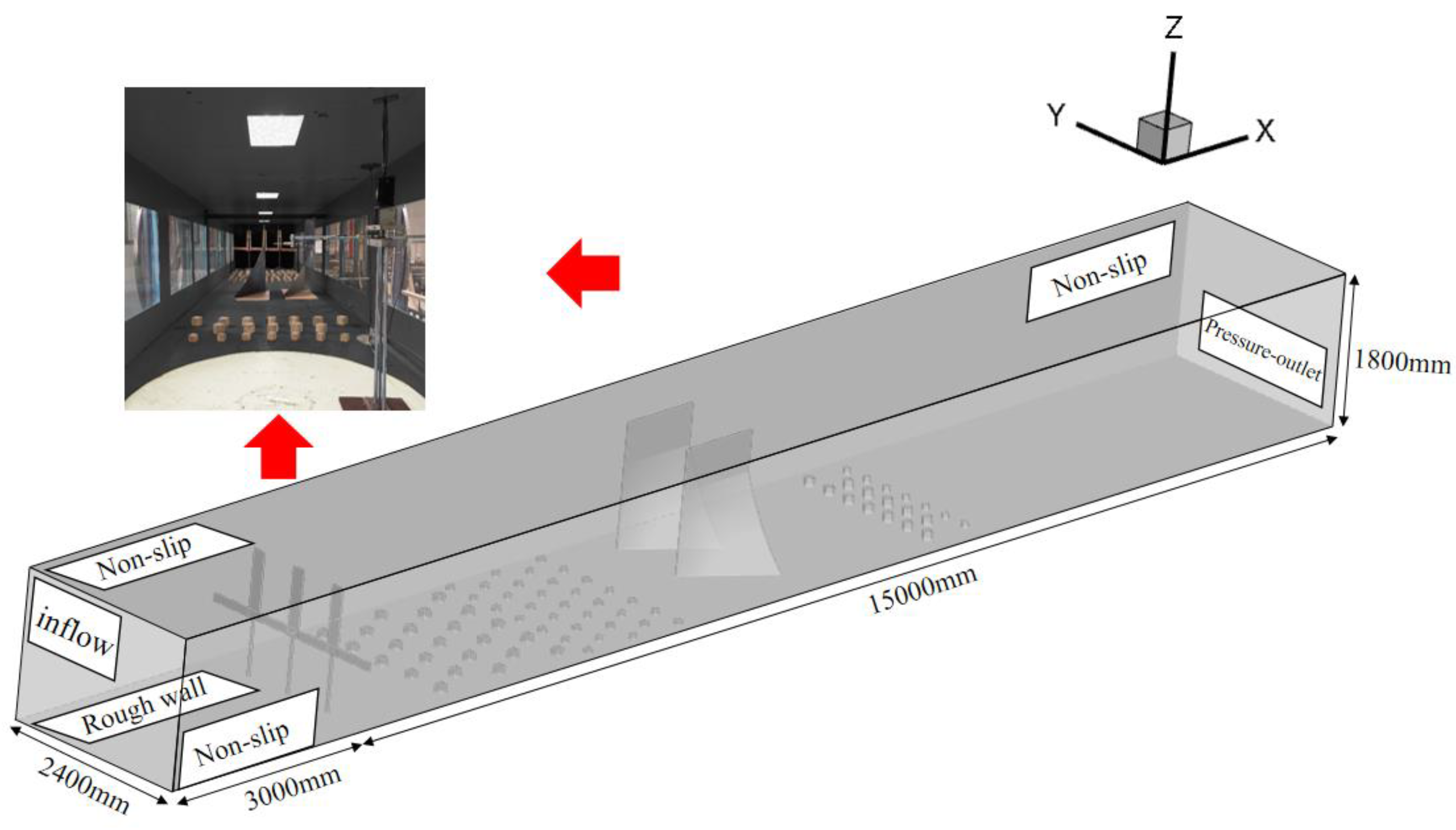
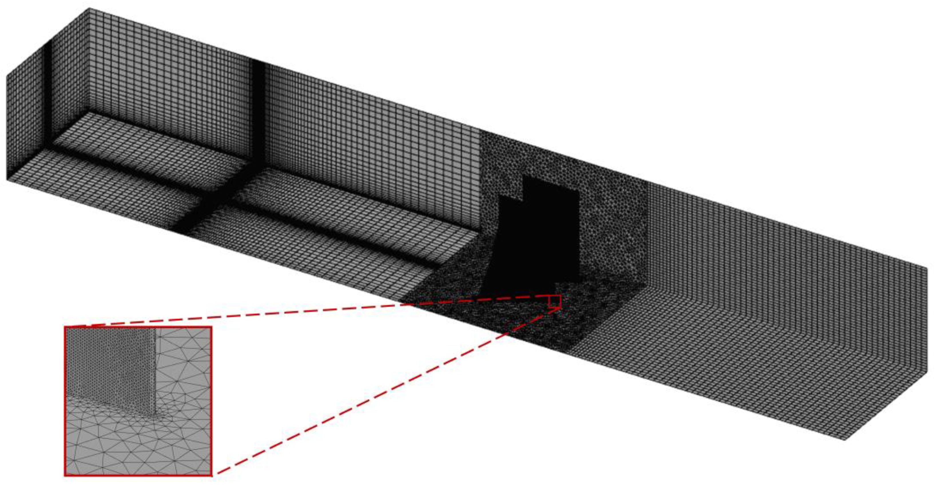
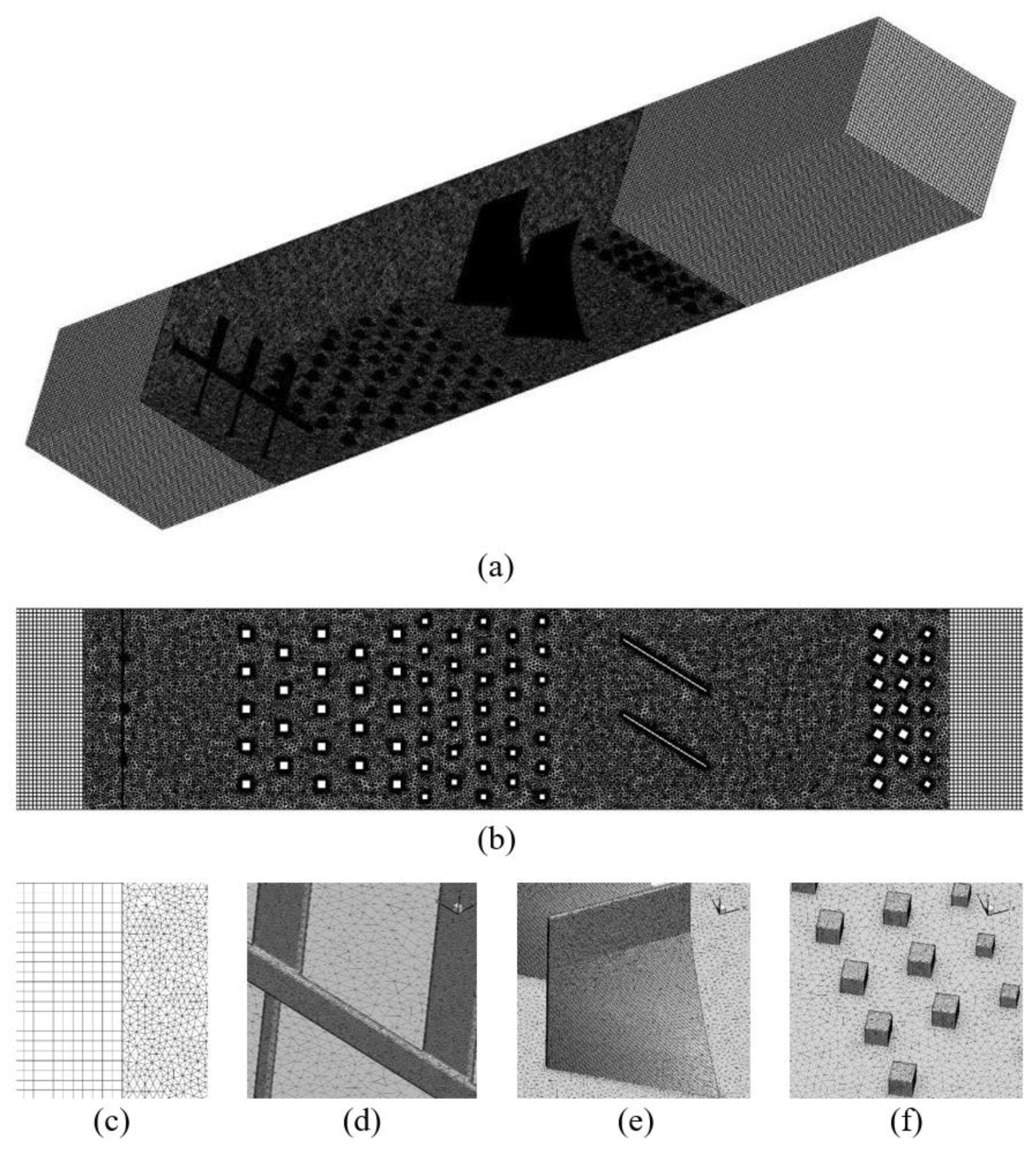
4.1. Establishment of Numerical Wind Tunnel
4.1.1. CFD Setup for Numerical Wind Tunnel
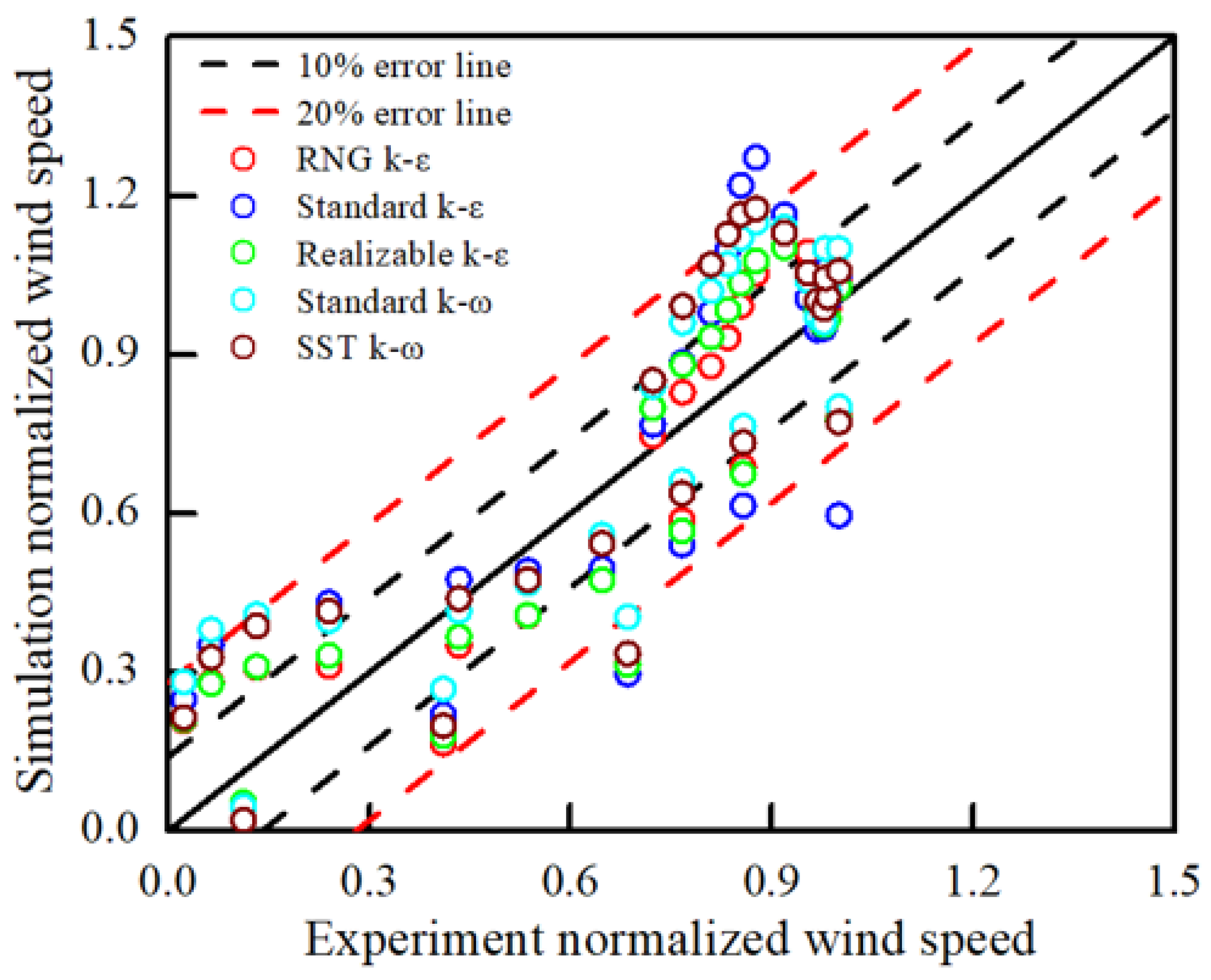
4.1.2. Validation of CFD Setup
4.2. Optimization of Guide Vane Configuration
4.2.1. Distance from Side Wall
4.2.2. Spacing between Guide Vanes
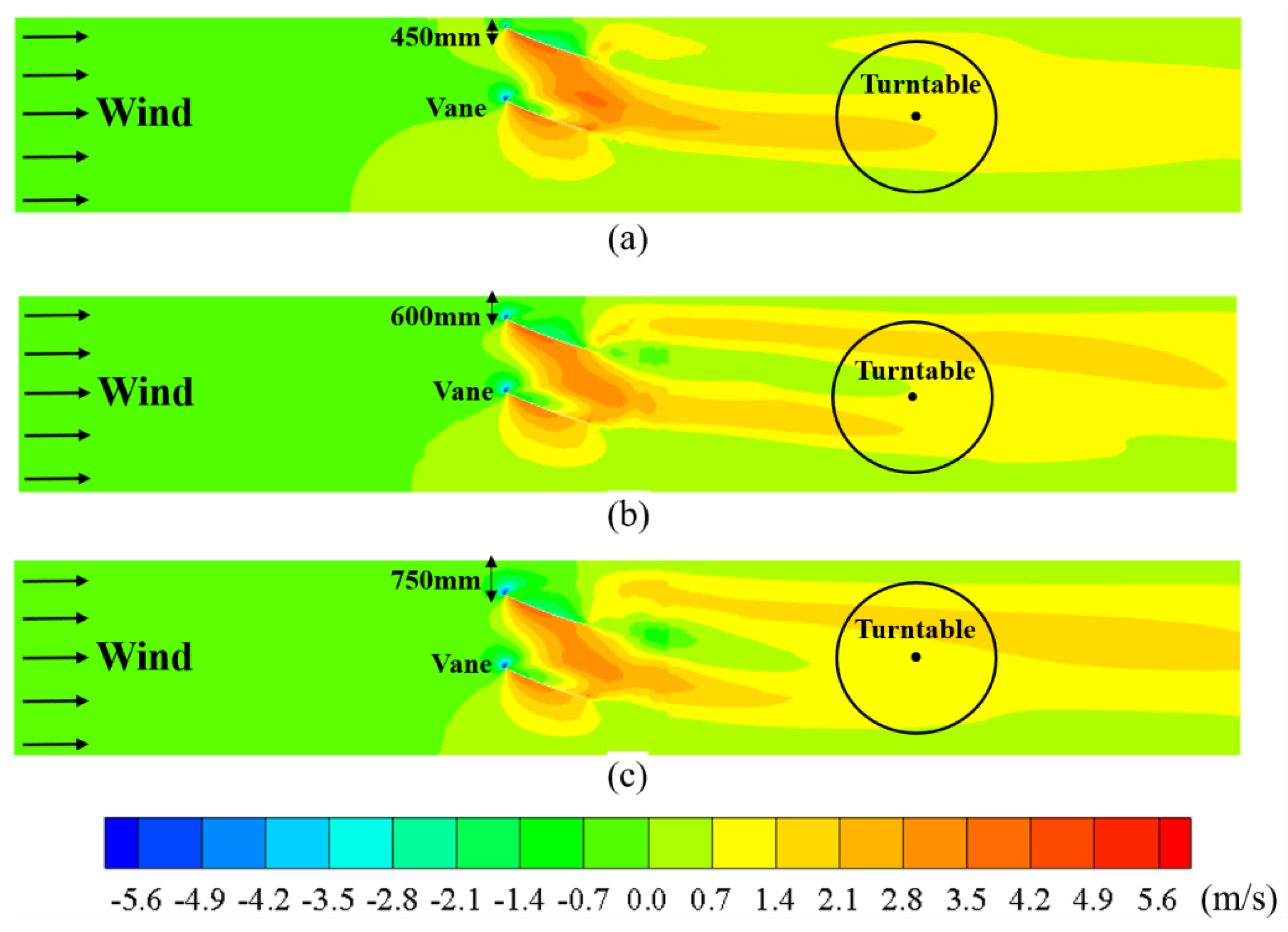
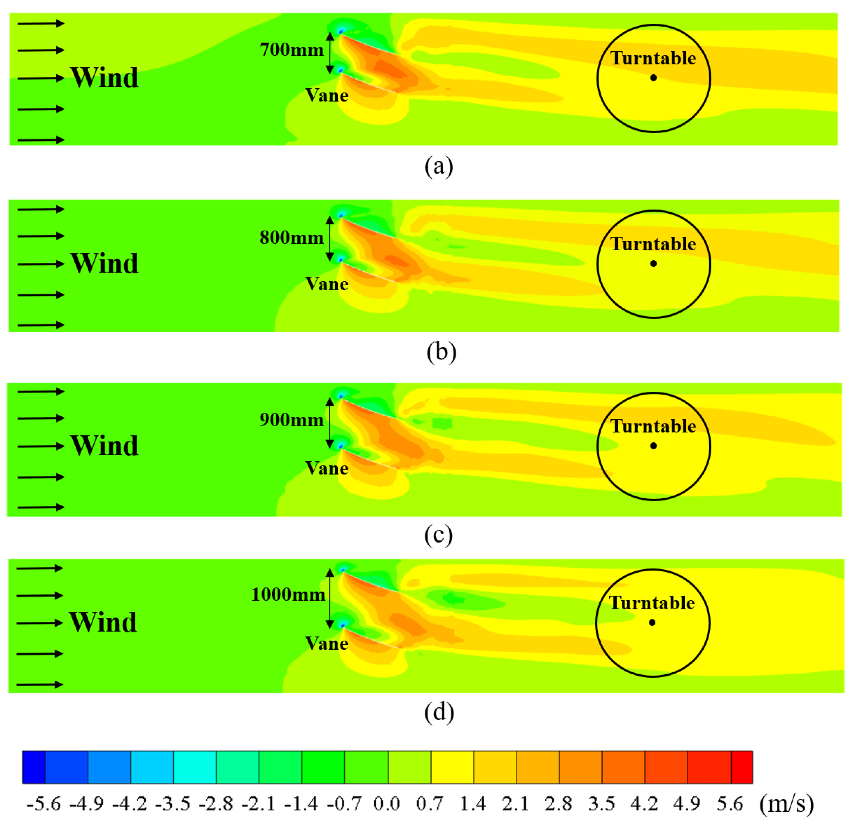
4.2.3. Distance between Trailing Edge of Guide Vane and Center of Turntable
4.3. Incorporation of ABL Characteristics
5. Closeout Stage
6. Concluding Remarks
- (1)
- The numerical wind tunnel established using the RANS and LES techniques can serve as an effective tool to examine the rationality of the experimental setup. The RNG k-ε model for RANS delivered the best predictions of wind speed in a numerical wind tunnel, according to the comparison with the results from the actual wind tunnel. The LES model, the more computationally efficient approach, was also able to numerically simulate the wind field with satisfying accuracy.
- (2)
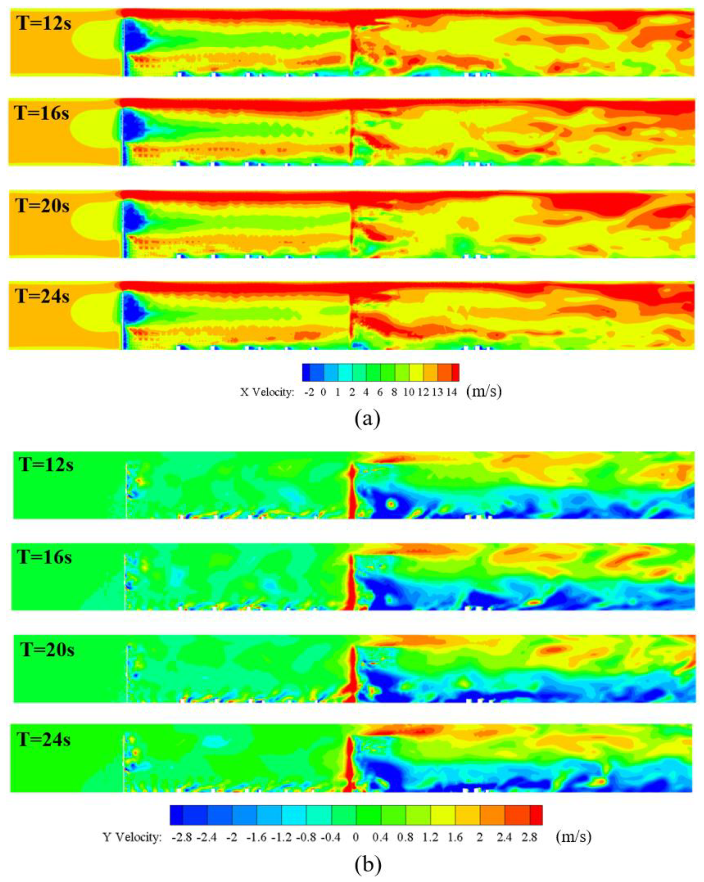
- Based on the numerical simulation results, the mechanism of a guide vane system in a TWF simulation has been discussed in detail. Three parameters governing the positions of the vanes have been emphasized in this study and need to be considered carefully. First, is required to be sufficiently large so that the flow can travel through the gap and form a desired high-speed area in the downstream region. Second, needs to be sufficiently low to shorten the unfavorable length of the low-speed area and to prevent this area from reaching the model test region. Third, must strike a balance so that it is not too large to cause the attenuation of the twist characteristics and not too small to allow the low-speed region to reach the model test region.
- (3)
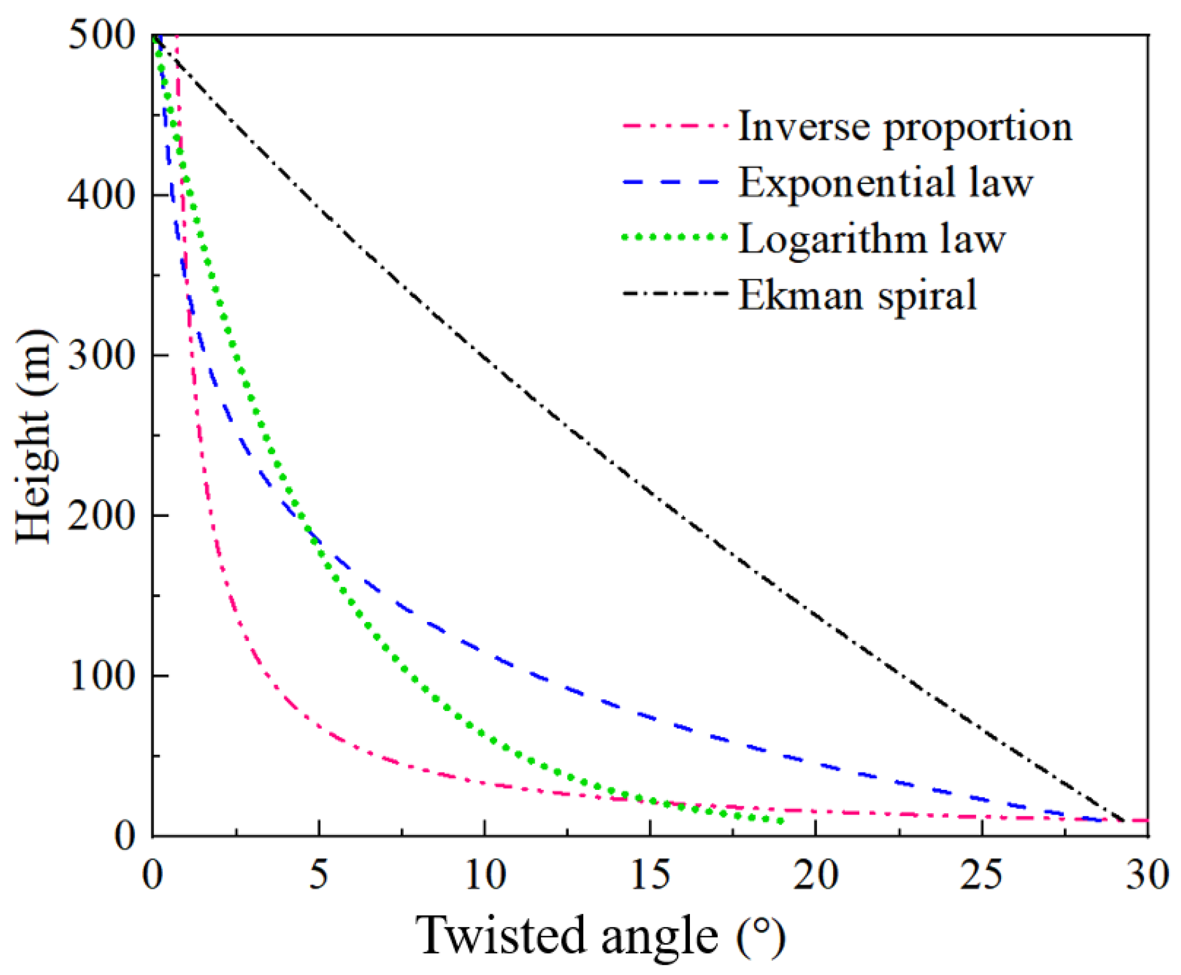
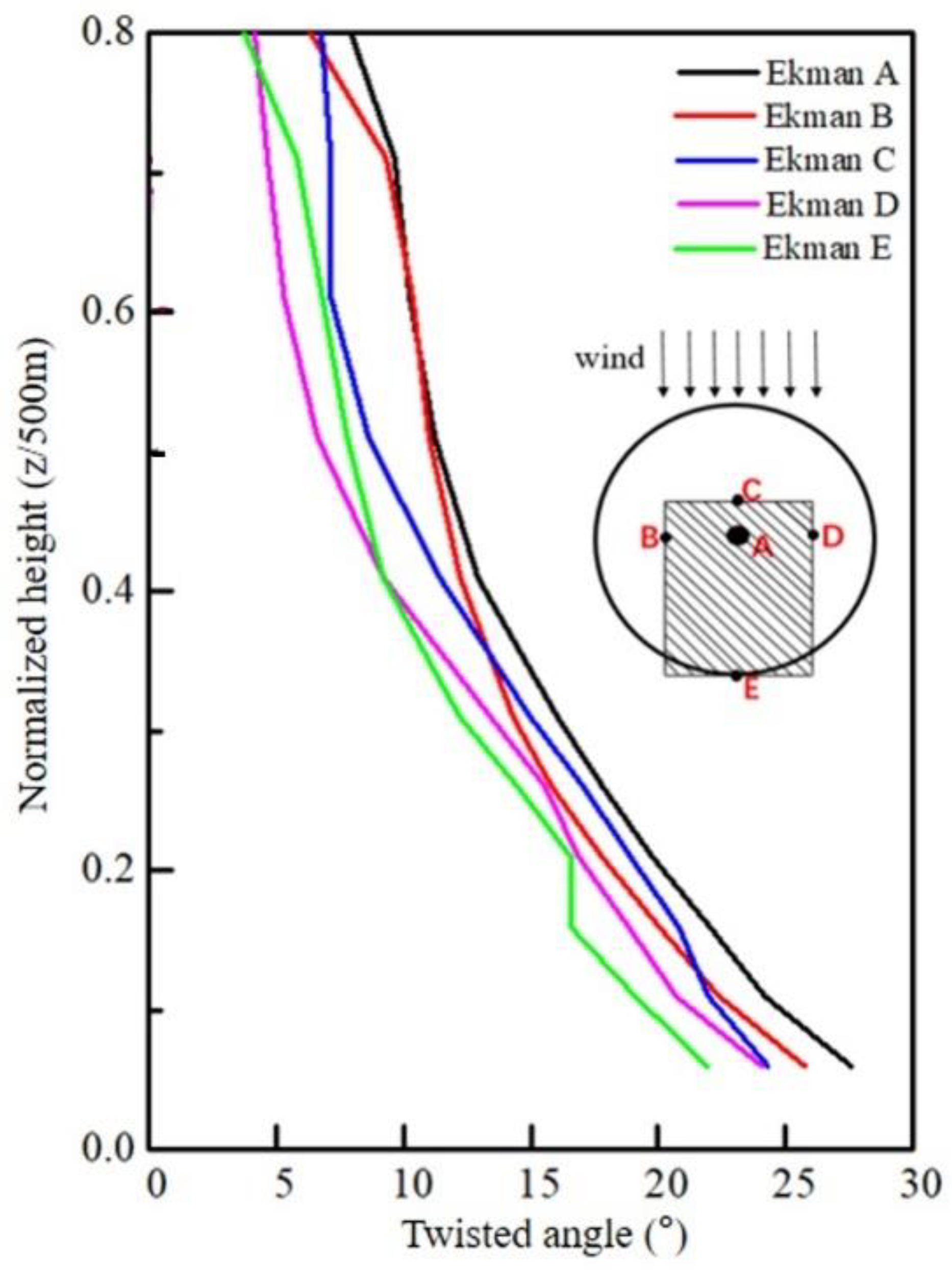
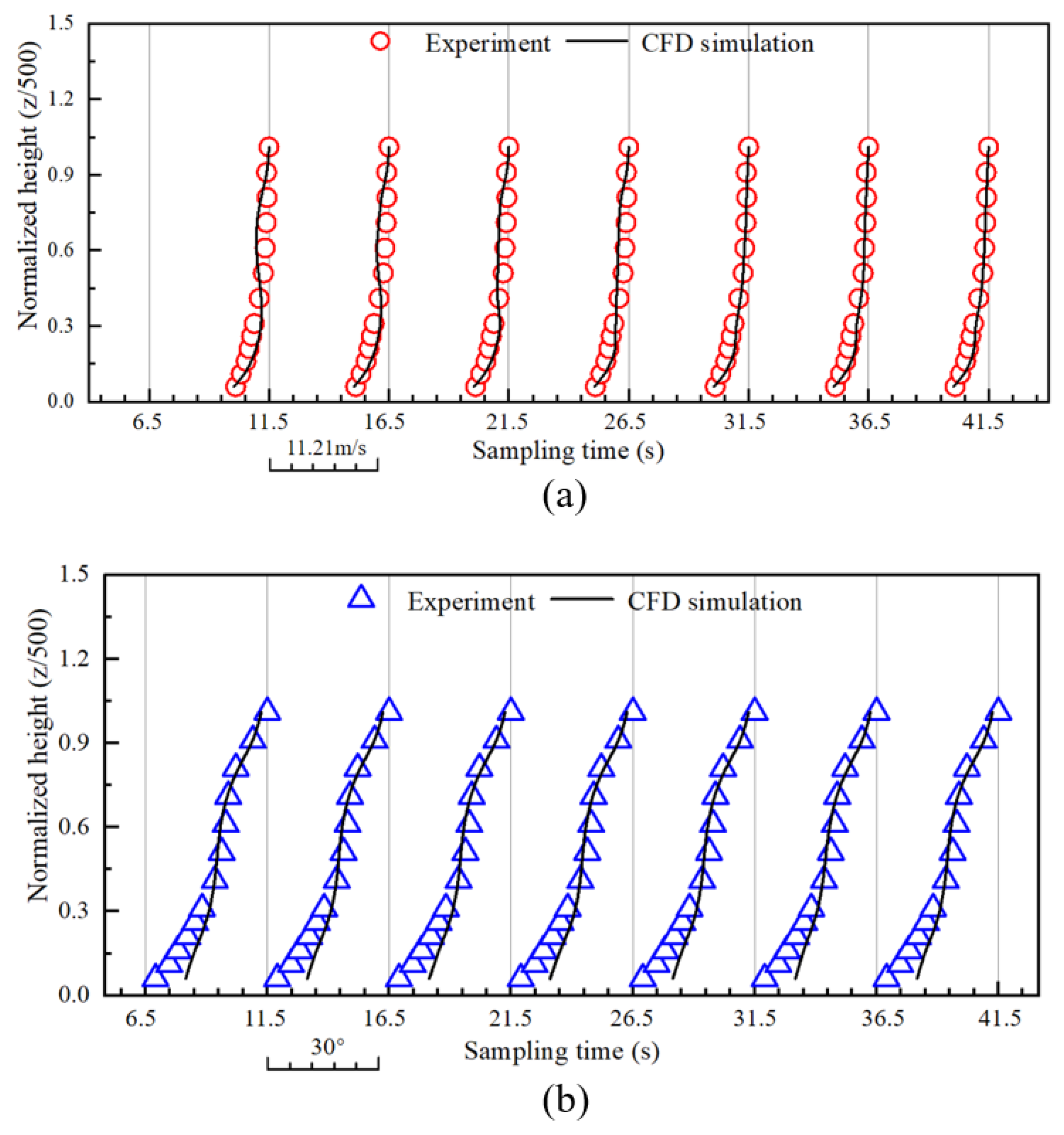
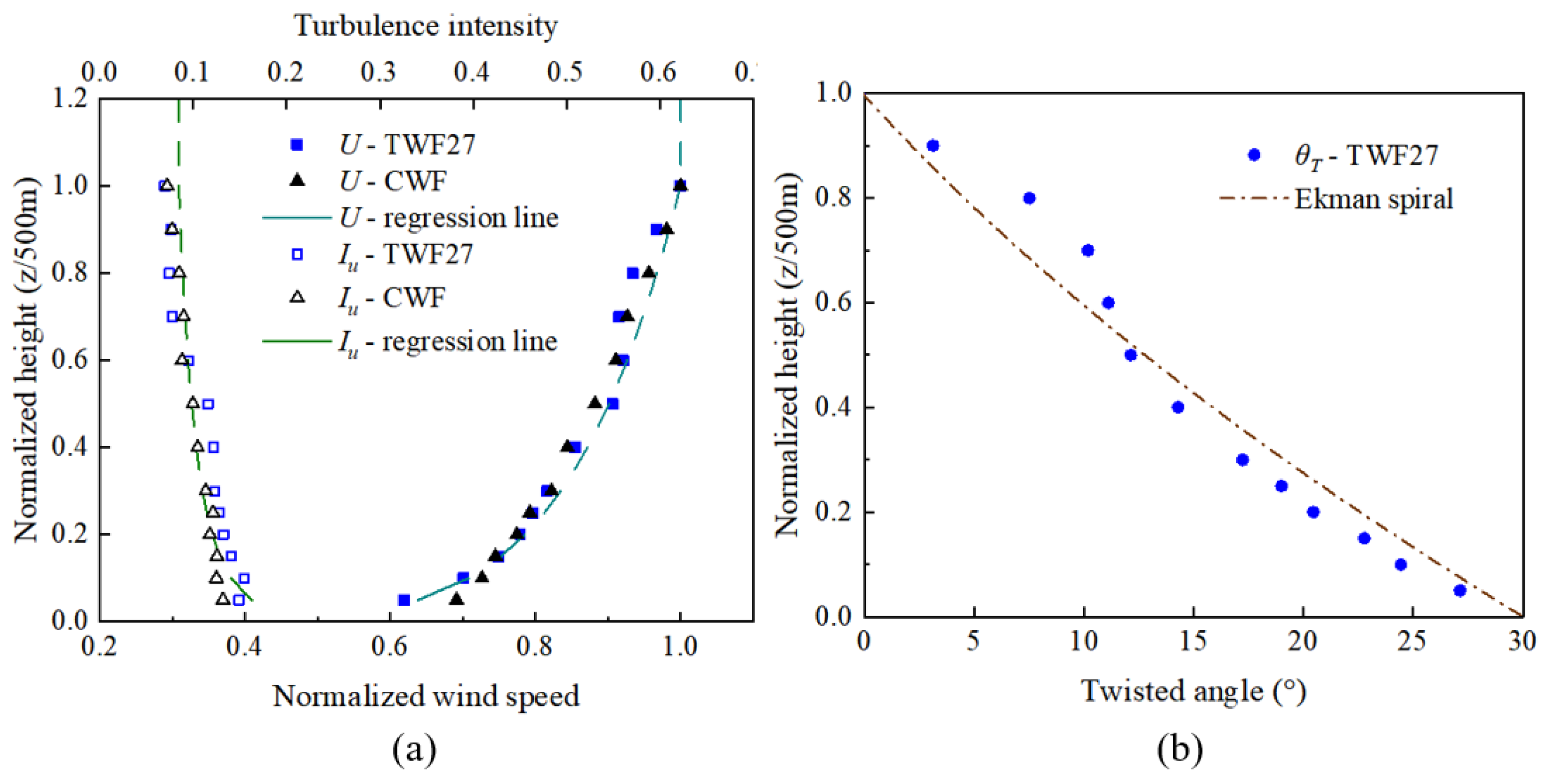
- The numerical wind tunnel testing has demonstrated its applicability in providing valuable information for optimizing the experimental setups in the actual wind tunnel. By implementing passive devices in the actual wind tunnel following the setup used in its numerical counterpart, the desired TWF profiles have been generated with satisfying accuracy, i.e., the profiles of wind speed and turbulence intensity follow the power-law model for typical ABL winds, while the twist angle profile follows the Ekman spiral model. These results underscore the importance of utilizing numerical simulations to aid in the design of experimental setups, especially for novel devices such as the guide vane system discussed in the present study.
Author Contributions
Funding
Institutional Review Board Statement
Informed Consent Statement
Data Availability Statement
Conflicts of Interest
Nomenclature
| Longitudinal mean wind speed | Preset error threshold | ||
| Longitudinal turbulence intensity | Difference between the wind tunnel test results and the CFD simulation results | ||
| Twist angle | Difference between the objective TWF wind profile and the CFD simulation results | ||
| Height above ground | Distance from the leading edge of the leftmost guide vane to the side wall of the wind tunnel | ||
| Twist angle of guide vane | Spacing between guide vanes | ||
| Height of guide vane | Distance from the trailing edge of the guide vanes to the center of the model test region |
References
- Mendenhall, B.R. A Statistical Study of Frictional Wind Veering in the Planetary Boundary Layer. Atmospheric Science Paper. Ph.D. Dissertation, Colorado State University, Fort Collins, CO, USA, 1967. [Google Scholar]
- Tamura, Y.; Iwatani, Y.; Hibi, K.; Suda, K.; Nakamura, O.; Maruyama, T.; Ishibashi, R. Profiles of mean wind speeds and vertical turbulence intensities measured at seashore and two inland sites using Doppler sodars. J. Wind Eng. Ind. Aerodyn. 2007, 95, 411–427. [Google Scholar] [CrossRef]
- Liu, Z.; Zheng, C.; Wu, Y.; Song, Y. Investigation on characteristics of thousandmeter height wind profiles at non-tropical cyclone prone areas based on field measurement. Build Environ. 2018, 130, 62–73. [Google Scholar] [CrossRef]
- He, Y.C.; Chan, P.W.; Li, Q.S. Observations of vertical wind profiles of tropical cyclones at coastal areas. J. Wind Eng. Ind. Aerodyn. 2016, 152, 1–14. [Google Scholar] [CrossRef]
- Shu, Z.R.; Li, Q.S.; He, Y.C.; Chan, P.W. Observational study of veering wind by Doppler wind profiler and surface weather station. J. Wind Eng. Ind. Aerodyn. 2018, 178, 18–25. [Google Scholar] [CrossRef]
- Peña, A.; Gryning, S.E.; Floors, R. The turning of the wind in the atmospheric boundary layer. J. Phys. Conf. Ser. 2014, 524, 012118. [Google Scholar] [CrossRef]
- Yan, B.; Li, Y.; Li, X.; Zhou, X.; Wei, M.; Yang, Q.; Zhou, X. Wind tunnel investigation of twisted wind effect on a typical super-tall building. Buildings 2022, 12, 2260. [Google Scholar] [CrossRef]
- Tse, K.T.; Weerasuriya, A.U.; Kwok, K.C.S. Simulation of twisted wind flows in a boundary layer wind tunnel for pedestrian-level wind tunnel tests. J. Wind Eng. Ind. Aerodyn. 2016, 159, 99–109. [Google Scholar] [CrossRef]
- Flay, R.G. A twisted flow wind tunnel for testing yacht sails. J. Wind. Eng. Ind. Aerodyn. 1996, 63, 171–182. [Google Scholar] [CrossRef]
- Viola, I.M.; Fossati, F. Downwind Sails Aerodynamic Analysis. In Proceedings of the 6th International Colloquium on Bluff Bodies Aerodynamics and Applications, Milano, Italy, 20–24 July 2008. [Google Scholar]
- Graf, K.; Müller, O. Photogrammetric investigation of the flying shape of spinnakers in a twisted flow wind tunnel. In Proceedings of the 19th Chesapeake Sailing Yacht Symposium, Annapolis, MD, USA, 20 March 2009. [Google Scholar]
- Weerasuriya, A.U.; Tse, K.T.; Zhang, X.L.; Li, S.W. A wind tunnel study of effects of twisted wind flows on the pedestrian-level wind field in an urban environment. Build Environ. 2018, 128, 225–235. [Google Scholar] [CrossRef]
- Zhou, L.; Tse, K.T.; Hu, G. Experimental investigation on the aerodynamic characteristics of a tall building subjected to twisted wind. J. Wind Eng. Ind. Aerodyn. 2022, 224, 104976. [Google Scholar] [CrossRef]
- Liu, Z.; Zheng, C.; Wu, Y.; Flay, R.G.J.; Zhang, K. Wind tunnel simulation of wind flows with the characteristics of thousand-meter high ABL. Build Environ. 2019, 152, 74–86. [Google Scholar] [CrossRef]
- Yan, B.W.; Li, Q.S.; He, Y.C.; Chan, P.W. RANS simulation of neutral atmospheric boundary layer flows over complex terrain by proper imposition of boundary conditions and modification on the k-ε model. Environ. Fluid Mech. 2016, 16, 1–23. [Google Scholar] [CrossRef]
- Weerasuriya, A.U.; Hu, Z.Z.; Zhang, X.L.; Tse, K.T.; Li, S.; Chan, P.W. New inflow boundary conditions for modeling twisted wind profiles in CFD simulation for evaluating the pedestrian-level wind field near an isolated building. Build. Environ. 2018, 132, 303–318. [Google Scholar] [CrossRef] [PubMed]
- Feng, C.; Gu, M.; Zheng, D. Numerical simulation of wind effects on super highrise buildings considering wind veering with height based on CFD. J. Fluids Struct. 2019, 91, 102715. [Google Scholar] [CrossRef]
- Lu, B.; Li, Q.S. Large eddy simulation of the atmospheric boundary layer to investigate the Coriolis effect on wind and turbulence characteristics over different terrains. J. Wind Eng. Ind. Aerodyn. 2022, 220, 104845. [Google Scholar] [CrossRef]
- Aly, A.M.; Bitsuamlak, G. Aerodynamics of ground-mounted solar panels: Test model scale effects. J. Wind. Eng. Ind. Aerodyn. 2013, 123, 250–260. [Google Scholar] [CrossRef]
- Phuc, P.V.; Nozu, T.; Kikuchi, H.; Hibi, K.; Tamura, Y. Wind pressure distributions on buildings using the coherent structure Smagorinsky model for LES. J. Comput. 2018, 6, 32. [Google Scholar] [CrossRef]
- Le, V.; Caracoglia, L. Generation and characterization of a non-stationary flow field in a small-scale wind tunnel using a multi-blade flow device. J. Wind. Eng. Ind. Aerodyn. 2019, 186, 1–16. [Google Scholar] [CrossRef]
- Marks, F.D.; Dodge, P.; Sandin, C. WSR-88D observations of hurricane atmospheric boundary layer structure at landfall. In Proceedings of the 23d Conference on Hurricanes and Tropical Meteorology (American Meteorology Society), Dallas, TX, USA, 10–15 January 1999; pp. 1051–1054. [Google Scholar]
- Ekman, V.W. On the Influence of the Earth’s Rotation on Ocean Currents; Arkiv för Matematik, Astronomi Och Fysik; Almqvist & Wiksells Boktryckeri, A.-B.: Uppsala, Sweden, 1905; Band 2; pp. 1–52. [Google Scholar]
- Smagorinsky, J. General circulation experiments with the primitive equations. Mon. Weather. Rev. 1963, 91, 99–164. [Google Scholar] [CrossRef]
- Launder, B.E.; Spalding, D.B. Lectures in Mathematical Model of Turbulence; Academic Press: London, UK, 1972. [Google Scholar]
- Yakhot, V.; Orszag, S.A. Renormalization group analysis of turbulence: Basic theory. J. Sci. Comput. 1986, 1, 3–51. [Google Scholar] [CrossRef]
- Shih, T.H.; Liou, W.W.; Shabbir, A.; Yang, Z.; Jiang, Z. A new k-ε eddy viscosity model eynolds reynolds number turbulent flows. Comput. Fluids 1995, 24, 227–238. [Google Scholar] [CrossRef]
- Wilcox, D.C. Reassessment of the scale-determining equation for advanced turbulence models. AIAA J. 1988, 26, 1299. [Google Scholar] [CrossRef]
- Menter, F.R. Two-equation eddy-viscosity turbulence models for engineering applications. AIAA J. 1994, 32, 1598–1605. [Google Scholar] [CrossRef]
- Roache, P.J.; Ghia, K.N.; White, F.M. Editorial policy statement on the control of numerical accuracy. J. Fluids Eng. 1986, 108, 2. [Google Scholar] [CrossRef]


| Number of Grids | (m/s) | |||
|---|---|---|---|---|
| 2.45 × 10⁶ | 8.70 | 1.25 | 0.0057 | 0.0021 |
| 4.24 × 10⁶ | 8.65 | |||
| 0.0265 | 0.0101 | |||
| 7.34 × 10⁶ | 8.42 |
| Parameter | Value |
|---|---|
| No. of vanes | 2 |
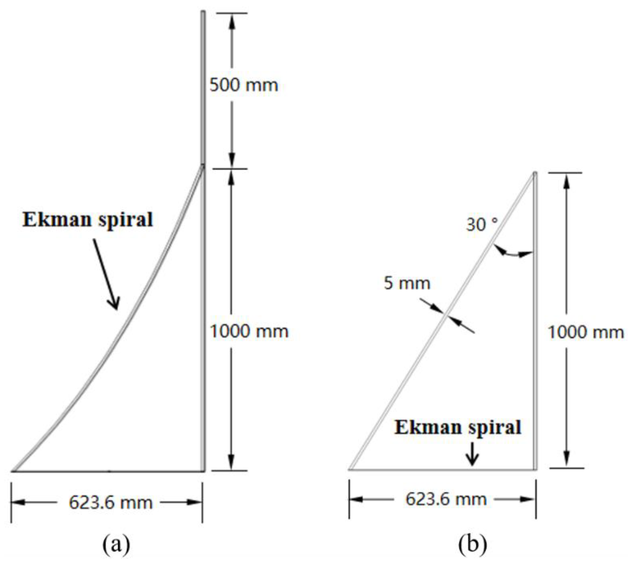
| model | Ekman spiral |
| 30° | |
| 0° | |
| 0° | |
| 1.5 m | |
| 750 mm | |
| 700 mm | |
| 3800 mm |
Disclaimer/Publisher’s Note: The statements, opinions and data contained in all publications are solely those of the individual author(s) and contributor(s) and not of MDPI and/or the editor(s). MDPI and/or the editor(s) disclaim responsibility for any injury to people or property resulting from any ideas, methods, instructions or products referred to in the content. |
© 2024 by the authors. Licensee MDPI, Basel, Switzerland. This article is an open access article distributed under the terms and conditions of the Creative Commons Attribution (CC BY) license (https://creativecommons.org/licenses/by/4.0/).
Share and Cite
Yi, Z.; Wang, L.; Li, X.; Zhang, Z.; Zhou, X.; Yan, B. Computational Fluid Dynamics-Aided Simulation of Twisted Wind Flows in Boundary Layer Wind Tunnel. Appl. Sci. 2024, 14, 988. https://doi.org/10.3390/app14030988
Yi Z, Wang L, Li X, Zhang Z, Zhou X, Yan B. Computational Fluid Dynamics-Aided Simulation of Twisted Wind Flows in Boundary Layer Wind Tunnel. Applied Sciences. 2024; 14(3):988. https://doi.org/10.3390/app14030988
Chicago/Turabian StyleYi, Zijing, Lingjun Wang, Xiao Li, Zhigang Zhang, Xu Zhou, and Bowen Yan. 2024. "Computational Fluid Dynamics-Aided Simulation of Twisted Wind Flows in Boundary Layer Wind Tunnel" Applied Sciences 14, no. 3: 988. https://doi.org/10.3390/app14030988