Abstract
The controlled source audio-frequency magnetotelluric method (CSAMT) stands out for its economic efficiency and widespread application in geophysical monitoring. However, the separate inversion of time-lapse monitoring data encounters challenges in comparing and identifying abnormal changes due to variations in data fitting. Furthermore, the utilization of a method akin to Cagniard apparent resistivity for inversion necessitates the simultaneous observation of at least two components of the electromagnetic field, making it unsuitable for extensive three-dimensional observations. This paper proposes a 3D time-lapse electric field inversion algorithm for CSAMT, addressing the complexities in geophysical monitoring. The algorithm introduces two regularization factors and defines an objective function with both temporal and spatial constraints. Synthetic testing reveals the stability of the 3D time-lapse electric field inversion algorithm, demonstrating its effectiveness in delineating underground variations. This solution resolves the challenges posed by the independent inversion of time-lapse monitoring data.
1. Introduction
Electromagnetic exploration and monitoring technology are extensively applied in various domains such as coal [1], water [2], oil [3], gas, geothermal [4], engineering [5], resource exploitation [6], scientific research [7], and environmental studies [8]. It offers technical advantages such as cost-effectiveness, efficiency, and non-invasiveness towards the monitoring target. Despite the widespread use of electromagnetic monitoring technology, challenges persist in the processing of time-lapse monitoring data. Analyzing abnormal positions in monitoring results becomes intricate due to variations in data observation conditions, noise levels, and the inversion fitting degree of the analytical method applied to detect abnormal changes in monitoring targets. Particularly during the data preprocessing stage, subjective human factors introduce variability, rendering the inversion results more challenging to compare.
Electromagnetic monitoring typically forecasts the changes in underground structures by comparing inversion results and analyzing resistivity alterations. Hu et al. [9] predicted the Sebei 2 gas reservoir by scrutinizing the resistivity residual profile using two-dimensional inversion. Xie et al. [10] employed a time-lapse long-offset transient electromagnetic sounding method to monitor oilfield waterflooding production. They identified and predicted the underground oil production range through the resistivity profile obtained via subtractive inversion. However, variations in observation equipment, changes in observation conditions, and data preprocessing adversely impact data quality. Concurrently, different noise levels in monitoring data, diverse fitting degrees of data, and the choice of a prior model significantly influence the reliability of inversion results. Consequently, the separation of inversion outcomes from time-lapse monitoring data can lead to inaccurate monitoring results. This was emphasized by Kim et al. [11], who demonstrated that the isolated inversion of monitoring data can create false anomaly blocks, thereby complicating the analysis of monitoring results.
To enhance the efficacy of inversion in highlighting changes in monitoring targets and address the challenges arising from the separate inversion of monitoring data, numerous scholars have conducted research. Daily et al. [12] employed the inversion of the ratio between the initial data set and the subsequent data set to emphasize changes in the underground electrical structure. Labrecque et al. [13] attempted to minimize the data difference between the initial data set and the subsequent data set and its difference from the response model. Loke et al. [14] rectified the initial model parameters of the inversion data in each monitoring stage to mitigate false anomaly blocks generated by inversion. Kim et al. [15] introduced a time-lapse inversion algorithm for the simultaneous inversion of multiple time observation data, capable of handling data with distinct observation times and varying noise levels. The aim is to eliminate random errors in multiple data sets and underscore changes in the underground media over time. After Kim et al. [11] proposed a 4D time-lapse inversion algorithm that put data sets and model parameters into the space–time domain, many scholars continued to study the theory of time-lapse inversion. Karaoulis et al. [16] refined the time-lapse resistivity inversion method by introducing variable time regularization factors and improving the inversion parameter optimization method. Hayley et al. [17] simultaneously inverted data sets and model parameters at multiple time points, while Loke et al. [18] utilized the smooth constrained least square method in conjunction with the L-curve parameter optimization method to enhance the speed of time-lapse inversion. Liu et al. [19] refined the time-lapse algorithm by setting inversion weights based on the quality of observation data, thereby improving inversion reliability. Hu et al. [20] applied the time-lapse inversion algorithm to the CSAMT. Through the study of the synthetic data test, it was found that time-lapse inversion cannot only eliminate false anomalies but also obtain reliable inversion results in high noise or when there is a large amount of missing observation data.
The controlled source audio-frequency magnetotelluric method (CSAMT) circumvents reliance on random weak natural field source signals, mitigates issues related to the dead band of natural field sources, and remains impervious to high-resistance shielding. This method offers advantages such as a high signal-to-noise ratio and economical observation costs. Due to the utilization of artificial sources in field construction, electromagnetic noise environments are present; nevertheless, reliable signals can still be measured. This characteristic makes it the preferred technology for electromagnetic monitoring applications. CSAMT typically defines apparent resistivity similarly to MT Cagniard apparent resistivity but is unsuitable for large-area three-dimensional observation due to the need to observe the magnetic field. The method involves the simultaneous observation of two mutually orthogonal electric and magnetic fields while sharing magnetic channels among multiple electric channels during the production process. Any loss or noise contamination in the magnetic data can impact the calculation of Cagniard apparent resistivity at multiple sites [21]. Furthermore, a deviation in the horizontal direction of the magnetic probe arrangement can introduce measurement errors in Cagniard apparent resistivity [22].
By altering the inversion strategy of the controlled source audio-frequency magnetotelluric method to exclusively utilize the electric field component for inversion, the need for magnetic field measurements is avoided. This not only avoids the issues caused by the Cagniard effect but also leads to a significant reduction in the number of sites, equipment costs, and field work expenses. Consequently, large-scale three-dimensional observations using the CSAMT become more feasible.
To address the challenge of comparing separate inversions in large-area three-dimensional measurements, a 3D time-lapse electric field inversion algorithm for CSAMT is proposed. This algorithm leverages the electric field component for inversion, reducing instrument layout requirements and rendering fieldwork more suitable for large-area three-dimensional measurements. The algorithm discontinues the calculation of Cagniard apparent resistivity, thereby avoiding potential errors in the magnetic field measurement process. The designed objective function not only incorporates model terms to impose constraints on the inversion in model space but also introduces time-lapse terms to establish connections among the inversion data at different time steps, thereby enforcing temporal constraints. A function with temporal and spatial constraints is defined, and through formula derivation and synthetic testing, the feasibility of the 3D time-lapse electric field inversion algorithm is discussed. We designed two constantly changing high and low resistivity anomalous bodies in the theoretical model. In the dynamic model, three time steps are selected to calculate the forward responses and perform synthetic data testing. Various levels of noise are introduced to the forward response for time-lapse inversion, testing the reliability of the algorithm. The synthetic test results indicate that the 3D time-lapse electric field inversion algorithm for CSAMT performs well, effectively addressing the challenge of comparing data with different noise levels. The observation method aligned with the algorithm proves suitable for large-scale three-dimensional measurements. The algorithm, which incorporates dual constraints in both temporal and spatial dimensions, demonstrates stability and feasibility in the field of monitoring.
2. Methodology
2.1. Electromagnetic Field Governing Equation
The three-dimensional forward modeling employs the staggered sampling finite difference method. Under the international system of units, the harmonic factor is expressed as . Combining this with the constitutive equation, Maxwell’s equations are derived, leading to the Helmholtz equation corresponding to the electric field (Equation (1)):
In the above formula, is the Hamiltonian operator, is the electric field strength, and , , , and represent imaginary unit, angular frequency, permeability, and conductivity, respectively. For the electric dipole source, the ground source is denoted as , where is the amplitude of transmission current, is the length of ground source, and is the unit impulse function. Singular points are formed at the field source because of the properties of the impulse function. The resistivity model is decomposed into the background model and anomaly model . The total field is obtained by the strategy of obtaining the primary field (background field) , and the secondary field separately addresses the singularity problem at these points [23]. Finally, the secondary field control equation of the frequency-domain controlled source electromagnetic method is derived (Equation (2)):
2.2. Electric Field Responses
In background model , the Fast Hankel transform is applied to calculate the primary field (background field) , as expressed in Equation (3):
where is the dipole moment, is the conductivity of half space, is the wave number, is the angular frequency, is the distance from the site to the center point of the transmitting source (i.e., the transmitter and receiver distance), and indicates the included angle between the sites and the center of the transmitting source. is the factor related to the resistivity and thickness of the layers.
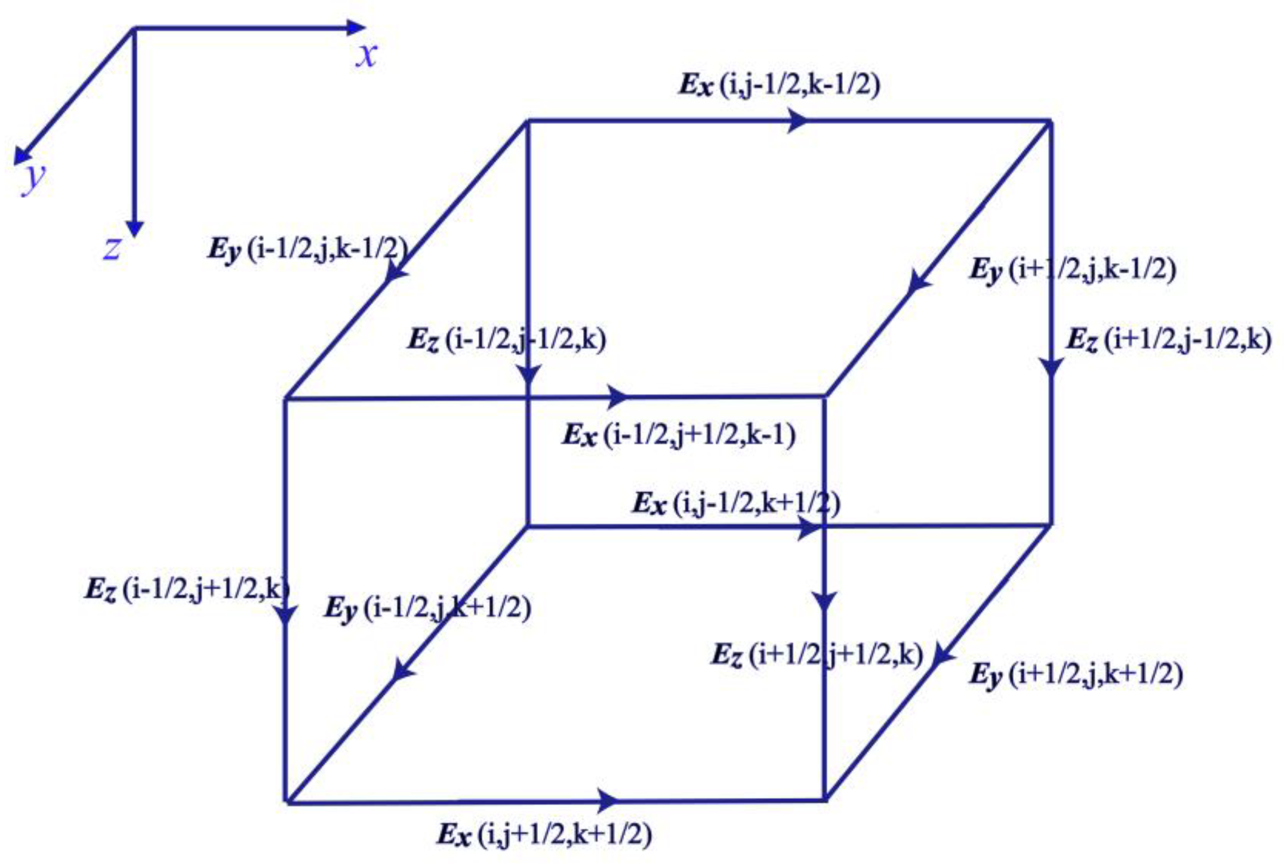
For the secondary field (induced field) in the anomaly model , the staggered grid finite difference method using the Yee grid [24] is applied. The secondary field is defined at the midpoint of the grid element edge. The staggered grid finite difference method is depicted in Figure 1.

Figure 1.
Schematic diagram of the rectangular grid of electrode cells.
The control Equation (2) is discretized in the X, Y, and Z directions. The electric field on each edge of the cells can be represented by the 12 electric field components around it. According to the rectangular grid, , equations are formed. The linear algebraic Equation (4) is obtained by finite difference discretization of rectangular grids:
In Equation (4), is a large symmetric sparse coefficient matrix, is the vector related to the boundary conditions and the primary field, and is the value of the secondary field to be solved. This study adopts the first boundary condition, also known as Dirichlet boundary condition. By employing the quasi-minimal residual method (QMR) to solve the system of Equation (4), the electric field components at each node are obtained.
2.3. Objective Function
The objective of inversion in electromagnetic exploration is to deduce the corresponding geoelectric model based on the functional relationship between observation data and geophysical model parameters. During the monitoring process of the controlled source electromagnetic (CSEM) method, dynamic changes in the underground electrical structure result in alterations to the electric field responses measured on the ground. The mapping relationship between the electric field values observed at different times and the resistivity model at the corresponding time is established for inversion. The 3D time-lapse electric field inversion algorithm for the controlled source audio-frequency magnetotelluric method (CSAMT) is defined as follows (Equation (5)):
where is the data fitting residual term, is the model smoothness constraint term, is the time-lapse constraint item of the model, and and are regularization factors.
2.3.1. Data Fitting Residual Term and Model Term
The data fitting residual term is defined by the following equation (Equation (6)):
The model term is defined by the following Equation (7):
In Equations (6) and (7), is the observed electric field response dataset, with dimensions of . refers to the number of data at one time step, refers to the number of time steps, and is the electric field response data measured at time step. is forward response; is the data weighting matrix: . is the resistivity parameter of the model corresponding to each observation time step. is the reference model resistivity parameter. is an iterative, and the dimensions of and are . represents the number of rectangular grids, and is the linear smooth matrix of the model.
2.3.2. Time Lapse Term
Time-lapse inversion constrains the changes in models over time by introducing a time-lapse term to the objective function. The time-lapse term is defined as follows (Equation (8)):
where is the model parameter at time step , is the coefficient matrix, and the expression is given in Equation (9), where is the total number of measured time steps. The time-lapse term establishes connections between spatial models at different time steps. Each iteration simultaneously inverts the observation data at time steps and obtains the underground electrical structure model at time steps. The mutual constraint of the observation data at each time step facilitates the realization of the time constraint effect.
2.3.3. Regularization Factor
The Tikhonov regularization method [25] has gained widespread acceptance and application for addressing ill-posed inverse problems. Regularized inversion mitigates the multiplicity of solutions by incorporating model constraints into the objective function. The regularization factor serves as the compromise coefficient between the data fitting function and the model stability function. A higher value of the regularization factor emphasizes model constraint, often resulting in underfitting of the data [26]. Conversely, a lower value of the regularization factor indicates a bias towards data fitting, potentially leading to false structure due to the influence of data noise, commonly known as overfitting. Therefore, the choice of the regularization factor significantly impacts the inversion outcome, playing a pivotal role in the inversion effect [27].
The symbol represents the regularization factor of the time-lapse term and mathematically signifies the weight of the time-lapse term’s influence on the inversion result. controls the similarity between models at each time step, representing temporal constraints. In this algorithm, is set to a fixed scalar value, indicating that the differences between models do not change in the time dimension. A larger value implies a closer iterative trend model, suggesting minimal differences between models at each time step. Conversely, a smaller value reduces the weight of the time-lapse term’s influence on inversion results, allowing greater differences in model changes at each time during the iteration process. When calculating measured data, the value of can be determined based on the variance of the electric field response section at each time step.
The effect of aligns with that of the Tikhonov regularization factor. To achieve both data fitting and dual constraints of temporal and spatial considerations, λ is gradually decreased when the number of iterations increases and the root-mean-square (RMS) of the data fitting difference no longer decreases. This reduction in λ is expressed by Formula (10):
2.3.4. Data Fitting Difference Formula
The parameter reflecting the quality of inversion results, the root-mean-square (RMS) misfit, is defined as follows (Equation (11)), where denotes the total number of sites. The parameter α serves as a given data deviation used to assess the reliability of the measured data. In ideal circumstances, the disparity between the forward response and the measured data should be zero. A smaller value of α indicates higher data reliability, while a larger initial RMS necessitates an increase in the number of iterations for the inversion to enhance the fitting degree.
2.4. Time Lapse Inversion
2.4.1. Gradient of the Objective Function
The inversion algorithm in this study adopts the nonlinear conjugate gradient (NLCG) method, with the gradient derived based on the research findings of Lin et al. [28]. To avoid computational errors caused by the increasing number of inversion time steps leading to the accumulation of gradients, the gradients were normalized based on the number of time steps. The gradient representation of the objective function for the 3D time-lapse electric field inversion algorithm for CSAMT is given by the following Equation (12):
To address the challenges of computing the Jacobian matrix for obtaining the gradient of the objective function, the classical “pseudo-forward” method is employed to overcome the difficulties associated with directly solving for the Jacobian matrix.
2.4.2. The Process of 3D Time-Lapse Electric Field Inversion
The general process of the 3D time-lapse electric field inversion algorithm for CSAMT can be roughly divided into the following four steps:
- 1.
- Import data: Inversion parameters such as regularization factors λ and β, minimum fitting error ε, observed data D, model parameters M, and prior model parameters ;
- 2.
- Forward modeling: Calculate the electric field response for each time-lapse model;
- 3.
- Iteration assessment: Evaluate the objective function and determine the termination condition for inversion based on the root-mean-square being less than .
- 4.
- Model update: Utilize the gradient of the objective function in Equation (12). By choosing the negative gradient direction as the descent direction for the objective function to calculate the search direction p, update the step length α, and then update the model parameters using the formula m = m + αp. The detailed calculation process refers to Figure 2.
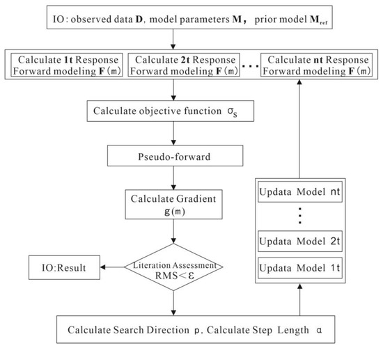 Figure 2. Flow of time-lapse electric field inversion algorithm.
In this algorithm, the minimum fitting error is set to 1.05. When the RMS reaches the minimum fitting error of 1.05, the program determines that the inversion result is closest to the true underground situation and terminates the iteration.
3. Synthetic Test
Synthetic data testing was conducted on a Linux system using the IFort compiler for compilation. The device’s CPU model is AMD5950X, and it has a memory capacity of 128 GB.
Various levels of noise were introduced to the theoretical responses, and a 3D time-lapse electric field inversion algorithm for CSAMT was executed with varying noise levels and inversion parameters. The stability and reliability of the testing algorithm, along with the impact of time-lapse terms, were assessed. During the monitoring process, the noise level of the measured data is subject to variation due to changes in instrument status, measurement environment, and human electromagnetic noise. Hence, it is essential to conduct inversion tests on algorithms using various noise data or noise pollution data. The levels of added noise and the inversion parameters are detailed in Table 1.

Table 1.
Testing data noise levels and inversion parameters.
3.1. Layout of Survey and Time-Lapse Model
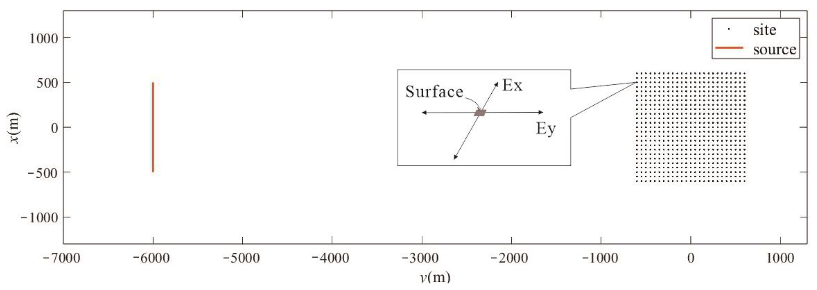
The simulated survey layout is depicted in Figure 3. The center of the transmitting source is situated at 6000 m in the x-direction, with a length of 1000 m and a power supply current of 10 A, indicated by the red line in the figure. There are 25 survey lines, each spanning 1200 m and comprising 25 sites per line, spaced 50 m apart, totaling 625 sites, as denoted by the black dots in the figure. The simulated observations span 18 frequencies ranging from 8192 to 0.1 Hz (8192, 4096, 2048, 1280, 640, 320, 160, 80, 64, 32, 16, 8, 4, 2, 1, 0.5, 0.25, 0.1).
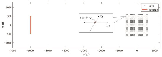
Figure 3.
Schematic diagram of the layout.
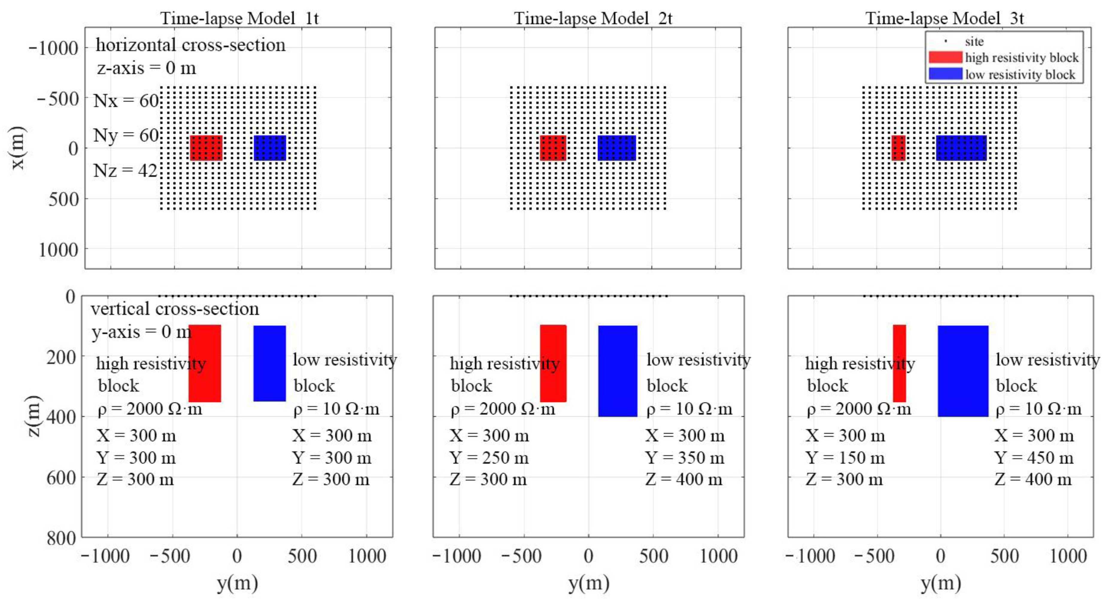
In the dynamic model of the time-lapse model containing high and low resistivity anomaly blocks, 1t, 2t, and 3t time steps are selected for CSAMT forward and time-lapse electric field inverse testing. The relationship between the scale of the resistivity anomalies and the site positions at three time steps is illustrated in Figure 4.

Figure 4.
Relationship between the time-lapse model’s resistivity anomaly blocks and the positions of the sites.
In Model O, within a background stratum of 100 Ω·m, a model is constructed featuring a high-resistivity block of 2000 Ω·m with a continuously decreasing scale and a low-resistivity block of 10 Ω·m with a continuously increasing scale, as illustrated in Figure 4. Nx, Ny, and Nz represent the number of grids employed for the purpose of discretization. The forward calculation of three time-step models employs the identical grid discretization. The background medium is omitted in the figure, with only the varying subsurface media displayed.
3.2. Time-Lapse Data Synthesis
Comparing independent inversion results may be challenging due to variations in noise levels and fitting degrees. Particularly, significant contamination of the data with noise at specific instances can result in inaccurate monitoring outcomes. We introduced noise of comparable magnitude to simulate smooth monitoring, incorporate elevated noise levels to replicate noise pollution data, and simulate monitoring failures. We performed numerous tests using synthetic data to assess the algorithm’s stability, its capability to address the challenge of comparing monitoring results, the reliability of pollution data, and the influence of inversion parameters on the outcomes.
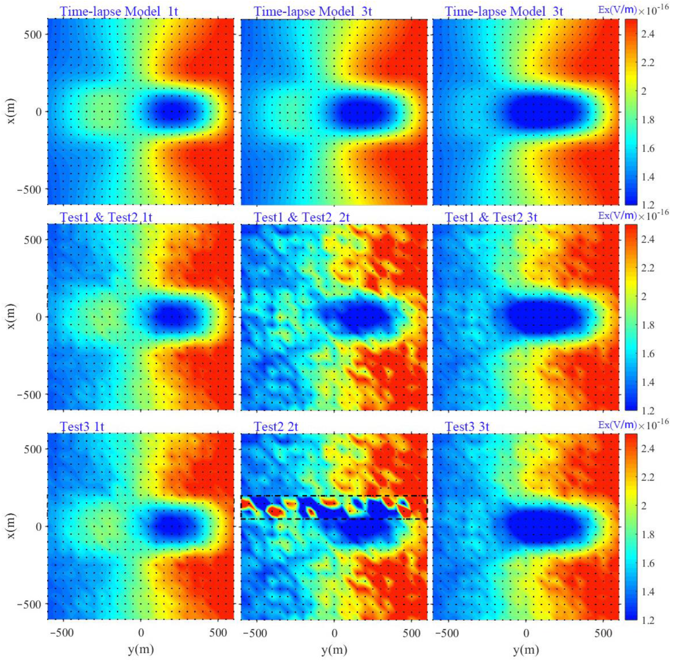
Figure 5 presents the synthetic data used for the time-lapse model and algorithm testing, with the black dots indicating the positions of the observation sites. Time-lapse Model 1t, Time-lapse Model 2t, and Time-lapse Model 3t represent the slices of the forward responses (Ex = 16 Hz) at three different time steps for the time-lapse model. Gaussian noise at levels of 2%, 8%, and 5% was added to the forward responses of the three time steps for the time-lapse model at 18 frequencies. Two different time-lapse inversions, Test 1 and Test 2, were conducted with different inversion parameters to discuss the time constraint effect of the time-lapse term. The noise level of Time-lapse Model 2t was increased to 50% for Test 3, addressing the anti-noise effect of the time-lapse inversion.
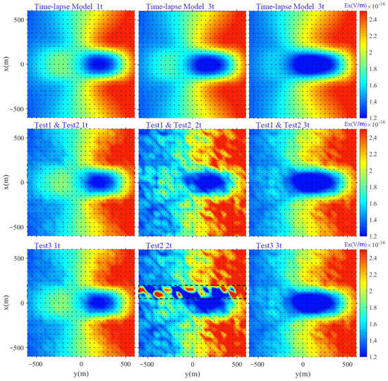
Figure 5.
Changes in the forward response of the time-lapse model electric field and noise data (Ex = 16 Hz).
3.3. Inversion Results for Time-Lapse
3.3.1. Inversion Parameters
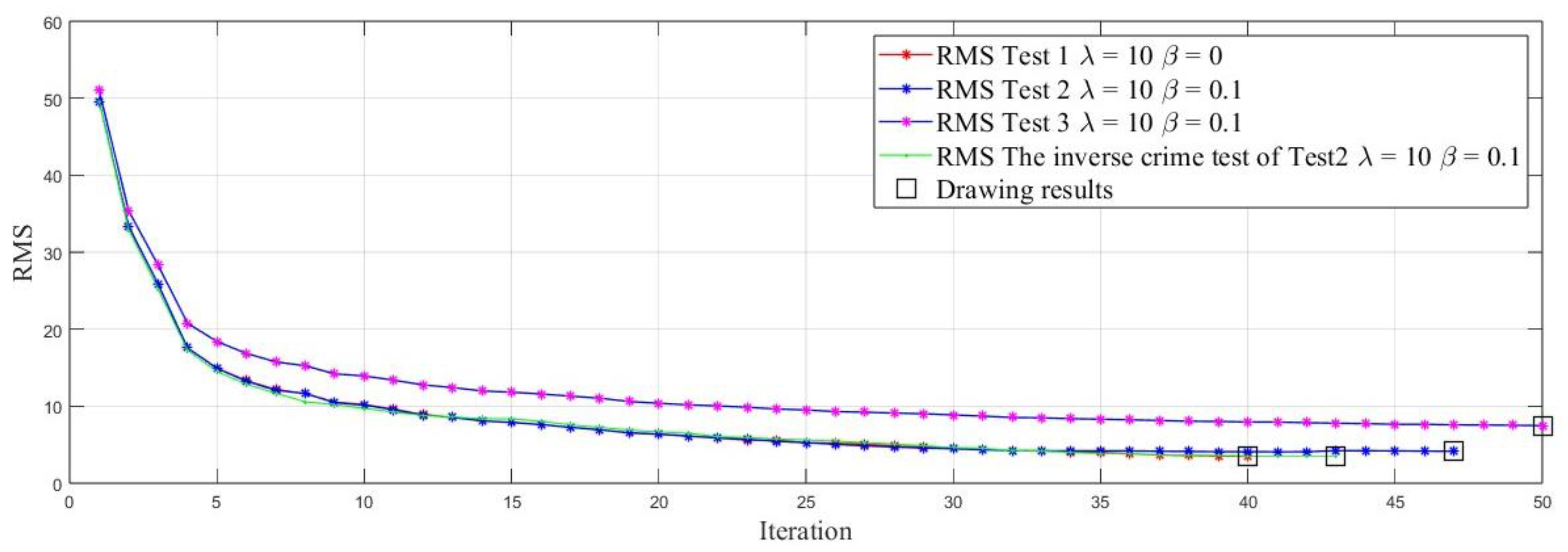
Theoretically, when RMS = 0, the resistivity model derived from inversion aligns with the underground resistivity distribution. However, it is not possible to achieve an inversion result with RMS = 0 due to the presence of noise. Figure 6 illustrates a smooth decrease in RMS with an increasing number of iterations, along with a smooth descent curve. This indicates the stable convergence of the inversion process and reflects the stability of the algorithm.
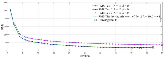
Figure 6.
RMS reduction curve with iteration count.
Analyzing the RMS reduction curves of Test 1 and Test 2 in Figure 6 reveals that the incorporation of the time-lapse regularization factor β decelerates the rate of RMS reduction in data fitting. This phenomenon can be attributed to the diminished influence of the data term in the inversion process, a consequence of integrating the time-lapse term. In the synthetic data test, the deviation value α remains constant. However, in Test 3, certain measurement points are impacted by high noise, leading to a higher initial RMS value compared to Test 1, as depicted in Equation (11). Test 3 underscores the challenge of fitting high-noise data, resulting in a more gradual reduction in RMS.
Based on the selected plotting results in Figure 6, profiles at z = 200 m and x = 0 are separately depicted in Figure 7. In Figure 7, the red box corresponds to the range of high-resistivity anomaly blocks at each time step, while the blue box corresponds to the range of low-resistivity anomaly blocks. The results indicate that the 3D time-lapse electric field inversion algorithm for CSAMT has, to varying degrees, recovered the positions and resistivity values of the designated high and low resistivity anomaly blocks.
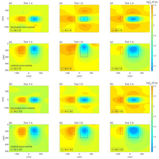
Figure 7.
Synthetic data testing results for the time-lapse electric field inversion. (a) The red and blue boxes represent the theoretical locations; Nx = 60, Ny = 60, Nz = 42. (b) The red and blue boxes represent the theoretical locations; Nx = 60, Ny = 60, Nz = 42.
Figure 7a displays the inversion results of Test 1 with β = 0, where the time-lapse term does not impact the inversion results. Figure 7b illustrates the inversion results of Test 2 with a time lapse factor of 0.1. When comparing the horizontal slice results in the two figures, it is observed that the high resistivity volume range within the red box is closer to the theoretical position, and the false anomaly range around the blue box is significantly reduced. β is a regularization factor that theoretically spans from 0 to ∞. However, if the value is excessively large, it prevents the inversion from converging, whereas if it is too small, it fails to provide a constraining effect. Upon examining Figure 6, it is evident from the RMS descent curves of Test 1 and Test 2 that the inclusion of a time-lapse term hampers the convergence rate of the inversion process. Despite Test 1 having a lower RMS value compared to Test 2, the results of Test 2 align more closely with the theoretical model, suggesting that the time-lapse term facilitates the inversion process.
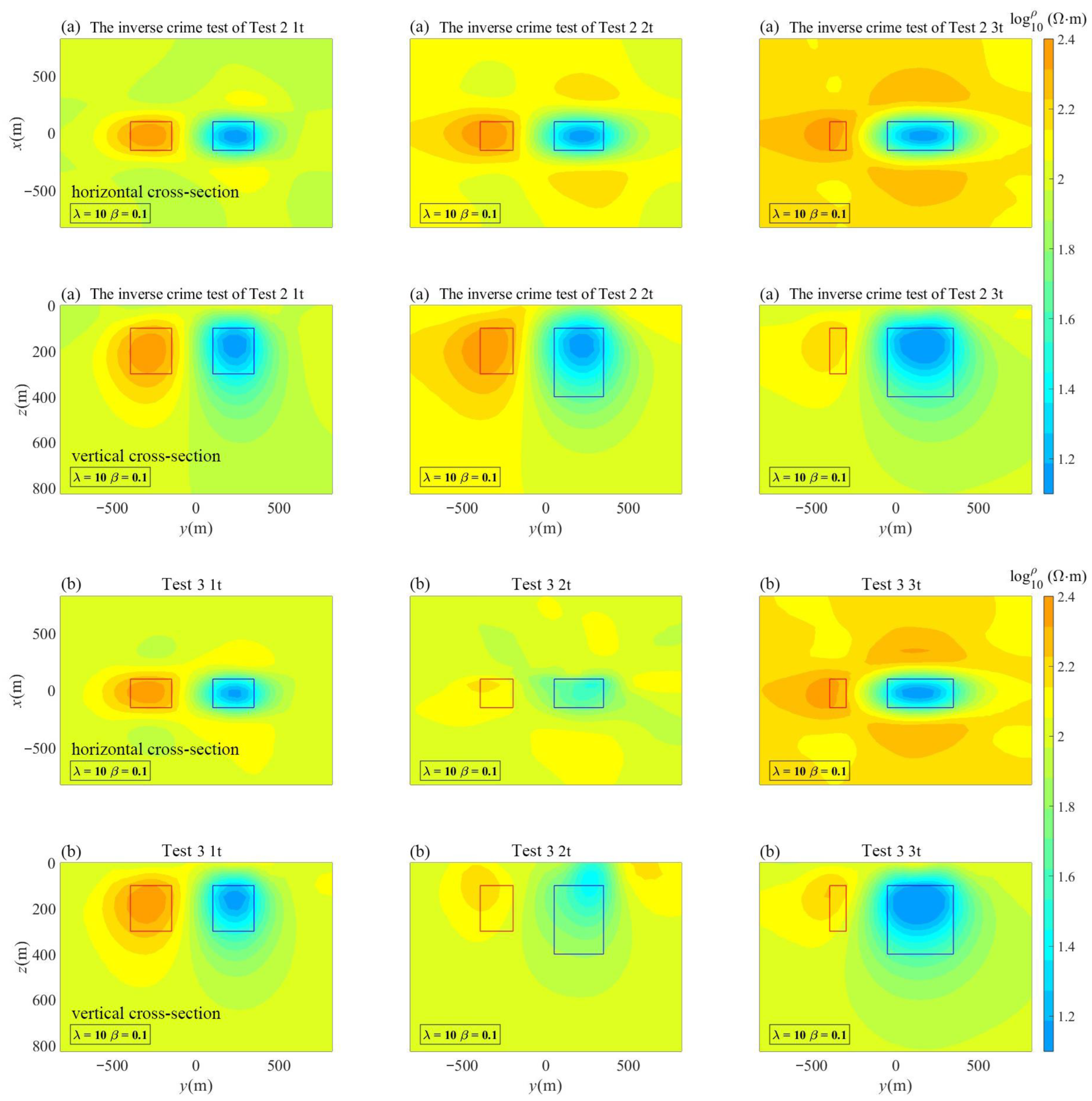
We evaluated the algorithm’s effectiveness in mitigating inverse crime [29] by varying the grid size and number and performing the time-lapse electric field inversion in Test 2. The inversion results are depicted in Figure 8a. The algorithm demonstrates stability and does not exhibit any prominent issues of inverse crime. Figure 6 depicts the RMS decline curve of the inversion crime test, represented by the green curve.
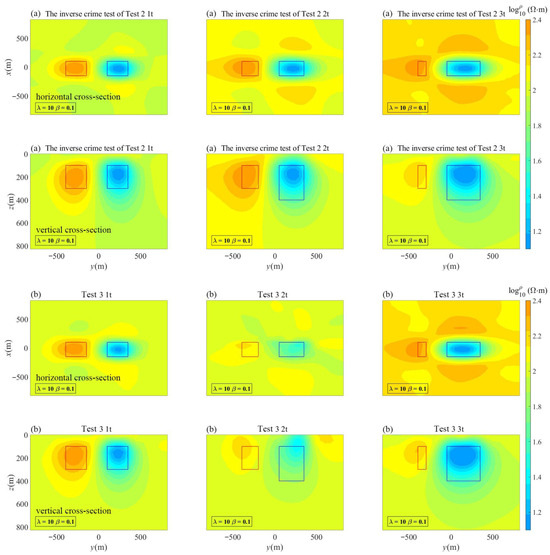
Figure 8.
Synthetic data testing results for the time-lapse electric field inversion (The red and blue boxes represent the theoretical locations; (a) Nx = 60, Ny = 60, Nz = 42; (b) Nx = 62, Ny = 62, Nz = 44).
In Figure 8b, the data yielded in Test 3 were highly noisy and polluted, and the time-lapse inversion accurately recovered the locations of high and low resistivity anomaly bodies. Moreover, in Test 3, the time-lapse data at three different noise levels, 1t, 2t, and 3t, were iteratively inverted simultaneously, mitigating the challenge of comparing independently inverted data at each time step due to varying fitting degrees.
3.3.2. Results and Discussion
In the objective function, λ controls the smoothness of the model in spatial terms, with a larger value resulting in a smoother inverted model. On the other hand, β governs the degree of temporal variation in the model. A comparative analysis of the inversion results of Test 1 and Test 2 reveals that the time-lapse term enhances the inversion accuracy. A larger β value suppresses changes in the model at adjacent time steps, yielding more similar inversion results at each time step. Conversely, a smaller β value imposes fewer constraints on the model at each time step, allowing for more liberal changes in the model at adjacent time steps. The inclusion of the time-lapse term in the results of Test 2 not only improves the accuracy of recovering the low-resistivity anomaly block but also reduces false anomalies around the blue box. Temporal constraints holds great significance for monitoring purposes as they not only enhance the ability to identify anomalies but also enable a more efficient comparative analysis of the monitoring results.
The time-lapse calculation represents the disparity between model parameters, while the weight in inversion aims to minimize the discrepancy between the models. Thus, even when the data are heavily contaminated with noise, accurate results can still be obtained through the process of inversion.
4. Conclusions
The conclusions drawn from the synthetic data testing of the 3D time-lapse electric field inversion algorithm for CSAMT are as follows:
The algorithm, incorporating dual constraints in both temporal and spatial dimensions, demonstrates stability and feasibility, exhibiting robust performance in inverting monitoring data across various noise levels. The algorithm demonstrated its reliability by adjusting the size and number of discrete grid cells without significant inversion crime issues. By implementing time-lapse inversion on the observational data at each time step, the algorithm effectively addresses the challenge posed by the separate inversion of the monitoring data, enhancing the comparability of the results. Independent inversion, particularly when handling noise pollution data, is susceptible to generating inaccurate monitoring outcomes. Conversely, time-lapse inversion can be executed seamlessly, showcasing commendable performance under the combined influences of temporal and spatial constraints.
Directly inverting a single electric field component, without the need for calculating the Cagniard apparent resistivity, yields reliable inversion results. This implies that during field operations, the monitoring objectives of the controlled source audio-frequency magnetotelluric method can be attained by observing only a single component of the electric field. The technology of CSAMT monitoring combined with this algorithm is well-suited for large-scale three-dimensional measurements in a diverse environment.
Author Contributions
Methodology and writing—original draft preparation, Q.S.; writing—review and editing, project administration, H.T.; software, W.W.; validation, Q.H. All authors have read and agreed to the published version of the manuscript.
Funding
This study was supported by the National Natural Science Foundation (Grant Nos. 41830429 and 42004123) and the Hubei Zigui–Changyang Shale Gas Strategic Area Survey Project (Grant No. DD20179623).
Institutional Review Board Statement
Not applicable.
Informed Consent Statement
Not applicable.
Data Availability Statement
The raw data supporting the conclusions of this article will be made available by the author Qilong Sun on request.
Conflicts of Interest
No conflict of interest exists in the submission of this manuscript.
References
- Ning, Z.; Mingwei, H.; Yahang, S.; Deqiang, T.; Ce, Q. Forward modeling of 3D DC resistivity based onhigh-order adaptive finite element and its applicationin Qinshui Basin. Oil Geophys. Prospect. 2021, 56, 209–216. [Google Scholar]
- Jin, Y.; Oingcheng, L.; Yexun, C.; Nanping, W.; Shengli, H. The Application of Environmental Geophysics in Inspecting Groundwater Contamination. Res. Environ. Sci. 1998, 11, 43–46. [Google Scholar] [CrossRef]
- Su, Z.; Yang, Z.; Li, H.; Hu, W.; Qin, Z.; Yan, L. Application of Electric Potential Method (EPM) in Dynamic Monitoring of Reservoirs. J. Oil Gas Technol. 2006, 28, 56. [Google Scholar]
- Legaz, A.; Vandemeulebrouck, J.; Revil, A.; Kemna, A.; Hurst, A.W.; Reeves, R.; Papasin, R. A case study of resistivity and self-potential signatures of hydrothermal instabilities, Inferno Crater Lake, Waimangu, New Zealand. Geophys. Res. Lett. 2009, 36, L12306. [Google Scholar] [CrossRef]
- Bhuyian, A.H.; Landrø, M.; Johansen, S.E. 3D CSEM modeling and time-lapse sensitivity analysisfor subsurface CO2 storage. Geophysics 2012, 77, E343–E355. [Google Scholar] [CrossRef]
- Yan, L.J.; Chen, X.X.; Tang, H.; Xie, X.B.; Zhou, L.; Hu, W.B.; Wang, Z.X. Continuous TDEM for monitoring shale hydraulic fracturing. Appl. Geophys. 2018, 5, 26–34. [Google Scholar] [CrossRef]
- Grayver, A.V.; Streich, R.; Ritter, O. 3D inversion and resolution analysis of land-based CSEM data from the Ketzin CO2 storage formation. Geophysics 2014, 79, 820–830. [Google Scholar] [CrossRef]
- Karaoulis, M.; Revil, A.; Tsourlos, P.; Werkema, D.D.; Minsley, B.J. A software for time-lapse 2D/3D DC-resistivity and induced polarization tomography. Comput. Geosci. 2013, 54, 164–170. [Google Scholar] [CrossRef]
- Zuzhi, H.; Dechun, L.; Yunxiang, L.; Weibin, S.; Caifu, W.; Yongtao, W. Reservoir monitoring feasibility study with timelapse magnetotelluric survey in Sebei Gas Field. OGP 2014, 49, 997–1005. [Google Scholar]
- Xingbing, X.; Lei, Z.; Liangjun, Y.; Wenbao, H. Remaining oil detection with time-lapse long offset & window transient electromagnetic sounding. OGP 2016, 51, 605–612. [Google Scholar]
- Kim, J.H.; Yi, M.J.; Park, S.G.; Kim, J.G. 4-D inversion of DC resistivity monitoring data acquired over a dynamically changing earth model. J. Appl. Geophys. 2009, 68, 522–532. [Google Scholar] [CrossRef]
- Daily, W.; Ramirez, A.; LaBrecque, D.; Nitao, J. Electrical resistivity tomography of vadose water movement. Water Resour. Res. 1992, 28, 1429–1442. [Google Scholar] [CrossRef]
- LaBrecque, D.J.; Yang, X. Difference inversion of ERT data: A fastinversion method for 3-D in situ monitoring. J. Environ. Eng. Geophys. 2001, 6, 83–89. [Google Scholar] [CrossRef]
- Loke, M.H. Time lapse resistivity imaging inversion. In Proceedings of the 5th Meeting of the Environmental end Engineering European (Em1), Budapest, Hungary, 5–9 September 1999. [Google Scholar]
- Kim, J.-H. Four dimensional inversion of dc resistivity monitoring data. In Proceedings of the Near Surface 2005—11th European Meeting of Environmental and Engineering Geophysics, Palermo, Italy, 4–7 September 2005; European Association of Geoscientists and Engineers: Utrecht, The Netherlands, 2005; p. A006. [Google Scholar]
- Karaoulis, M.C.; Kim, J.H.; Tsourlos, P.I. 4D active time constrained resistivity inversion. J. Appl. Geophys. 2011, 73, 25–34. [Google Scholar] [CrossRef]
- Hayley, K.; Pidlisecky, A.; Bentley, L.R. Simultaneous time-lapse electrical resistivity inversion. J. Appl. Geophys. 2011, 75, 401–411. [Google Scholar] [CrossRef]
- Loke, M.H.; Dahlin, T.; Rucker, D.F. Smoothness-constrained time-lapse inversion of data from 3D resistivity surveys. Near Surf. Geophys. 2014, 12, 5–24. [Google Scholar] [CrossRef]
- Bin, L.; Liu, Z.; Li, S.; Fan, K.; Nie, L.; Zhan, X. An improved Time-Lapse resistivity tomography to monitor and estimate the impact on the groundwater system induced by tunnel excavation. Tunn. Undergr. Space Technol. 2017, 66, 107–120. [Google Scholar]
- Qixuan, H.; Handong, T.; Cui, Y. 3D Inversion of Time-lapse Controlled Source Audio-frequency Magnetotellurics. Geoscience 2021, 156, 1000–8527. [Google Scholar]
- Wan, W.; Tang, X. Comparative analysis Ex, apparent resistivity and Ex/Hy, ratio apparent resistivity in CSAMT. Geophys. Ceohem. Explor. 2015, 39, 567–571. [Google Scholar] [CrossRef]
- Yang, S.H. Topographic Effect in CSAMT & Compare of Terrain Correction Methods. Master’s Thesis, China University of Geosciences, Beijing, China, 2005. [Google Scholar]
- Newman, G.A.; Alumbaugh, D.L. Frequency-domain modelling of airborne electromagnetic responses using staggered finite differences. Geophys. Prospect. 1995, 43, 1021–1042. [Google Scholar] [CrossRef]
- Yee, K. Numerical solution of initial boundary value problems involving maxwell’s equations in isotropic media. IEEE Trans. Antennas Propag. 1966, 14, 302–307. [Google Scholar]
- Tikhonov, A.N. Regularization of incorrectly posed problems. Sov. Math. Dokl. 1963, 4, 1624–1627. [Google Scholar]
- Oldenbury, D.; Li, Y. Inversion for applied geophysics: Atutorial. Near Surf. Geophys. 2005, 5, 89. [Google Scholar]
- Zhdanov, M.S. Geophysical Inverse Theory and Regularization Problems; Elsevier: Amsterdam, The Netherlands, 2002. [Google Scholar]
- Lin, C.H.; Tan, H.D.; Shu, Q.; Tong, T.; Tan, J.Y. Three-dimensional conjugate gradient inversion of CSAMT data. Chin. J. Geophys. 2012, 55, 3829–3838. [Google Scholar] [CrossRef]
- Wirgin, A. The inverse crime. arXiv 2004, arXiv:math-ph/0401050v1. [Google Scholar]


Disclaimer/Publisher’s Note: The statements, opinions and data contained in all publications are solely those of the individual author(s) and contributor(s) and not of MDPI and/or the editor(s). MDPI and/or the editor(s) disclaim responsibility for any injury to people or property resulting from any ideas, methods, instructions or products referred to in the content. |
© 2024 by the authors. Licensee MDPI, Basel, Switzerland. This article is an open access article distributed under the terms and conditions of the Creative Commons Attribution (CC BY) license (https://creativecommons.org/licenses/by/4.0/).