Article

Investigations into Higher-Frequency Hysteresis Current Controller for Supraharmonic Hybrid Active Filters

1
Department of Electrical Power System, Kaunas University of Technology, 51394 Kaunas, Lithuania
2
Department of Electrical Engineering, University of Energy and Natural Resources, P.O. Box 214 Sunyani, Ghana
*
Author to whom correspondence should be addressed.
Appl. Sci. 2024, 14(5), 1713; https://doi.org/10.3390/app14051713
Submission received: 18 January 2024 / Revised: 14 February 2024 / Accepted: 15 February 2024 / Published: 20 February 2024
(This article belongs to the Section Electrical, Electronics and Communications Engineering)

Abstract

:
Hysteresis current controllers (HCCs) are extensively used in low-frequency power inverters and active power filters. Very little is known about their strengths and weaknesses when applied at supraharmonic frequencies. The major concern regarding the use of HCCs is their variable and uncontrollable switching frequencies. This results in difficulties in filter design, high switching losses, and the possibility of resonance conditions with power system elements. In this article, investigations are conducted on the application of HCCs in a hybrid filter for a 6 kHz matrix converter (MC)-coupled supraharmonic load. The effects of the MC-coupled load and VSC switches on the HCC’s switching frequency are analyzed. A novel mathematical model for obtaining a fixed-frequency HCC is presented. The model is verified in open- and closed-loop HCC control configurations for a three-phase hybrid active power filter (HAPF). Fast Fourier transform (FFT) analysis of the supply current after the implementation of the novel HCC-HAPF showed 2.31% of the 50 Hz fundamental. The analysis is verified in a MATLAB/Simulink environment.

1. Introduction

In recent years, the use of power electronic converters as interfaces for domestic and industrial loads has increased exponentially. Wind power applications, solar photovoltaic generators, electric vehicles, and battery storage chargers are the most common applications of power electronic converters [1]. These self-commutating converters, due to their numerous switching states, have switching frequencies in the kilohertz (kHz) band range and produce switching harmonic frequencies above 2 kHz [2]. Unfortunately, very little research has been conducted, and there are few regulations on such frequency ranges. Supraharmonic frequency is a term describing harmonic frequencies between 2 and 150 kHz and was introduced by the IEEE at their PES conference in 2013 [3]. The presence of supraharmonic frequencies poses threats to power electronic converters [4].
Supraharmonic interference received less attention due to the limited use of fast switching converters in the past [5]. But with the recent high demand for electric vehicles, wireless and fast battery charging stations, variable-speed drives, and electronically controlled lamps [6], there is a need to increase research in this area. Table 1 shows the operating frequency ranges of electronic converters used for selected domestic and industrial loads.
Active power filters are preferred for harmonic compensation due to their compatibility and smaller weight and size [7,8,9,10]. Traditional passive filters may not be practical in applications where size and weight are of much concern. The IEEE Std. 519-2022 recommends an acceptable 5% THDi harmonic current distortion. Hence, the average attenuation of a passive filter should be 26 dB during maximum currents and 32 dB during minimum currents. Passive filter components based on the above are too large and bulky in applications where size and weight are of much concern. The minimum weight of a similar filter with 107 amperes of nominal choke current from the Schneider electronics ‘Altivar61’ line chokes catalogue for a three-phase source at 380 to 480 V and 50/60 Hz is 16 kg [11], which is too large for applications in aircraft, ships, electric vehicles, etc. Active harmonic filters on their own may not be an economically feasible option for higher-frequency compensation. Hybrid harmonic filters are the most viable option for supraharmonic-frequency compensation [12]. Using hybrid harmonic compensation, the parallel combination of a passive L-C filter and a shunt active power harmonic filter is proposed. With this, the passive filter is designed to attenuate 60% of the supraharmonic frequencies.
The HCC method, due to the stability and faster dynamic responses of HCCs during transient behaviors, is the most preferred pulse width modulation (PWM) control technique for active power filters. However, the variable nature of the HCC switching frequency increases switching oscillations, electromagnetic interference (EMI), and difficulty in active filter design. Most research works are on fixed-frequency HCCs for low-frequency applications [13,14,15,16]. The principle of fixed-frequency HCCs is used to define a variable hysteresis band for each leg of the VSC, thereby maintaining a nearly constant switching frequency. The behaviors of HCCs in supraharmonic frequency ranges are unknown, and not enough research has been conducted on this topic. This leaves a knowledge gap related to the feasibility of HCCs for higher-switching-frequency converters as well as the switches appropriate for its realization.
This article bridges this knowledge gap and presents a novel mathematical expression for estimating the maximum switching frequency of an HCC for hybrid active power filters (HCC-HAPF). This article presents an improved model for implementing fixed-frequency HCCs and explores its realization using metal–oxide–semiconductor field-effect transistors (MOSFETs). The dV/dt and dI/dt are analyzed, as they are the major causes of oscillations, overshoots, and EMI during higher-frequency switching.
The objectives and contributions of this study are as follows:
  • To investigate the nature and propagation of the supraharmonic frequencies produced by a 50 kW, 6 kHz MC-interfaced load.
  • To obtain a novel equation for estimating a fixed-frequency hysteresis current controller in higher-frequency applications.
  • To achieve supraharmonic frequency compensation within the recommended standards of IEEE Std. 519-2022 [17] using the HCC-HAPF.
The remainder of this paper is arranged as follows: Section 2 describes reference current generation using the P-Q technique. Section 3 reviews the HCC and derives the novel mathematical expression for the hysteresis current controller. The effects of the load and VSC switches on the switching frequency are also analyzed. The novel expression is tested with a hybrid active filter topology for a 6 kHz MC application, and Section 4 summarizes the simulation results. Section 5 discusses and compares the obtained results. Section 6 concludes the study with future research directions.

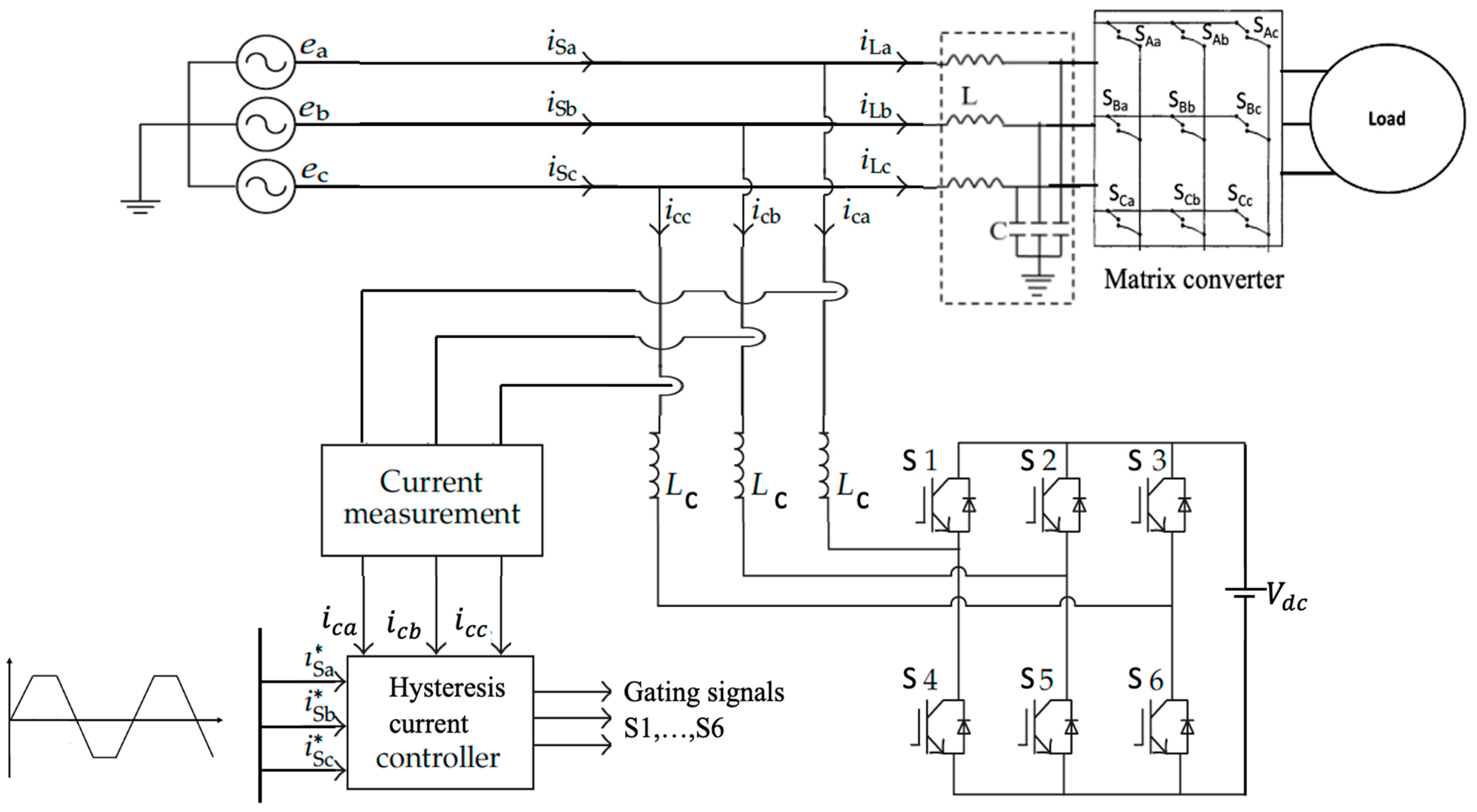
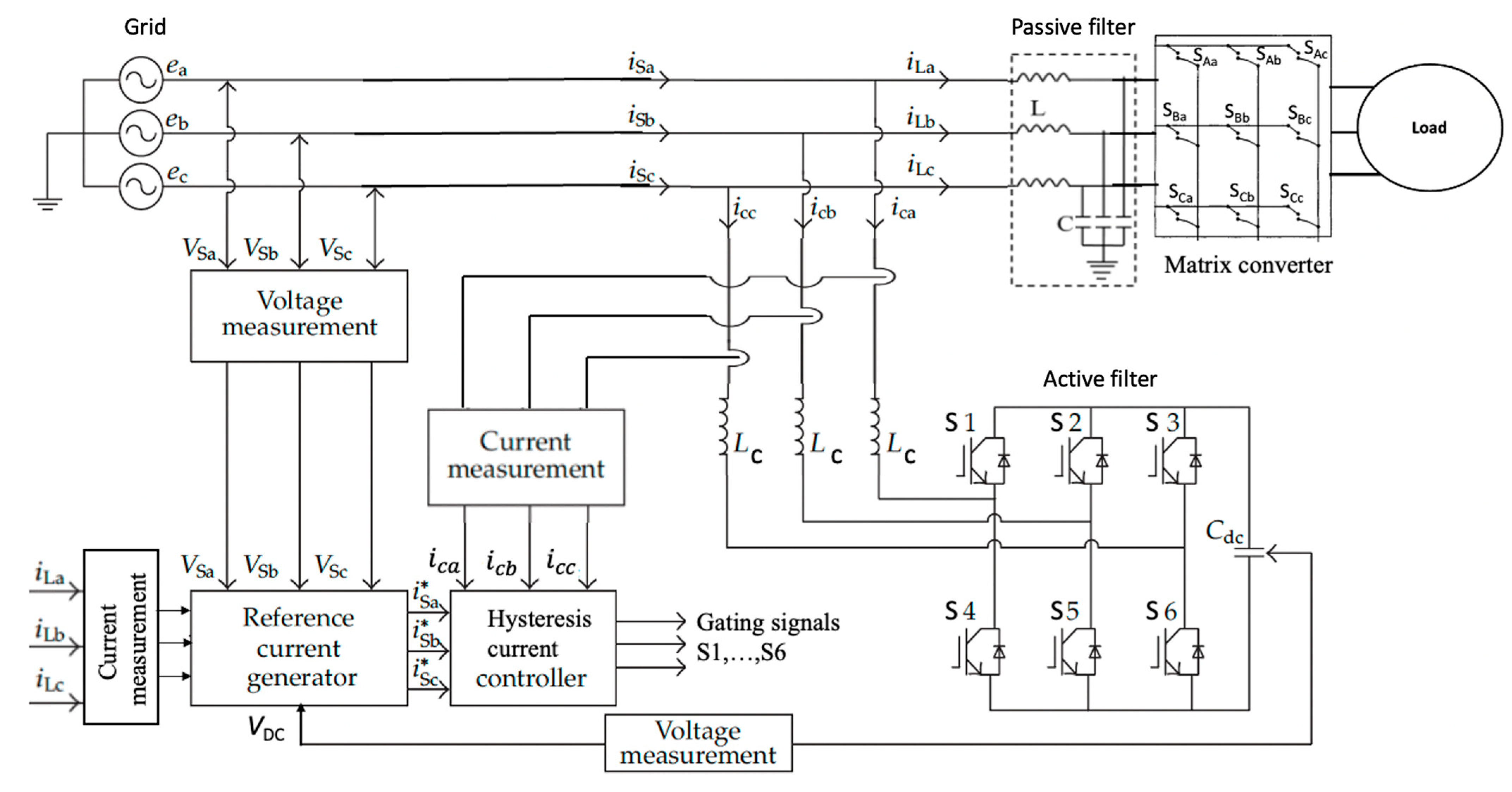
2. The MC and Supraharmonics

Several research works [1,3,6,18] have identified the sources of these supraharmonics as power electronic converters with higher switching frequencies. The authors in [1] presented supraharmonics propagation from electric vehicles with respect to small and low-voltage grids. They concluded that supraharmonic frequencies may result in the tripping of residual current devices and “frequency beating”. The authors in [3,6] seek to establish standardization and measurements for supraharmonic applications. They concluded that the emissions from supraharmonic frequencies reduce the efficiency and life expectancy of electrical equipment.
Power electronic converters are also the primary victim of supraharmonic frequencies, as their dynamic performance are crippled, as the authors in [4,5,19,20] explored. The authors in [4,5] explored the power electronic converters and supraharmonics and [17] confirmed the effect of higher harmonic frequencies as the reduction in lifespan of power system devices. The authors in [8] successfully modeled the emissions from supraharmonic devices from the parallel operation of two converters and confirmed that it can be predicted by linear models.
The advantages of the use of MCs supersedes that of the traditional back-to-back converters [21,22]. Paramount is its bi-directional operation and the absence of energy storage elements. Irrespectively, the MC’s voltage transfer ratio of 0.867 and supraharmonic input and output frequencies discourages its use. The authors in [23,24,25] explored power quality issues with the matrix converter and proposed possible active power filters (APF) as a solution. The large switching states of the MC produces discontinuous input currents and voltage spikes in the supply grid. Figure 1 shows the power system connected to an MC interfaced load with the hybrid active power filter between the supply and the load. From Figure 1, the input current is composed of active and reactive powers and the harmonics, as shown in Equation (2). These supraharmonics are propagated into the power system due to the discontinuous currents of the MC [26,27,28,29]. Table 2 shows the reviewed literature on the topic.
If the supply voltage and current are considered as Equation (1) and Equation (2), respectively, then the instantaneous power at the input side of the MC can be expressed as Equation (3). Passive filters are the most recommended solution for MC harmonic attenuation. But resent load dynamics has made passive filter solutions not a feasible option due to compact size and light weight converters being the most required attributes in today’s load applications. Active harmonic power filters are economically not recommended for higher frequency compensation. With this, researchers are now focusing on hybrid active power filter solutions consisting of passive R-L-C and shunt active power filters.
v s ( t ) = V m sin ω t
i S ( t ) = i L ( t ) = i 0 + i 1 sin ( ω t + θ 1 ) + n = 5 , 7.9.11 i n sin ( n ω t + θ n )
P L ( t ) = i 1 V m s i n 2 ω t c o s θ 1 + i 1 V m s i n ω t c o s ω t s i n θ 1 + n = 3 , 5 , 7 V m s i n ω t i n sin ( ω n t + θ n )
where
v s ( t ) : supply voltage;
V m : supply voltage amplitude;
i S ( t ) : supply current;
i L ( t ) : load current;
i 0 : DC load current component;
i 1 : first harmonic component;
ω : supply frequency (50/60) Hz;
n: harmonic number;
P L ( t ) : load power.
Active power filter design always begins with the extraction of the reference current from the load [30,31,32]. The instantaneous active and reactive power theory (P-Q theory) proposed by the authors in [33] is the most used technique for reference current generation. The principle is to extract the compensational error current from three-phase voltage and current measurements expressed in their alpha/beta domain using a transformation matrix, T, as seen in Equation (4). Ignoring the zero sequence currents, the instantaneous active, p(t), and reactive q(t), powers can be computed with Equation (5). Finally, decomposing p(t) and q(t) into direct and oscillatory components, the reference currents can be calculated from the oscillatory component of the active power, P ˜ , and the total reactive power, q, for a partial compensation. The compensational current extracted in Equation (7) is of same amplitude but 180° out of phase with the harmonic load current [34].
T = 2 3 [ 1 1 2 1 2 0 3 2 3 2 1 2 1 2 1 2 ]
[ P ( t ) q ( t ) ] = [ v α ( t ) v β ( t ) v β ( t ) v α ( t ) ] [ i c α * ( t ) i c β * ( t ) ]
[ i c α * ( t ) i c β * ( t ) ] = [ v α ( t ) v β ( t ) v β ( t ) v α ( t ) ] [ P ˜ ( t ) q ( t ) ]
[ i c a * i c b * i c c * ] = T 1 [ i c α * ( t ) i c β * ( t ) ]
The obtained reference currents are compared with the inverter current, in a closed-loop system, under an appropriate control mechanism to produce gating signals for the VSC. Triangular carrier pulse width modulated (PWM) control and the hysteresis current control strategies are the most applied control techniques for active filters [31]. HCCs are most applied due to their stability, easy implementation, and faster dynamic responses. Irrespectively, HCC controllers are most applied in low-frequency applications, and not very much is known about their responses in higher frequency applications. HCCs are known for their variable switching frequencies, and several research works on obtaining constant switching frequencies have been presented [35,36,37,38].

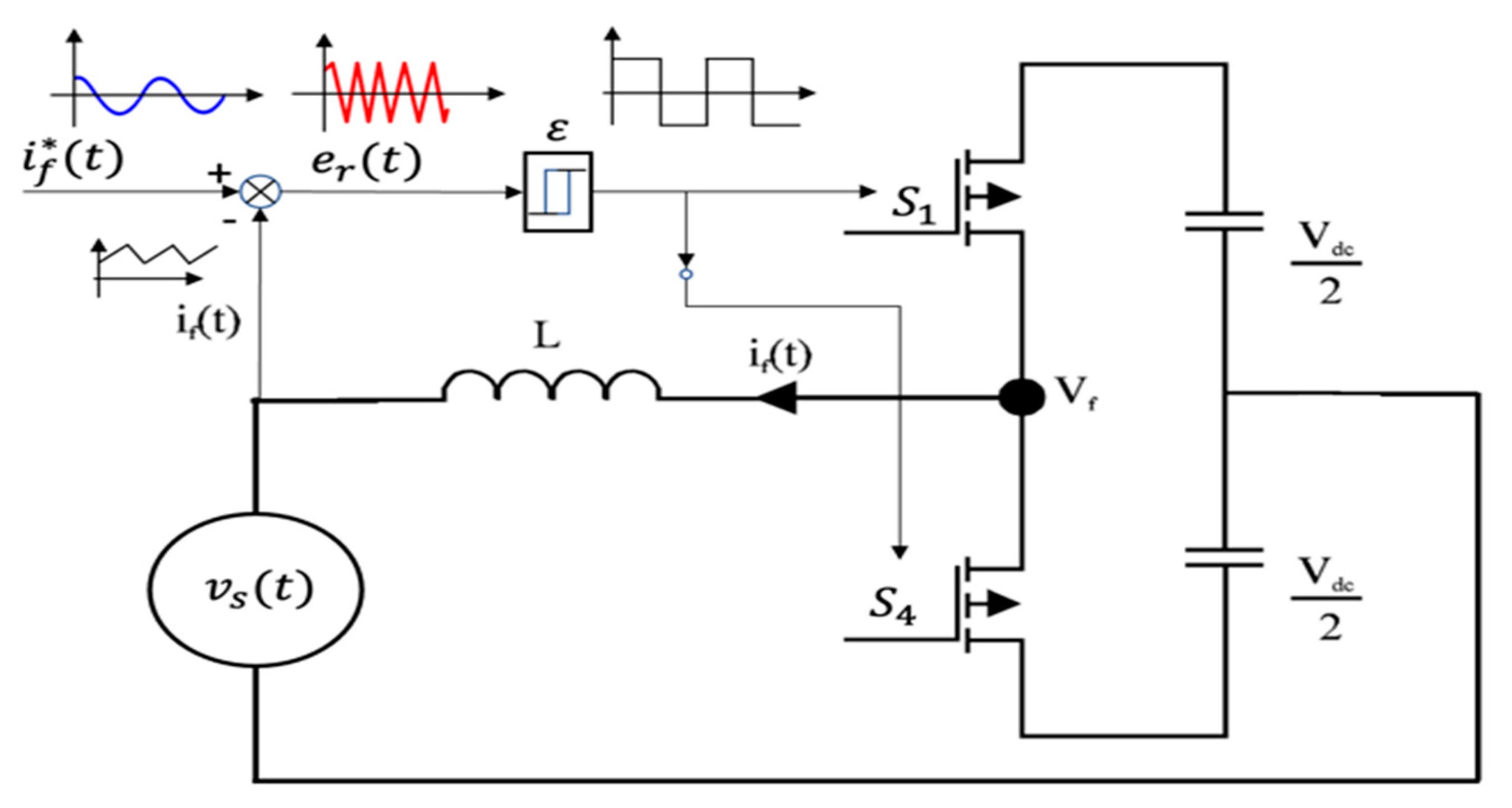
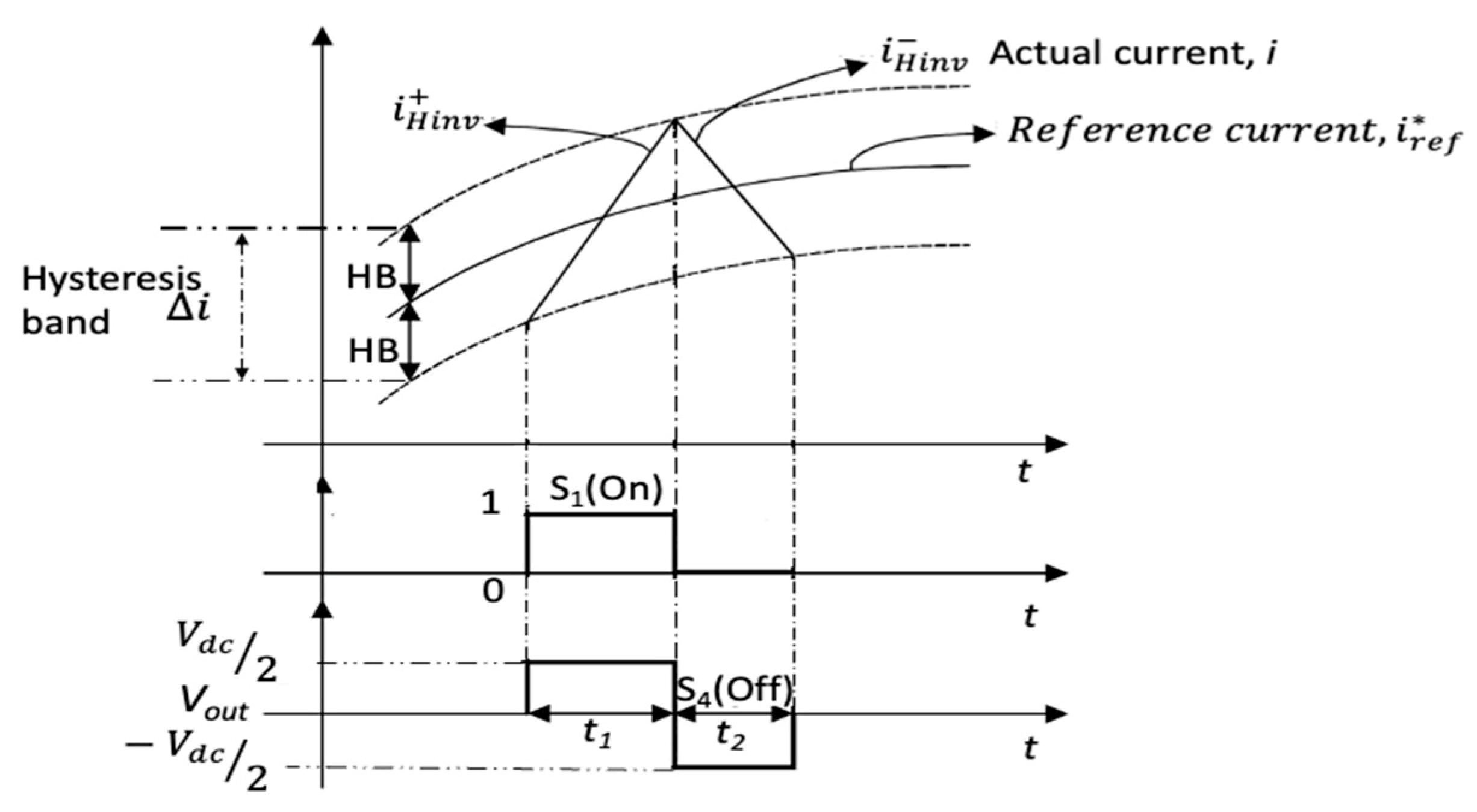
3. The Hysteresis Current Controller

The implementation of the traditional constant bandwidth variable frequency HCC (CBVF-HCC) involves comparing the reference current to the inverter current within the hysteresis band, as seen in Figure 2. The aim is to obtain an error current, er(t), as minimum as possible within a hysteresis bandwidth and generate an appropriate gating signal.
Considering a sinusoidal supply voltage with no harmonics, the inverter voltage, V f , is dependent on the appropriate switching scheme of the inverter switches as well as the modulation index. Under linear modulation mode and considering the current direction in Figure 2, V f can be generalized as:
V f = ( S 1 S 4 ) × V d c 2
For Vc = V d c 2
V f = { V C   f o r   S 1 = 1   V C   f o r   S 4 = 1
Again, from Figure 2, the following expressions can be obtained for the rate of change in the inverter current and that of the reference current, respectively.
d i f ( t ) d t = 1 L ( v f v s ( t ) )
d i f * ( t ) d t = 1 L ( v f * v s ( t ) )
The error current, e r ( t ) , is calculated for each phase of the VSC and obtained from Figure 3, where the inverter current tracks the reference current, within the hysteresis bandwidth, to generate gating pulses for the VSC.
e r ( t ) = [ e r a e r b e r c ] = [ i f a * i f b * i f c * ] [ i f a i f b i f c ]
Δ e r Δ t = 2 ε t 1 = d i f * ( t ) d t d i f ( t ) d t
From Figure 3, the rate of change in the error current can be deduced, for the rising and falling periods, as Equation (14) and Equation (15), respectively. From these, a relation between the hysteresis bandwidth and the switching frequency can be obtained by substituting Equations (14) and (15) into Equation (13).
d i f + ( t ) d t = 1 L ( v f v s ( t ) )
d i f ( t ) d t = 1 L ( v f + v s ( t ) )
{ 2 ε = d i f * ( t ) d t × t 1 d i f + ( t ) d t × t 1 2 ε = d i f * ( t ) d t × t 2 d i f ( t ) d t × t 2
Equation (16) is the traditional relation for obtaining the hysteresis current error, ε . From the expression, a fixed band is obtained, but variable and uncontrollable switching frequencies will be observed. This results in several challenges in using the HCC controller including difficulties in harmonic filter design due to the uncontrollable nature of the switching frequency. This article resolves this issue by presenting a novel equation that expresses the maximum instantaneous switching frequency with respect to the error band current.
The basic condition for the successful implementation of this controller is for the rate of change in the reference current to be smaller than that of the inverter current shown in Equation (16). Equations (17)–(21) calculate the hysteresis current bandwidth as well as present an expression for the instantaneous switching frequency of the VCS for a finite time period, T.
d i f + d t > d i f * d t
t 1 = 2 ε ( d i f + d t d i f * d t )
t 2 = 2 ε ( d i f * d t d i f d t )
If the total period T = t1 + t2, then the frequency can be obtained as Equation (20), and eventually Equation (21) gives the novel expression. The frequency is to be obtained instantaneously for each sampling time and for each phase.
f i n s t = 1 T = 1 t 1 + t 2
f i n s t = 1 2 ε ( 1 1 d i f + d t d i f * d t + 1 d i f * d t d i f d t )
where
i f + ( t ) : rising current;
i f ( t ) : falling current;
i f * : reference current;
f i n s t : inverter switching frequency;
d i f + d t and d i f d t : the rising and falling rate of change in inverter current;
d i f * d t : rate of change in reference current.

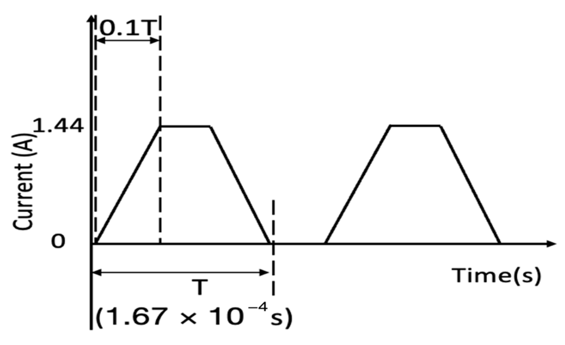
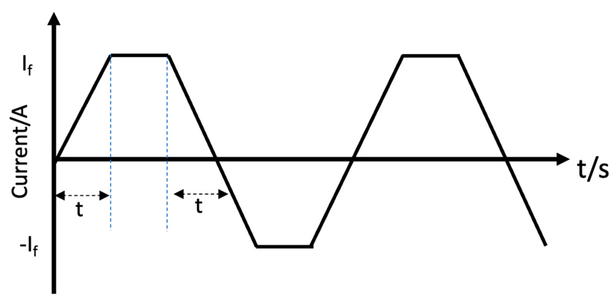
3.1. Validation of the Novel Expression

The obtained expression will work for all load types, constant and varying, provided the principles of hybrid filter designs are followed. Irrespectively, the expression was simulated with three reference signals: sinusoidal, square wave and the trapezoidal reference signals considering a supraharmonic frequencies source from an MC interfaced constant load application, although only the results of the trapezoidal reference signal are presented in this article.
Hybrid active filter topology was selected for the compensation due the fact that passive L-C filter solutions will be too bulky and heavy to be implemented in applications where size and weight are important, which is the major target application considered in this article. Active filters, on the other hand, will be too expensive considering the frequency range. The HAPF consists of a passive filter section and an active power filter section with its controls. The passive side of the HAPF was to meet the following requirements.
  • Filter input impedance at grid frequency must be less than or equal to the grid impedance and higher at harmonic frequencies.
  • Filter current transfer ratio must be low at grid frequency.
The above rules governed the sizing of the passive filter components and resulted in an RLC passive filter selection. The capacitor value was designed based on the reactive power requirements at grid frequency, and the inductor selection was based on the consideration that the voltage drop in the RLC filter must be 5% of the grid voltage. There is a maximum passive filter attenuation of 60% to maintain a smaller size passive filter element. The following equations were used to obtain the passive filter parameters.
| H ( j ω ) | = | 1 1 ( ω S W ω C ) 2 |
C F = K C S M C 3 V s 2 ω g
The filter inductance was calculated after obtaining C F and the cutoff frequency, ω C , using the following equation.
ω C = 1 L F × C F
For the active side of the HAPF, the main components are the DC capacitance voltage and capacitance value and the coupling inductance value. The reactive power produced by the inverter can compensate the reactive power in the supply when the VSC output voltage is higher than the supply voltage; thus, V i n v > V s under linear modulation mode. The DC capacitance voltage, Vdc was obtained as Equation (26) by:
m a = 2 2 V i n v V d c
If m a = 1 , then
V d c = 2 2 V i n v = 2 ( 2 / 3 ) V s
The selection of the DC capacitance value was based on the instantaneous power exchange between the inverter and the grid during transients. The peak-to-peak ripple voltage of the inverter was assumed to be 15% of the DC bus voltage. Hence, the lost energy in the inverter is compensated for as shown in Equation (27):
E = 1 2 C d c ( V 1 2 V 2 2 ) = P × T = K 3 V S I f a T
where V 2 = V 1 Δ V r i p p and Δ V r i p p is the peak-to-peak ripple voltage. V1 is the DC voltage. If the power rating of the inverter is P, then the energy stored in the capacitor for a period T can be estimated.
The selection of the coupling inductor was based on the peak-to-peak ripple current, iripp, which was calculated considering the harmonic currents to be 10% of the input current to the MC.
L 2 3 V d c V s sin ( ω t ) m a x | d i L d t |
Equation (21) expresses the VSC switching frequency in terms of the hysteresis band current, the rate of change in the both the reference current and that of the inverter current. From Equation (21), the maximum allowable HCC can be measured, and a near constant switching frequency can be obtained under supraharmonic applications. The obtained expression was verified in an open-loop control simulation using the trapezoidal reference signal.
The trapezoidal reference signal was considered as it closely represented the speed of change in the MC harmonic currents. Figure 4 shows the simulation for the trapezoidal reference signal. For a harmonic frequency of 6 kHz, the minimum coupling inductance size required for the shunt active filter is calculated from equations based on [39] considering a 1 kW 6 kHz converter coupled to a 400 V 50 Hz supply.
The maximum current change rate of the VSC and the minimum coupling inductance, L, can be calculated based on Figure 5 for a 6 kHz harmonic frequency at t = 90/ ω as Equation (29) using Equation (28).
m a x | d i L d t | = 1.44 0.1 × 1.67 × 10 4 = 86.23 × 10 3   A / s L 2 3 V d c V s sin ( ω t ) m a x | d i L d t | = 466.667 V S 86.23 × 10 3 = 0.77   mH
With Equation (28), the rate of change in the VSC output current can be calculated using Equations (14) and (15) for the rising and falling currents and the RMS value of the supply voltage.
d i f + ( t ) d t = 3.89 × 10 5 A / s                                                   d i f ( t ) d t = 1.43 × 10 6   A / s
For a trapezoidal wave reference current of Figure 6, the rate of change in the reference current, considering the first four terms of a trapezoidal wave equation, can be expressed as Equation (31). The rate of change in the converter current at harmonic frequency of 6 kHz is calculated as Equation (32).
i f * = 8 2 π 2 I f * ( sin ( ω t ) + sin ( 3 ω t ) 9 sin ( 5 ω t ) 25 sin ( 7 ω t ) 49 ) d i f * d t = 8 2 π 2 I f * ω ( 1 + 1 3 1 5 1 7 )
d i f * d t = 6.16 × 10 4   A / s
From Equations (30) and (31), the maximum switching frequency for a trapezoidal wave shape reference current can then be obtained as Equation (33).
f i n s t = 1 2 ε ( 1 1 3.89 × 10 5 6.16 × 10 4 + 1 6.16 × 10 4 + 1.43 × 10 6 ) f i n s t = 131.90 ε kHz
The trapezoidal reference signal by nature closely represents the matrix converter load current shape as seen in Figure 7 and by the above deductions; an instantaneous switching frequency, based on the parameters used, is 131.9 kHz considering a hysteresis band of 1 A.

3.2. Effects of the Power Rating of the MC on Inverter-Switching Frequency

The effects of the MC power rating on the maximum instantaneous switching frequency of the VSC was analyzed with MC ratings of 10 kW, 50 kW and 100 kW. Each had a 6 kHz frequency on the trapezoidal signal, as it closely represented the MC current shape. For the above converter rating, the appropriate MC input current, If, was obtained with Equation (34). For the MC rated capacity, SMC, of 10 kW, the MC input current and the maximum rate of change in the reference current can be obtained from Equations (34) and (35).
I f = S M C 400 3 = 14.43   A
d i f * d t = 8 2 π 2 I f * ω ( 1 + 1 3 1 5 ) = 7.06 × 10 5   A / s
The instantaneous frequency of the VSC can be calculated from Equation (35), and the rate of change in the rising and falling inverter current of Equations (30) and (31) is shown as Equation (36).
d i f + ( t ) d t = ( 700 400 ) 0.077 m H = 3.88 × 10 6   A / s d i f ( t ) d t = ( 700 + 400 ) 0.77 m H = 1.47 × 10 7   A / s f i n s t = 1 2 ε ( 1 1 3.89 × 10 6 7.06 × 10 5 + 1 7.06 × 10 5 + 1.47 × 10 7 ) f i n s t = 1.319 ε M H z
Table 3 summarizes the deduction above with a different matrix converter power, SMC at 6 kHz, which is expressed as a ratio of the hysteresis band current. From the table, it can be concluded that the VSC switching frequency is directly proportional to the power of the MC. Hence, an increment in the MC power increases the VSC switching frequency, which proves the theory.
Finally, the effects of the hysteresis current error, ε , and the maximum instantaneous switching frequency are analyzed. From Equation (21), the relation between ε and f i n s t is inversely proportional. The error current was toggled between 0.2 A, 0.5 A, 0.7 A and 1 A at 10 kW MC rated power. Table 4 shows the obtained results.

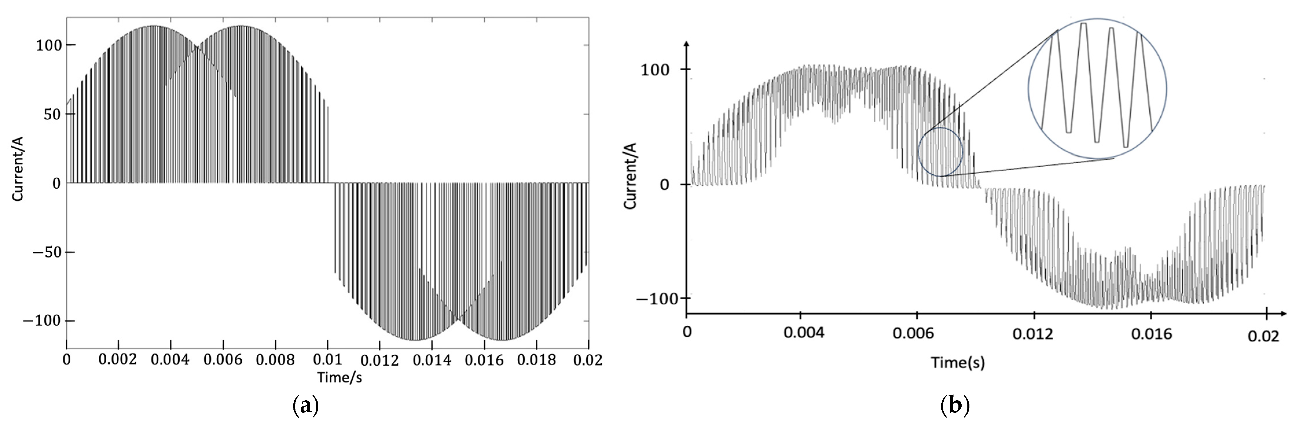
4. Simulation Results and Analysis

A simulation of the theory was first conducted in a three-phase, open-loop configuration for the trapezoidal reference signal. A closed-loop simulation of a hybrid active filter for an MC interfaced three-phase load was analyzed. Figure 8 depicts a three-phase voltage source supplying a three-phase MC interfaced load. The HAPF consisted of the parallel combination of a shunt active power filter (SAPF) and a passive L-C filter. Table 5 shows the parameters selected for the simulations of the MC-HAPF in MATLAB/Simulink environment based on equations from an earlier work by the same authors [39]. Irrespectively, non-ideal conditions were included in the simulation to approximate practical implementation for future work.
The open-loop setup consisted of a three-phase supply and the MC coupled load as seen in Figure 4 above. The open-loop reference trapezoidal signal was compared to the VSC output current signal in the presence of the hysteresis band. The trapezoidal signal was selected because its rate of change in current closely mimics that of the matrix converters. Table 6 shows the parameters for the trapezoidal reference simulation. The effects of the reference signal’s frequency and hysteresis current bandwidth on the switching frequency of the VSC were tabulated and analyzed.
The simulation results for the open-loop and closed-loop configurations are shown below. The open-loop current shape and its maximum switching frequency as well as that for the closed-loop hysteresis-controlled MC setup are shown in Figure 9 and Figure 10, respectively.

5. Discussion

From Table 7, it was observed that the simulation results followed the calculated results. Also, the results obtained from the MC-HAPF showed a 600 kHz maximum HAPF switching frequency for a 50 kW MC with 6 kHz switching frequency. The implementation of the above active part of the hybrid filter will involve the use of high-switching transistors. An example will be paralleling two IPW60R120P7 or R6030KNZ4 power MOSFETS for this purpose. Insulated gate bipolar transistors, IGBT’s, are the most used transistors for inverter design for low frequencies (20 to 100) kHz and higher power applications, while metal–oxide–semiconductor field effect transistors, MOSFETs, are most suitable for low power and higher frequency (in MHz) range applications. However, there is the possibility of paralleling power MOSFETs for high power and frequency applications. From the above simulations, the following deductions were observed:
  • The converter rated power is directly proportional to the maximum attainable active filter hysteresis switching frequency.
  • Again, the maximum hysteresis switching frequency increases with the decrease in the hysteresis bandwidth current.
  • Reference signals with rate of change close to the supraharmonic signal frequency reduces the maximum hysteresis switching frequency of the VSC.
With these observations, the following recommendations are suggested. For higher-frequency applications (6–10 kHz), power MOSFETs are recommended for hysteresis active filter-switching applications. However, to prevent switching loses, it is recommended to maintain a converter rated power below 50 kW. In applications with higher power (above 50 kW) and relatively lower converter switching frequencies (below 6 kHz), IGBTs are recommended. IGBTs are not recommended for higher frequency applications but are most recommended for lower switching frequency converters. Also, for EMI and oscillations control, the gate resistor of MOSFETS, irrespective of the connected load, needs to be carefully selected as the size of the gate resistors mostly affects the switching frequency of the power MOSFET. Table 8 shows an IGBT and MOSFET data sheet from Infineon and the ST catalog. Further information about the MOSFET switching frequencies is provided in Appendix A.
The harmonic distribution of the MC coupled load was analyzed, and Table 9 shows the MC input current harmonic distribution obtained after the simulation without any filter, passive or hybrid, at a sampling time of 4 × 10 7 with 50,000 samples per cycle. Without any filter, fast Fourier transform analysis (FFT) of the input current shows the total harmonic distortion of 57.49%, as seen in Figure 11a, with the dominant higher frequency harmonics occurring at the 155th harmonic level, which is close to the MC switching frequency. This further proved the influence of the switching frequency of the MC on the grid.
The introduction of the passive L-C filter, as the interface to the MC, reduced the THD of the MC input current to 20.82% with the dominant h155 harmonic reducing to 10% of the fundamental. The passive filter could be designed to achieve more attenuation, but this will increase the size and weight of the filter as well as the reactive power burden and possibly lead to resonance conditions. Figure 11b shows the FFT analysis of the input current when a passive L-C filter was employed.
The implementation of the SAPF as the only filter interface between the MC input current and the supply grid resulted in a THD of 20.84% with h155 as 0.63% from FFT analysis. The SAPF could not achieve further compensation, as a large compensational current must be supplied by the SAPF. The hysteresis current controller maintained a constant switching frequency of 80 kHz for the inverter gating pulses. Figure 11c shows the THD of the MC input current in the FFT window.
The introduction of the HAPF resulted in the overall increase in the RMS value of the fundamental current to 91.8 A. While the passive part of the HAPF attenuated the supraharmonics, the active part of the HAPF compensated the lower frequency harmonics. By this principle, better harmonic compensation was achieved. At the same sampling time and samples per cycle, the THD of the input current under the HAPF was successfully reduced to 2.31%, and the h155 harmonic level compensated to 0.16% of the fundamental 50 Hz. These are within the IEEE Std. 519-2022 standards. Figure 11d shows the FFT analysis of the MC input current when the HAPF was used.

6. Conclusions

Supraharmonics in the power system affects power quality and affects load parameters. Traditional passive and active filters may not be enough to compensate these high-frequency harmonics. This investigation provides filter designers with enough information about the strengths and weaknesses regarding the use of HCCs for active power filters. The obtained novel equation debunks the popular notion of uncontrollable and variable switching frequencies, difficulty in filter design and higher loses associated with HCCs when used as higher frequency inverter current controls. The novel equation can be used to size inverters for any application. As controller for active filters, the HAPF achieved 0.16% THD of the dominant h155 harmonic level after implementation. Compared to traditional passive filter solutions, the obtained results present a better option for MC high-input current harmonic attenuation, as the size and weight of the filter is much improved. The limitations proposed by [39] pertaining to the crippling of the switching frequency by the HCC have been overcome. Future research is directed toward optimization of the equation and the use of model predictive controllers.

Author Contributions

Conceptualization, G.S.; methodology, G.S. and A.K.; software, A.K., A.B. and S.O.F.; validation, G.S., A.B., S.O.F. and A.K.; formal analysis, G.S.; investigation, G.S., A.B., S.O.F. and A.K.; resources, G.S. and A.K.; writing—original draft preparation, A.K.; writing—review and editing, G.S. and A.K.; visualization, G.S. All authors have read and agreed to the published version of the manuscript.

Funding

This research received no external funding.

Institutional Review Board Statement

Not applicable.

Informed Consent Statement

Not applicable.

Data Availability Statement

Data contained within the article.

Conflicts of Interest

The authors declare no conflicts of interest.

Nomenclature

C D C DC link capacitance
C f Passive filter capacitance
C H f HAPF passive-side capacitance
HAPFHybrid active power filter
IMCMatrix converter current at grid frequency
ISSource current
L f Passive filter inductance
L H f HAPF passive-side inductance
L_C/L_HinvSAPF/HAPF coupling inductance
MCMatrix converter
SAPFShunt active power filter
SMCRated power of matrix converter
VSSource voltage
VSCVoltage source converter
ω Base frequency in radian
ω C Resonance frequency in radian

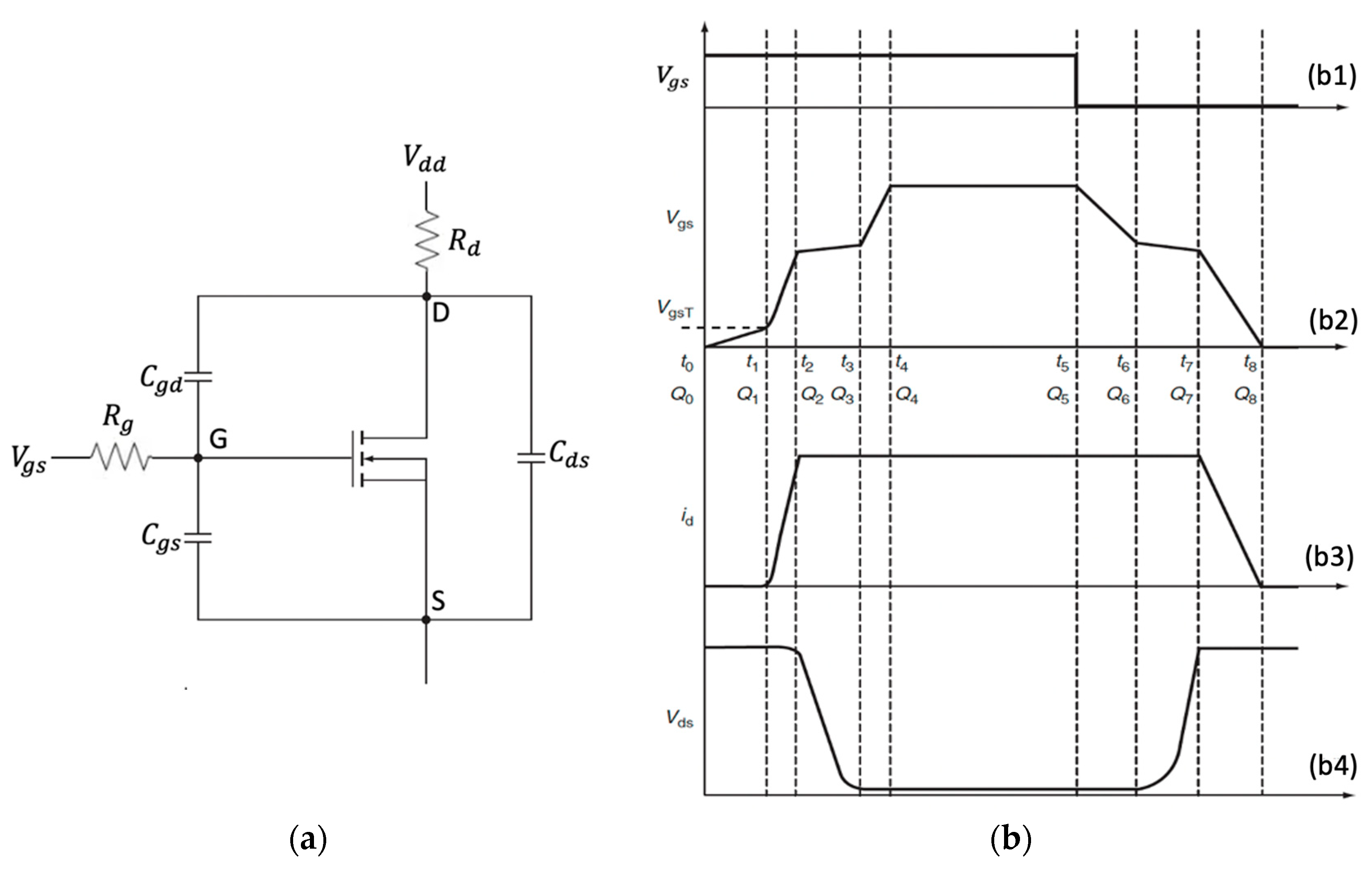
Appendix A. Effects of the VSC Switches on Maximum Switching Frequency

MOSFETS are widely used in applications that require higher power density and efficiency due to their higher switching speeds and lower losses [38,39]. Irrespectively, increasing the switching speed naturally induces oscillations, higher frequency harmonics, voltage and current overshoots and even more loses. This challenges the use of the MOSFET in power converters, VSCs and active harmonic filters under supraharmonic frequency applications.
The power MOSFET can be modeled as in Figure A1a which shows the parasitic capacitors; gate-to-source capacitor, Cgs, gate-to-drain capacitor, Cgd, and drain-to-source capacitor, Cds of a power MOSFET. The gate of the MOSFET is insulated from the substrate; hence, an initial gate current, Ig, is needed to charge both Cgs and Cgd to turn on the MOSFET. To turn off the MOSFET, the gate drive must be bi-directional to conduct/sink current away from the gate [40,41,42,43,44].
From Figure A1 and considering the initial switching-on stage, the parasitic input capacitances, (Cgs + Cgd), are charged through the gate resistor, Rg, for a period of t0 +t1 = T1. The total time delay is dependent on the input capacitance and the logarithmic function of the gate voltage and its threshold. This can be expressed as shown in Equation (A1).
T 1 R g ( C g s + C g d ) ln ( V g s V g s V g s T )
The second stage requires raising Vgs above the miller plateau. At this stage, the transistor is unblocked and experiences feedback from Cgd. The drain voltage drops to its minimum as the drain current increases to its maximum. The total charge, Qtot3, and the equivalent charge, Ceq, required through this stage are estimated as Equation (A2) and Equation (A3), respectively. The total delay can be estimated as T2 in Equation (A5) [45].
Figure A1. (a) Parasitic capacitance model of the power MOSFET; (b) switching characteristics of a power MOSFET. Cgd: Gate to drain capacitance; Cgs: Gate to source capacitance; Cds: Drain to source capacitance; D: Drain; G: Gate; Rg: Gate resistance; Rd: Load resistance; S: Source; V g s : Gate-to-source voltage; V d d : Transistor voltage source; Q(1-8): Capacitance charge; V g s T : Gate-to-source threshold voltage; V d s : Drain-to-source voltage; Vdsmin: Minimum drain voltage.
Applsci 14 01713 g0a1
Q t o t 3 = V g s C g s + C g d ( V g s + V d d )
C e q = Q t o t 3 V g s m a x = C g s + C g d ( 1 + V d d V g s m a x )
V d d V g s m a x = m i l l e r   e f f e c t
T 2 0.8 C g d R g ( V d d V d s m i n ) V g s V gsT ( V d d + V d s m i n ) / 2 R d S
For S :   Δ I d / Δ V g s
In the third stage, the Vds drops to its minimum, and the MOSFET is driven in full enhancement mode, and the total time duration is T3 in Equation (A6).
T 3 3 R g ( C gs + C g d )
T1+ T2+ T3 makes up the total turn on time of the MOSFET, Ton.
T o n = T 1 + T 2 + T 3 T o n = 1.6 C g d R g R d V d d S 2 V g s R d S V g s T V d d + R g ( 3 + ln ( V g s V g s V g s T ) ) ( C g s + C g d )
At
V d s m i n 0
The total required gate current to turn on the MOSFET can be calculated as shown in Equation (A8).
i g = C e q V g s m a x T o n
The next stage is from t4–t5, which is characterized by constant values of currents and voltages and equivalent to the saturation stage of a bipolar transistor. The gate current remains zero during t4t5 when the MOSFET is fully on. No charge is required to keep it on.
The fifth stage begins the turn-off stage of the MOSFET. The gate pulse signal becomes zero, and the turn-off sequence is initiated. When the input pulse signal drops to zero, the capacitance C g s + C g d begins to be discharged. It is most important for the appropriate gate driver to be bi-directional. The total time required to discharge can be calculated as Equation (A9).
T 4 = R g ( C gs + C g d ) ln ( V g s V d i s s )
where the discharge voltage is given as Equation (A10).
V d i s s = V g s T + ( V d d V d s m i n ) R d S
The MOSFET is discharged from the ohmic region to the off state. The drain-to-source voltage is increased during this time. The total time duration can be given by Equation (A11).
T 5 0.8 C g d R g ( V d d V d s m i n ) V gsT + ( V d d V d s m i n ) / 2 R d S
In the final stage, Cgs is discharged to a full turn-off state, Vds is raised to its initial value and Id is minimized to zero. The total time delay can be estimated based on Rg and the input capacitances as in Equation (A12).
T 6 3 R g ( C gs + C g d )
The total off time can be estimated based on the combination of T4 + T5 + T6 as in Equation (A13) at a minimum Vdsmin of 0.
T o f f = 1.6 C g d R g R d V d d S 2 V g s T R d S + V d d + R g ( 3 + ln ( V g s V g s m a x ) ) ( C g s + C g d )
The total switching time of the MOSFET can be calculated as Ton + Toff. The maximum allowable switching frequency based on the above deduction can then be obtained with the inverse of the total switching period. Considering the IRFP450 enhancement mode MOSFET parameters specified in Table A1, the total on and off time delays from Equations (A7) and (A13), the maximum switching frequency can be mathematically estimated as Equation (A14).
Table A1. IRFP450 MOSFET parameters.
ParameterValue
Vdd500 V
Drain-to-source voltage, Vds500 V
Drain current, Id14 A
Gate-to-source voltage, ± Vgs20 V
Ciss (Cgs + Cgd)2600 pF
Coss (Cds + Cgd)720 pF
Crss/Cgd340 pF
Cgs2260 pF
Cds380 pF
Conductance, S1–10 mA/V
Gate-to-source threshold voltage, (VgsT)2–4 V
T o n = 2.72 × 10 7 R g R d S 40 R d S 1500 + 8.22 × 10 9 R g
T o f f = 2.72 × 10 7 R g R d S 6 R d S + 50 + 7.8 × 10 9 R g
For
S: 1 mA/V
Rg: 3 Ω Rd: 3.57 Ω
T t o t = 8.16 × 10 7 0.12 1500 + 8.16 × 10 7 0.018 + 500 + 4.8 × 10 8 F s w = 1 T o n + T o f f = 20.8 M H z
The obtained maximum frequency, Fsw, from Equation (A14) is calculated based on manufacturers data provided on the datasheet of the IRFP450, and operational values will differ. The maximum obtainable frequency was analyzed for various values of Rg and Rd at S = 1 mA/V. Table A2 and Table A3 show the results of these variations of the frequency. From Table A3, it can be observed that increasing the gate resistance alleviates the switching frequency, which will eventually reduce oscillations and electromagnetic interferences (EMIs) [44,45,46,47]. However, the reduction in switching speed increases switching losses and the on/off time delays.
Table A2. Maximum switching frequency at constant gate resistance, Rg (3 Ω ) and variable load resistance, Rd.
ParameterValue
RdFull load resistance (3 Ω )10 k Ω 100 k Ω 300 k Ω
Fsw20.8 MHz18.1 MHz6.4 MHz5.6 MHz
Table A3. Maximum switching frequency at constant gate resistance, Rd (3.57 Ω) and variable gate resistance, Rg.
ParameterValue
Rg1 Ω 3 Ω 10 Ω 20 Ω
Fsw62.4 MHz20.8 MHz6.2 MHz3.12 MHz

References

  1. Slangen, T.; van Wijk, T.; Ćuk, V.; Cobben, S. The Propagation and Interaction of Supraharmonics from Electric Vehicle Chargers in a Low-Voltage Grid. Energies 2020, 13, 3865. [Google Scholar] [CrossRef]
  2. Yanchenko, S.; Meyer, J. Impact of Network Conditions on the Harmonic Performance of PV Inverters. In Proceedings of the 2018 Power Systems Computation Conference (PSCC), Dublin, Ireland, 11–15 June 2018; pp. 1–7. [Google Scholar] [CrossRef]
  3. Moreno-Munoz, A.; Gil-de-Castro, A.; Rönnberg, S. Ongoing work in cigre working groups on supraharmonics from power-electronic converters. In Proceedings of the 23rd International Conference on Electricity Distribution, Lyon, France, 15–18 June 2015; p. 5. [Google Scholar]
  4. Pugliese, S.; Flacke, S.; Zou, Z.; Liserre, M. High-Frequency Harmonic Current Control of Power Converters. In Proceedings of the 2019 IEEE Energy Conversion Congress and Exposition (ECCE), Baltimore, MD, USA, 29 September–3 October 2019; pp. 6915–6921. [Google Scholar] [CrossRef]
  5. Thomas, T.; Michael, P.A. A review of high frequency emission in 2–150 kHz range. Int. J. Adv. Appl. Sci. 2020, 9, 132–141. [Google Scholar] [CrossRef]
  6. Alfalahi, S.T.Y.; Alkahtani, A.A.; Al-Shetwi, A.Q.; Al-Ogaili, A.S.; Abbood, A.A.; Bin Mansor, M.; Fazea, Y. Supraharmonics in Power Grid: Identification, Standards, and Measurement Techniques. IEEE Access 2021, 9, 103677–103690. [Google Scholar] [CrossRef]
  7. Zhang, C.; Cao, C.; Chen, R.; Jiang, J. Three-Leg Quasi-Z-Source Inverter with Input Ripple Suppression for Renewable Energy Application. Energies 2023, 16, 4393. [Google Scholar] [CrossRef]
  8. Wang, J.; Fang, Y.; Fei, J. Adaptive Super-Twisting Sliding Mode Control of Active Power Filter Using Interval Type-2-Fuzzy Neural Networks. Mathematics 2023, 11, 2785. [Google Scholar] [CrossRef]
  9. Liu, T.-H.; Li, J.-H. Design and Implementation of Input AC Filters and Predictive Control for Matrix-Converter Based PMSM Drive Systems. Energies 2022, 15, 748. [Google Scholar] [CrossRef]
  10. Jajarmi, H.R.I.; Mohamed, A.; Shareef, H.; Subiyanto. Adaptive interval type2 fuzzy hysteresis-band current-controlled active power filter for power quality improvement owe. Prz. Elektrotechniczny 2014, 90, 140–145. [Google Scholar] [CrossRef]
  11. Schneider Electric, “Variable Speed Drives Altivar61 for asynchronous motors,” Catalogue. 2014. Available online: https://inverterdrive.com/file/Schneider-Altistart-01-Catalogue-2014 (accessed on 14 February 2024).
  12. Koduah, A.; Svinkunas, G. Switching Harmonic Ripple Attenuation in a Matrix Converter-Based DFIG Application. In Proceedings of the 2022 IEEE 7th International Energy Conference, Riga, Latvia, 9–12 May 2022; pp. 1–7. [Google Scholar] [CrossRef]
  13. Dwivedi, A.; Tiwari, A. Analysis of three-phase PWM rectifiers using hysteresis current control techniques: A survey. Int. J. Power Electron. 2017, 8, 349. [Google Scholar] [CrossRef]
  14. Durna, E. Adaptive fuzzy hysteresis band current control for reducing switching losses of hybrid active power filter. IET Power Electron. 2018, 11, 937–944. [Google Scholar] [CrossRef]
  15. Albanna, A.Z.; Hatziadoniu, C.J. Harmonic Modeling of Hysteresis Inverters in Frequency Domain. IEEE Trans. Power Electron. 2009, 25, 1110–1114. [Google Scholar] [CrossRef]
  16. Albanna, A. Modeling & Simulation of Hysteresis Current Controlled Inverters Using MATLAB. In Applications of MATLAB in Science and Engineering; Michalowski, T., Ed.; IntechOpen: London, UK, 2011. [Google Scholar] [CrossRef]
  17. IEEE Std 519-2022; IEEE Standard for Harmonic Control in Electric Power Systems. Institute of Electrical and Electronics Engineers: New York, NY, USA, 2022. [CrossRef]
  18. Wang, Y.; Luo, D.; Xiao, X. Evaluation of supraharmonic emission levels of multiple grid-connected VSCs. IET Gener. Transm. Distrib. 2019, 13, 5597–5604. [Google Scholar] [CrossRef]
  19. Meyer, J.; Haehle, S.; Schegner, P. Impact of higher frequency emission above 2 kHz on electronic mass-market equipment. In Proceedings of the 22nd International Conference and Exhibition on Electricity Distribution (CIRED 2013), Stockholm, Sweden, 10–13 June 2013; p. 0999. [Google Scholar] [CrossRef]
  20. Klatt, M.; Stiegler, R.; Meyer, J.; Schegner, P. Generic frequency-domain model for the emission of PWM-based power converters in the frequency range from 2 to 150 kHz. IET Gener. Transm. Distrib. 2019, 13, 5478–5486. [Google Scholar] [CrossRef]
  21. Chiang, G.T.; Itoh, J.-I. Voltage transfer ratio improvement of an Indirect Matrix Converter by Single pulse modulation. In Proceedings of the 2010 IEEE Energy Conversion Congress and Exposition (ECCE), Atlanta, GA, USA, 12–16 September 2010; p. 9. [Google Scholar] [CrossRef]
  22. Karpagam, J.; Kumar, N.; Kumar, C. Comparison of Modulation Techniques for Matrix Converter. Int. J. Eng. Technol. 2010, 2, 189. [Google Scholar]
  23. Monteiro, J.; Pinto, S.; Martin, A.D.; Silva, J.F. A New Real Time Lyapunov Based Controller for Power Quality Improvement in Unified Power Flow Controllers Using Direct Matrix Converters. Energies 2017, 10, 779. [Google Scholar] [CrossRef]
  24. Li, D.; Wang, T.; Pan, W.; Ding, X.; Gong, J. A comprehensive review of improving power quality using active power filters. Electr. Power Syst. Res. 2021, 199, 107389. [Google Scholar] [CrossRef]
  25. Goel, S.; Tiwari, D.; Pandey, M.K.; Bajpai, S. Power Quality Conditioners for Matrix Converter Using Shunt and Series Active Filters. Int. J. Electron. Electr. Eng. 2013, 6, 119–130. [Google Scholar]
  26. Dabour, S.M.; Rashad, E.M. Improvement of Voltage Transfer Ratio of Space Vector Modulated Three-Phase Matrix Converter. In Proceedings of the IEEE 15th International Middle East Power Systems Conference (MEPCON’12), Alexandria, Egypt, 23–25 December 2012; pp. 581–586. [Google Scholar]
  27. Koduah, A.; Svinkunas, G.; Ampofo, D.O. Design of a Shunt Active Power Filter for Direct Matrix Converter Application. In Proceedings of the 2021 IEEE PES/IAS PowerAfrica, Nairobi, Kenya, 23–27 August 2021; pp. 1–5. [Google Scholar] [CrossRef]
  28. Praženica, M.; Kaščák, S.; Resutík, P. Power Losses Investigation in Direct 3 × 5 Matrix Converter Using MATLAB Simulink. Appl. Sci. 2023, 13, 4049. [Google Scholar] [CrossRef]
  29. Toledo, S.; Caballero, D.; Maqueda, E.; Cáceres, J.J.; Rivera, M.; Gregor, R.; Wheeler, P. Predictive Control Applied to Matrix Converters: A Systematic Literature Review. Energies 2022, 15, 7801. [Google Scholar] [CrossRef]
  30. Janabi, A.; Wang, B. Hybrid matrix converter based on instantaneous reactive power theory. In Proceedings of the IECON 2015—41st Annual Conference of the IEEE Industrial Electronics Society, Yokohama, Japan, 9–12 November 2015; pp. 003910–003915. [Google Scholar] [CrossRef]
  31. El-Habrouk, M.; Darwish, M.; Mehta, P. Active power filters: A review. IEE Proc. Electr. Power Appl. 2000, 147, 403–413. [Google Scholar] [CrossRef]
  32. Büyük, M.; Tan, A.; Tümay, M.; Bayındır, K. Topologies, generalized designs, passive and active damping methods of switching ripple filters for voltage source inverter: A comprehensive review. Renew. Sustain. Energy Rev. 2016, 62, 46–69. [Google Scholar] [CrossRef]
  33. Akagi, H.; Watanabe, E.H.; Aredes, M. Instantaneous Power Theory and Applications to Power Conditioning, 2nd ed.; IEEE Press Series on Power Engineering; IEEE Press/Wiley: Hoboken, NJ, USA, 2007. [Google Scholar]
  34. Watanabe, E.H.; Aredes, M.; Afonso, J.L.; Pinto, J.G.; Monteiro, L.F.C.; Akagi, H. Instantaneous p–q power theory for control of compensators in micro-grids. In Proceedings of the 2010 International School on Nonsinusoidal Currents and Compensation (ISNCC), Lagow, Poland, 15–18 June 2010; p. 11. [Google Scholar]
  35. Liu, F.; Maswood, A.I. A Novel Variable Hysteresis Band Current Control of Three-Phase Three-Level Unity PF Rectifier with Constant Switching Frequency. IEEE Trans. Power Electron. 2006, 21, 1727–1734. [Google Scholar] [CrossRef]
  36. Singh, J.K.; Behera, R.K. Hysteresis Current Controllers for Grid Connected Inverter: Review and Experimental Implementation. In Proceedings of the 2018 IEEE International Conference on Power Electronics, Drives and Energy Systems (PEDES), Chennai, India, 18–21 December 2018; pp. 1–6. [Google Scholar] [CrossRef]
  37. Vahedi, H.; Sheikholeslami, A.; Bina, M.T. A novel hysteresis bandwidth (NHB) calculation to fix the switching frequency employed in active power filter. In Proceedings of the 2011 IEEE Applied Power Electronics Colloquium (IAPEC), Johor Bahru, Malaysia, 18–19 April 2011; pp. 155–158. [Google Scholar] [CrossRef]
  38. Moran, L.; Dixon, J.; Wallace, R. A three-phase active power filter operating with fixed switching frequency for reactive power and current harmonic compensation. IEEE Trans. Ind. Electron. 1995, 42, 402–408. [Google Scholar] [CrossRef]
  39. Koduah, A.; Effah, F.B. Fuzzy-Logic-Controlled Hybrid Active Filter for Matrix Converter Input Current Harmonics. Energies 2022, 15, 7640. [Google Scholar] [CrossRef]
  40. Tan, J.; Zhou, Z. An Optimized Switching Strategy Based on Gate Drivers with Variable Voltage to Improve the Switching Performance of SiC MOSFET Modules. Energies 2023, 16, 5984. [Google Scholar] [CrossRef]
  41. Dalal, D.N.; Christensen, N.; Jorgensen, A.B.; Jorgensen, J.K.; Beczkowski, S.; Munk-Nielsen, S.; Uhrenfeldt, C. Impact of Power Module Parasitic Capacitances on Medium-Voltage SiC MOSFETs Switching Transients. IEEE J. Emerg. Sel. Top. Power Electron. 2020, 8, 298–310. [Google Scholar] [CrossRef]
  42. Bernacki, K.; Rymarski, Z. The Experimentally Measured Influence of the Si-MOSFET Replacement Switches to WBG Transistors in the Voltage Source Inverters as the Source of Radiation Noise. Energies 2023, 16, 870. [Google Scholar] [CrossRef]
  43. Choi, C.-W.; So, J.-H.; Ko, J.-S.; Kim, D.-K. Influence Analysis of SiC MOSFET’s Parasitic Capacitance on DAB Converter Output. Electronics 2022, 12, 182. [Google Scholar] [CrossRef]
  44. Geng, C.; Zhang, D.; Wu, X.; Shen, W.; Dong, R. A Novel Active Gate Driver with Auxiliary Gate Current Control Circuit for Improving Switching Performance of High-Power SiC MOSFET Modules. In Proceedings of the 2020 IEEE 1st China International Youth Conference on Electrical Engineering (CIYCEE), Wuhan, China, 1–4 November 2020; pp. 1–7. [Google Scholar] [CrossRef]
  45. Yang, Y.; Wen, Y.; Gao, Y. A Novel Active Gate Driver for Improving Switching Performance of High-Power SiC MOSFET Modules. IEEE Trans. Power Electron. 2018, 34, 7775–7787. [Google Scholar] [CrossRef]
  46. Rujas, A.; López, V.M.; Mir, L.; Nieva, T. Gate driver for high power SiC modules: Design considerations, development and experimental validation. IET Power Electron. 2018, 11, 977–983. [Google Scholar] [CrossRef]
  47. Sergeevich, B.S. Circuit Design of Functional Unis of Secondary Power Supply Sources; Handbook; Moscow Radio and Communication: Moscow, Russia, 1992; pp. 72–76. ISBN 5-256-00433-6. [Google Scholar]
Figure 1. Power system with MC interfaced load and hybrid active power filter in between.
Applsci 14 01713 g001
Figure 2. Per phase equivalent of Figure 1 using CBVF HCC. v s ( t ) : supply voltage; i f ( t ) : inverter current; i f * ( t ) : reference current; ε : hysteresis band current; e r ( t ): error current; S 1 , S 4 power inverter switches.
Applsci 14 01713 g002
Figure 3. Hysteresis current control bandwidth gate pulses. i r e f * : Reference current; i H i n v + : Rising inverter current; i H i n v : Falling inverter current; Δ i /HB: Hysteresis current bandwidth; S 1 / S 4 : VSC switch 1 and 4; V o u t : VSC output voltage; V d c : VSC Capacitor voltage.
Applsci 14 01713 g003
Figure 4. Open-loop schematic diagram of HCC-HAPF for MC input current harmonics elimination. Source: [39].
Applsci 14 01713 g004
Figure 5. Maximum rate of change in the harmonic load current. Source: [37]. T: total period in seconds; If: current in amperes.
Applsci 14 01713 g005
Figure 6. Trapezoidal wave shape reference current. t: rising and falling time in seconds; If: current in amperes.
Applsci 14 01713 g006
Figure 7. MC output current shape at 1 kHz switching frequency: (a) unfiltered; (b) with 60% passive L-C filter attenuation.
Applsci 14 01713 g007
Figure 8. Schematic diagram of closed-loop active filter schematic diagram. Source: [39].
Applsci 14 01713 g008
Figure 9. HCC simulation results for reference tracking, error current and maximum-switching frequency for trapezoidal wave reference signal.
Applsci 14 01713 g009
Figure 10. MC-HCC simulation results.
Applsci 14 01713 g010
Figure 11. FFT analysis of MC input current (a) without filter, (b) passive L-C filter only, (c) with SAPF only, (d) with HAPF.
Applsci 14 01713 g011aApplsci 14 01713 g011b
Table 1. Operating frequency ranges of electronic converters for selected loads.
LoadSwitching Frequency (kHz)
Electric vehicle chargers15–100
Solar PV inverters4–20
Power communication lines (PCLs)9–95
Communication notch oscillationsUp to 10
Industrial size converters9–150
Street lighting systemsUp to 20
Household electronic devices (LEDs and CFLs)2–150
Table 2. Similar works review.
ReferencesMethodConclusion
[1]Supraharmonics in electric vehiclesFrequency beating, tripping of residual devices
[3,6,17]Measurement and standardizationsReduces life expectancy of electrical equipment
[16]Supraharmonics in multiple VSCsSupraharmonics are distributed integer multiple of the switching frequency of VSC
[4,5]Supraharmonics in power electronic loads and mode of compensationPower converters are sources of supraharmonics. Zone-phase compensation
[18]Modelling of EMI from supraharmonic devicesIt is possible to model the effects of supraharmonics
[21,22,23]Power quality issues with MC and possible solution with active power filters (APF)Lyapunov control strategy, APF, Shunt and series power filters
[24,25,26,27,29]Supraharmonics in MCLarge switching states of MC causes supraharmonics
Table 3. Effects of changing MC power, SMC, on the converter switching frequency.
SMC/kW/6 kHz11050100
d i f * ( t ) d t , A/s7.06 × 10 4 7.06 × 10 5 3.53 × 10 6 7.06 × 10 6
d i f + ( t ) d t , A/s 3.89 × 10 5 3.89 × 10 6 1.94 × 10 7 3.89 × 10 7
d i f ( t ) d t , A/s 1.47 × 10 6 1.47 × 10 7 7.47 × 10 6 14.29 × 10 8
f i n s t , MHz 0.1319 ε 1.319 ε 6.72 ε 13.19 ε
Table 4. Relationship between hysteresis error current and the VSC switching frequency at SMC (10 kW).
SMC/kW/6 kHz10
ε /A0.2 0.5 0.7 1
f i n s t / M H z 6.722.68 1.921.319
Table 5. Parameters selected for the open-loop configurations.
ParameterValue
Supply voltage (VL-L)400 V, 50 Hz
MC rated power, SMC50 kW
MC switching frequency6 kHz
LC low-pass filter values, CHF33 µF
Passive filter inductance, LHF1.87 mH
Damping resistance, RHF 1   Ω
DC reference voltages653 Vmin, 700 Vmax
DC capacitance100 µF
Coupling inductance115 µH
Table 6. Parameters selected for the closed-loop configurations.
ParameterValue
Supply voltage (VL-L)400 V, 50 Hz
MC rated power, SMC50 kW
MC switching frequency6 kHz
DC capacitor voltage653 Vmin, 700 Vmax
Coupling inductance115 µH
Reference signal frequency50 Hz, 6 kHz
Table 7. Simulation results at hysteresis error current of 1 A.
Novel EquationSimulation Results
MC power, SMC1 kW10 kW1 kW10 kW
Current ref, I f /A1.4414.441.4414.4
Trapezoidal131.9 kHz1.31 MHz140 kHz1.3 MHz
MC-HAPF136.74 kHz712 kHz130 kHz610 kHz
Table 8. IGBT and MOSFET catalog datasheet.
ParameterTransistor
IGBT (IKW30N60H3)MOSFET (STW15NB50)
VCE max 600 V500 V
I (@ 25°) max60 A14.6 A
Turn-on delay time21 ns24 ns
Turn-off delay time207 ns15 ns
Rise time33 ns14 ns
Fall time22 ns25 ns
Switching frequency, min max20–100 kHz20 kHz–12 MHz
Table 9. Harmonic distribution of MC input current.
Frequency, HzHarmonic Number, hPercentage of Fundamental
%
0DC0.23
50Fnd100.00
25058.85
35073.28
45090.81
550111.26
650131.66
75501519.36
76001525.59
77001545.23
775015519.21
785015714.58
79001587.91
80001604.45
850016113.06
THD%57.49
Disclaimer/Publisher’s Note: The statements, opinions and data contained in all publications are solely those of the individual author(s) and contributor(s) and not of MDPI and/or the editor(s). MDPI and/or the editor(s) disclaim responsibility for any injury to people or property resulting from any ideas, methods, instructions or products referred to in the content.

