Modeling and Numerical Computation of the Longitudinal Non-Linear Dynamics of High-Speed Elevators

Abstract

High-speed elevator systems comprise numerous components, and vibration issues are prevalent. The evident non-linear behavior resulting from changes in the wire rope length adds complexity to the investigation of elevator dynamics issues. This paper investigates dynamics modeling and numerical solution methods for longitudinal vibrations in a typical high-speed elevator system. The primary contributions of this paper include constructing a dynamics model for high-speed elevators using a substructure dynamics modeling approach. This model incorporates Newton’s law and the Lagrange equation to comprehensively represent the dynamics of the elevator car, car frame, traction system, and tension system. Additionally, a non-linear dynamics model of the steel wire rope is developed using the centralized mass method. This paper also presents an algorithm to solve the time-domain dynamics based on the variable-step-length Runge–Kutta method. Furthermore, it investigates the non-linear dynamics of elevators considering variations in the elevator’s intrinsic frequency and different elevator control strategies, focusing on the response characteristics of high-speed elevator dynamics. The findings of this thesis hold significant importance in the field of high-speed elevator dynamics. They aid in the design and debugging of high-speed elevator systems and serve as a foundation for future research into the non-linear aspects of elevators.

1. Introduction

The increase in high-rise buildings and the adoption of high-speed and ultra-high-speed elevators have heightened the awareness of elevator system vibrations. When the running speed reaches or exceeds $6 \mathrm{m}/\mathrm{s}$, it is considered a high-speed elevator. Components of high-speed elevators, such as the mass of the car and counterweight and wire rope length, contribute to the low natural frequency and dense frequency distribution of the elevator system. Meanwhile, as the elevator speed increases, the excitation frequency from components like the traction system, guide rail, and wire rope also rises. These factors exacerbate elevator system vibration issues, making resonance more likely to occur if not addressed properly. This can lead to vibration noise that exceeds standards and increased component loads, impacting the component lifespan as well as elevator comfort and safety [1].

A typical high-speed elevator system comprises numerous components, including the car, car frame, rope head spring, wire rope, traction motor, motor double-layer vibration isolation, counterweight, tension sheave, etc. These components exhibit diverse mechanical properties, and most of the stiffness components can generate and transmit vibrations. During elevator operation, the length of the wire rope undergoes continuous changes, rendering the elevator system a complex non-linear system, thereby complicating dynamics modeling and numerical calculations. Currently, some scholars address the elevator vibration issue through dynamic modeling. Roberts enhanced the discrete model of an elevator lift system by centralizing the parameters, creating a 27-degree-of-freedom model, and validated its alignment with an actual system [2]. Yu Yanjie, considering the discrete properties of the steel wire rope and the time-varying aspects of the elevator system, incorporated elements like vibration-damping rubber sheets and tensioning systems. They developed a 19-degree-of-freedom vertical vibration model with a 1:1 traction ratio and verified its accuracy [3]. Peng et al. discretized the wire rope into multiple spring-damped systems and developed a dynamic model for a three-degree-of-freedom traction system. This model was utilized to investigate the dynamic behavior of the traction system under normal operation [4]. Xu conducted vibration characterization experiments using an elevator with a traction ratio of 1:1, placing sensors on the car frame, car, and traction rope to test the vibration of the elevator during ascent and descent. It was concluded that the longitudinal vibrations of the car frame are low-frequency vibrations [5]. Li developed a seven-degree-of-freedom dynamics model for an elevator, considering the time-varying stiffness of the wire rope and exploring the vibration characteristics of the elevator car under various starting and braking speeds and different loads [6]. Xu simplified the elevator traction system to a damped vibration system, validated its damping characteristics, and conducted experiments on an operational elevator to verify the method’s accuracy [7]. Dokic proposed a time-varying wire rope modeling approach with non-complete boundary conditions and demonstrated its viability through testing on a mine hoist in Serbia [8]. Shi utilized the finite volume method and Lagrange’s theorem to accurately investigate the vibration response of a high-speed elevator and the response differences during different operating processes. The feasibility of the model and modeling method was verified, and the responses during different operation processes were obtained and analyzed [9]. Du et al. developed a nine-degree-of-freedom model for vertical elevator dynamics. They numerically simulated the elevator dynamics at three positions—low, middle, and top floors—under both no-load and full-load conditions. The findings indicate that the vertical dynamic behavior of high-speed elevators varies over time [10]. Song established four kinds of external excitation models, i.e., sinusoidal excitation, triangular excitation, step excitation, and impulse excitation. The factors affecting the vibration response were analyzed by solving the vibration acceleration of the coupled system [11]. Zubik investigated the application of dynamic iterations to non-linear differential equations using implicit time integration. It was shown that dynamic iteration affects the rate of convergence of the solution of a system of non-linear differential equations [12]. Qiu considered the time-varying parameters of an elevator system and established a model for the KLK2 high-speed elevator using Gaussian exact integration. Vibration acceleration was obtained in three directions through simulations. The proposed EVM method was compared with traditional methods [13]. Tusset established a four-degree-of-freedom model to study the vibration response under guide rail deformation excitation, and introduced a non-linear energy absorber to effectively reduce elevator car vibrations [14]. Liu applied the fourth-order Runge–Kutta method to handle higher-order non-linear differential equations. Additionally, genetic algorithms were introduced to investigate the dynamic response of the formation relaxation sieve across multiple degrees of freedom [15]. Qiu proposed an improved elevator fault improvement method, which can be processed via multidomain extraction of features, and time-domain feature extraction of elevator vibration signals [16]. Wang employed Hamilton’s principle to process elevator vibration signals, expressing the dynamic response of multiple ropes under boundary perturbation and multiple weight constraints with hybrid partial differential equations and ordinary differential equations. The equations were solved using the finite difference method, and the validity of the hybrid model was verified through simulation in elevator response analysis [17]. Jianjun Han investigated how different speed profiles affect the elevator operation response and concluded that determining the elevator operation speed profile is crucial when studying elevator dynamic responses [18]. Fu took a single winding elevator as the object, established an Adams elevator operation model, and designed the possible traction machine micro rotation imbalance disturbance and guide rail disturbance during the operation of the elevator system according to the actual working conditions [19]. In the investigation of elevator emergency braking, Poul examined how the load affects the effective braking distance and descending speed during emergency braking and provided calculation results [20]. Peng applied time-varying vibration analysis theory to investigate an elevator hoisting system, determining that downward emergency braking is essential for studying an elevator’s dynamic response. Furthermore, Peng concluded that the load does not impact the peak deceleration of the car frame and wire rope during downward emergency braking [21].

While these studies offer valuable insights into elevator system vibrations, they often concentrate on analyzing the wire rope and car vibrations, overlooking the impact of the wire rope’s unique time-varying characteristics on the overall elevator system vibrations. This paper employs finite element theory to develop a multi-degree-of-freedom dynamics model considering the time-varying properties of the wire rope. The model is solved using a time-domain numerical method, aiming to accurately predict high-speed elevator system vibrations and offering support for elevator design, installation, and commissioning.

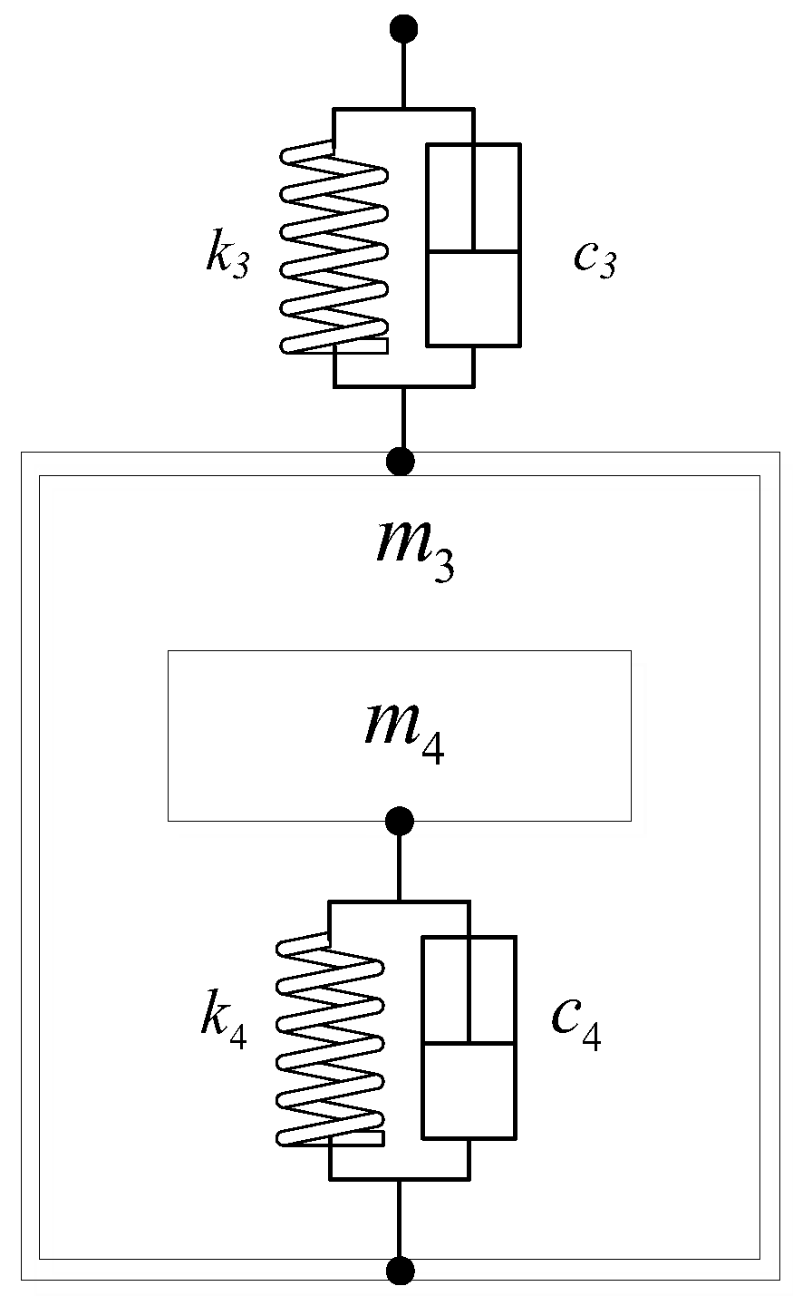
2. Elevator System Dynamics Modeling

This paper considers structural dynamics modeling methods, including centralized mass and distributed mass models, to study elevator system dynamics. Focusing solely on the longitudinal motion of each component, this paper employs the centralized mass model. Due to the numerous degrees of freedom in the dynamics model, this paper utilizes the finite element method to initially establish dynamics models for individual subsystems. These models are then centralized to derive the overall system’s dynamics model.

The high-speed elevator system is partitioned into eight subsystems: a car and frame subsystem, four sections of wire rope (a car side traction rope subsystem, a car side tensioning rope subsystem, a counterweight side traction rope subsystem, and a counterweight side tensioning rope subsystem), a traction subsystem, a counterweight subsystem, and a tensioning subsystem. These subsystems share degrees of freedom. The car and frame subsystem, traction subsystem, counterweight subsystem, and tensioning subsystem are linear, while the traction rope and tensioning rope are non-linear. For ease of subsequent model integration and numerical solution, the linear and non-linear subsystems are separately and independently managed. This ensures that during numerical computation, only the contribution of non-linear subsystems to the dynamics model is updated. Figure 1 depicts the process of establishing the dynamics model, encompassing degree of freedom selection, subsystem decomposition, subsystem dynamics modeling, and integration of the overall dynamics model. Within this, the subsystem dynamics modeling process comprises linear and non-linear subsystem dynamics modeling.

After integration, the overall dynamics equation of the elevator model can be expressed as follows:

$$\begin{array}{l}M\ddot{x}\left(\mathrm{t}\right)+C\dot{x}\left(\mathrm{t}\right)+Kx\left(\mathrm{t}\right)=F\\ M=M_{linear}+M_{no-linaer}\\ C=C_{linear}+C_{no-linaer}\\ K=K_{linear}+K_{no-linaer}\end{array}$$

(1)

where $M$ represents the equivalent mass matrix of the elevator system model, which can be expressed as:

$C,K$ is the equivalent damping matrix and the equivalent stiffness matrix of the elevator system model, similar to the structure $M$. Figure 2a depicts the overall dynamics model of the high-speed elevator, while Figure 2b illustrates the mechanical model of the high-speed elevator.

2.1. Non-Linear Subsystems

In traditional modeling, the elevator wire rope is typically considered as a fixed member with constant stiffness and damping arrays. However, in this paper, we treat the wire rope as a non-linear model. Both its stiffness and damping matrices are functions of time, and they are updated dynamically to reflect changes over time.

The elevator system has four sections of wire rope, each of which constitutes a non-linear subsystem, namely, the car side traction rope subsystem $\left(L_1\right)$, the counterweight traction rope subsystem $\left(L_2\right)$, the car side tensioning rope subsystem $\left(L_3\right)$, and the counterweight side tensioning rope subsystem $\left(L_4\right)$. As shown in Figure 3, each section of the rope is divided into a number of units, each of which corresponds to a small unit consisting of a mass, a spring, and damping.

The vertical displacement of nodes serves as the degrees of freedom in the discretized model of the wire rope, where neighboring units are connected by nodes. Generally, increasing the number of nodes enhances the accuracy of the dynamics model, albeit with a corresponding increase in computational workload.

In this paper, we take $n=5$. The wire rope in the elevator structure is divided into five small units in each of its four sections. The mass and stiffness of these units are non-linear and vary based on the elevator’s position during operation. The mass of the small unit of the four sections of wire rope can be expressed as:

$$\begin{array}{l}{m}_{L_{11}}=m_{L_{12}}=\dots =m_{L_{15}}=N_1{\rho }_1{l}_{t1}/5\\ m_{L_{21}}=m_{L_{22}}=\dots =m_{L_{25}}=N_1{\rho }_1(l_1-l_t)/5\\ m_{L_{31}}=m_{L_{32}}=\dots =m_{L_{35}}=N_2{\rho }_2{l}_{t2}/5\\ m_{L_{41}}=m_{L_{42}}=\dots =m_{L_{45}}=N_2{\rho }_2(l_2-l_{t2})/5\end{array}$$

(2)

where $m_{L_{11}},m_{L_{12}},m_{L_{13}},m_{L_{14}},m_{L_{15}}$ is the mass of the five small units of $L_1$, and the other three ropes are the same. $N_1,N_2$ is the number of traction wire ropes and tensioning wire ropes, ${\rho }_1,{\rho }_2$ is the wire density of the hauling and tensioning ropes, $l_1,l_2$ is the total length of the traction wire rope and tensioning wire rope, and $l_{t1},l_{t2}$ is the real-time length of the car side traction wire rope and car side tensioning wire rope. It can be expressed as:

$$\begin{array}{l}{l}_{t1}=h_1-h_2-h_t+h_3\\ l_{t2}=h_t+h_4\end{array}$$

(3)

where $h_1$ is the height of the shaft, $h_2$ is the height of the car frame, $h_3$ is the height of the top floor, $h_4$ is the height of the pit, and $h_t$ is the height of the car after the car starts running from the lowest floor and is a function of time $t$.

At this point, the total contributing mass matrix of the four wire rope subsystem models can be expressed as:

$$\left[M_L\right]=\left(\begin{array}{ccccc}{m}_{L_{11}}& & & & \\ & m_{L_{12}}& & & \\ & & \ddots & & \\ & & & m_{L_{44}}& \\ & & & & m_{L_{45}}\end{array}\right)$$

(4)

where $m_{L_{11}},m_{L_{12}},\cdots ,m_{L_{44}},m_{L_{45}}$ are all functions of time $t$, so $\left[M_L\right]$ will change with time. In this paper, we use matrix updating to express the time-varying nature of the mass matrix, and its expression is:

$$\begin{array}{c}\left[M_{L(t+1)}\right]=\left[M_{L(t)}\right]+\left[M_{L(t+1)}\right]\\ =\left(\begin{array}{ccccc}{m}_{L_{11}(t)}& & & & \\ & m_{L_{12}(t)}& & & \\ & & \ddots & & \\ & & & m_{L_{44}(t)}& \\ & & & & m_{L_{45}(t)}\end{array}\right)+\left(\begin{array}{ccccc}{m}_{L_{11}(t+1)}& & & & \\ & m_{L_{12}(t+1)}& & & \\ & & \ddots & & \\ & & & m_{L_{44}(t+1)}& \\ & & & & m_{L_{45}(t+1)}\end{array}\right)\end{array}$$

(5)

Similarly, the stiffness of the four sections of the wire rope is also affected by the length of the wire rope; the effective length of the wire rope changes and the stiffness also changes in real time, as expressed by the formula:

$$\begin{array}{l}{k}_{L_{11}}=k_{L_{12}}=\dots =k_{L_{15}}=E{A}_1/l_{t1}\\ k_{L_{21}}=k_{L_{22}}=\dots =k_{L_{25}}=E{A}_1/(l_1-l_{t1})\\ k_{L_{31}}=k_{L_{32}}=\dots =k_{L_{35}}=E{A}_2/l_{t2}\\ k_{L_{41}}=k_{L_{42}}=\dots =k_{L_{45}}=E{A}_2/(l_2-l_{t2})\end{array}$$

(6)

where $k_{L_{11}},k_{L_{12}},k_{L_{13}},k_{L_{14}},k_{L_{15}}$ is the stiffness of the five small units of $L_1$, and the other three ropes are the same. $E$ is the modulus of elasticity of the wire rope and $A_1,A_2$ is the cross-sectional area of the traction wire rope and tensioning wire rope.

The contributing stiffness matrices of the wire rope subsystem model can be expressed as:

$$\left[K_L\right]=\left(\begin{array}{ccccc}{k}_{L_{11}}& & & & \\ & k_{L_{12}}& & & \\ & & \ddots & & \\ & & & k_{L_{44}}& \\ & & & & k_{L_{45}}\end{array}\right)$$

(7)

Likewise, the stiffness matrix that contributes varies over time, and in this paper, we utilize an updating approach to illustrate its time-varying characteristics using the following expression:

$$\begin{array}{c}\left[K_{L(t+1)}\right]=\left[K_{L(t)}\right]+\left[K_{L(t+1)}\right]\\ =\left(\begin{array}{ccccc}{k}_{L_{11}(t)}& & & & \\ & k_{L_{12}(t)}& & & \\ & & \ddots & & \\ & & & k_{L_{44}(t)}& \\ & & & & k_{L_{45}(t)}\end{array}\right)+\left(\begin{array}{ccccc}{k}_{L_{11}(t+1)}& & & & \\ & k_{L_{12}(t+1)}& & & \\ & & \ddots & & \\ & & & k_{L_{44}(t+1)}& \\ & & & & k_{L_{45}(t+1)}\end{array}\right)\end{array}$$

(8)

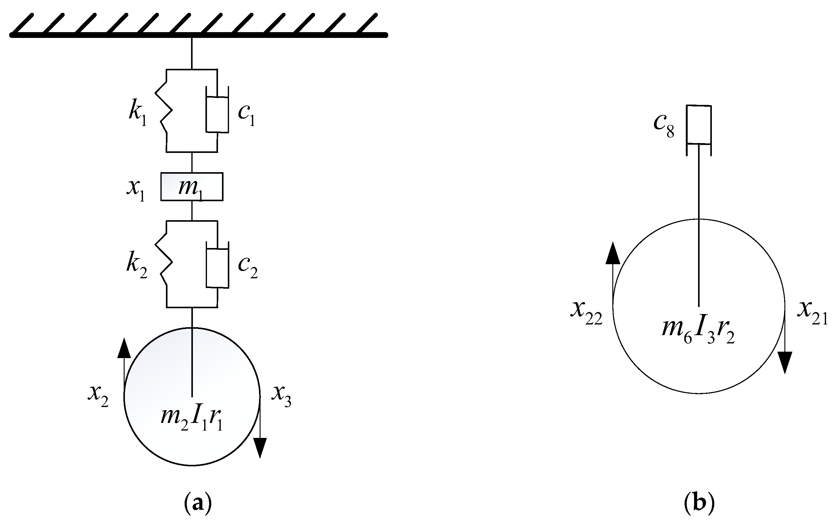
2.2. Linear Subsystem

Apart from the wire rope, all subsystems in the elevator system are linear. Newton’s law and Lagrange’s equation are applied to model the centralized mass of each subsystem.

The traction and tension subsystems in the elevator are complex, requiring the use of Lagrange equations to model their dynamics. Figure 4 illustrates the simplification of the elevator traction subsystem’s vibration isolation rubber to a spring damping system. Additionally, the mass of other components is concentrated to create a three-degree-of-freedom dynamics model for the traction subsystem.

In Figure 4, $x_1,x_2,x_3$ are the three degrees of freedom of the traction subsystem, $x_1$ is the centralized mass displacement of the tractor, $x_2$ is the displacement of the contact point of the traction sheave with the rope on the car side, and $x_3$ is the displacement of the contact point of the traction sheave with the rope on the counterweight side, and is specified in a generalized coordinate system, with the car moving upwards in the positive direction.

The kinetic energy of the traction subsystem can be expressed as:

$$T=\frac{1}{2}{m}_1{{\dot{x}}_1}^2+\frac{1}{2}{m}_2{\left(\frac{{\dot{x}}_2-{\dot{x}}_3}{2}\right)}^2+\frac{1}{2}{I}_1{\left(\frac{{\dot{x}}_2+{\dot{x}}_3}{2r_1}\right)}^2$$

(9)

The elastic potential energy of the traction subsystem can be expressed as:

$$V=\frac{1}{2}{k}_1{x}_1^2+\frac{1}{2}{k}_2{\left(\frac{x_2-x_3}{2}-x_1\right)}^2$$

(10)

The dissipated energy of the traction subsystem can be expressed as:

$$W=\frac{1}{2}{c}_1{\dot{x}}_1^2+\frac{1}{2}{c}_2{\left(\frac{{\dot{x}}_2-{\dot{x}}_3}{2}-{\dot{x}}_1\right)}^2$$

(11)

Substituting the above energy equation into the Lagrange equation:

$$\frac{d}{dx}\left(\frac{\partial T}{\partial \dot{x}}\right)-\frac{\partial T}{\partial x}+\frac{\partial V}{\partial x}+\frac{\partial W}{\partial \dot{x}}=F$$

(12)

Solving this yields the differential equation of motion for the traction subsystem:

$$M\ddot{x}+C\dot{x}+Kx=F$$

(13)

where the contributing mass matrix of the trailing subsystem is:

$$\left[M_1\right]=\frac{1}{4}\left(m_2+\frac{I_1}{r_1^2}\right)\left(\begin{array}{ccc}1& 0& 0\\ 0& 1& 0\\ 0& 0& 1\end{array}\right)+\frac{1}{4}\left(-m_2+\frac{I_1}{r_1^2}\right)\left(\begin{array}{ccc}0& 1& 0\\ 1& 0& 0\\ 0& 0& 0\end{array}\right)+m_1\left(\begin{array}{ccc}0& 0& 0\\ 0& 0& 0\\ 0& 0& 1\end{array}\right)$$

(14)

The contributing stiffness matrix is:

$$\left[K_1\right]=\frac{1}{4}{k}_2\left(\begin{array}{ccc}1& -1& -2\\ -1& 1& 2\\ -2& 2& 4\end{array}\right)+k_2\left(\begin{array}{ccc}0& 0& 0\\ 0& 0& 0\\ 0& 0& 1\end{array}\right)$$

(15)

The contribution damping matrix is:

$$\left[C_1\right]=\frac{1}{4}{c}_2\left(\begin{array}{ccc}1& -1& -2\\ -1& 1& 2\\ -2& 2& 4\end{array}\right)+c_1\left(\begin{array}{ccc}0& 0& 0\\ 0& 0& 0\\ 0& 0& 1\end{array}\right)$$

(16)

In the above formula, $m_1$ is the sum of the mass of the motor and the traction wheel support. $m_2$ is the equivalent mass of the traction wheel and the guide wheel. $k_1,k_2$ and $c_1,c_2$ are the stiffness and damping of the vibration isolation rubber on the upper and lower part of the traction wheel support, respectively. $I_1$ is the equivalent rotational moment of the traction wheel and $r_1$ is the radius of the traction wheel.

The tension subsystem functions similarly to the traction subsystem. It counterbalances the dynamic imbalance arising from elevator operation, connected with the compensation rope and located beneath the car and counterweight. Unlike the traction sheave, the tension sheave lacks vibration isolation rubber, with damping assumed to be 0. The same Lagrange equation can be used to obtain the contributing mass matrix $\left[M_2\right]$, the contributing stiffness matrix $\left[K_2\right]$, and the contributing damping matrix $\left[C_2\right]$ of the tension subsystem.

The car and frame subsystem and counterweight subsystem are simple linear substructure models with selected degrees of freedom. Newton’s second law is used to construct a dynamic model. $x_3,x_4,x_5$ are the three degrees of freedom of the car and frame subsystem, and the car and frame are connected to the traction wire rope on the side of the car through the node above the frame, and the displacement of this node is recorded as $x_3$. $x_4$ is the displacement of the car. The bottom node of the frame is directly connected to the tensioning wire rope, and the displacement of this node is recorded as $x_5$. This paper solely focuses on vertical vibrations, specifically addressing the vibration isolation rubber located at the bottom of the car, while disregarding the left and right vibration isolation rubber. The developed kinetic model is depicted in Figure 5.

In Figure 5, $m_3$ is the mass of the car frame, $m_4$ is the mass of the car, $k_3,c_3$ is the stiffness and damping of the rope head spring, and $k_4,c_4$ is the stiffness and damping of the vibration isolation rubber at the bottom of the car. According to Newton’s second law, to obtain the differential equation of the car and frame subsystem:

$$\begin{array}{l}{m}_3{\ddot{x}}_3+c_3\left({\dot{x}}_3-{\dot{x}}_4\right)+k_3\left(x_3-x_4\right)=0\\ m_4{\ddot{x}}_4+c_4\left({\dot{x}}_4-{\dot{x}}_5\right)+c_3\left({\dot{x}}_4-{\dot{x}}_3\right)+k_4\left(x_4-x_5\right)+k_3\left(x_4-x_3\right)=0\\ c_3\left({\dot{x}}_5-{\dot{x}}_4\right)+k_4\left(x_5-x_4\right)=0\end{array}$$

(17)

Solve the contributing mass matrix of the car and frame subsystem as:

$$\left[M_3\right]=\left(\begin{array}{ccc}{m}_3& & \\ & m_4& \\ & & 0\end{array}\right)$$

(18)

The contributing stiffness matrix is:

$$\left[K_3\right]=\left(\begin{array}{ccc}{k}_3& -k_3& 0\\ -k_3& k_3+k_4& -k_4\\ 0& -k_4& k_4\end{array}\right)$$

(19)

The contribution damping matrix is:

$$\left[C_3\right]=\left(\begin{array}{ccc}{c}_3& -c_3& 0\\ -c_3& c_3+c_4& -c_4\\ 0& -c_4& c_4\end{array}\right)$$

(20)

The counterweight subsystem mirrors the car and frame subsystem. It involves selecting the connection point of the rope head spring on the counterweight with the traction rope, along with the counterweight displacement, as degrees of freedom to construct the model. Newton’s second law is utilized to obtain the contributing mass matrix $\left[M_4\right]$, contributing stiffness matrix $\left[K_4\right]$, and contributing damping matrix $\left[C_4\right]$ of the counterweight subsystem.

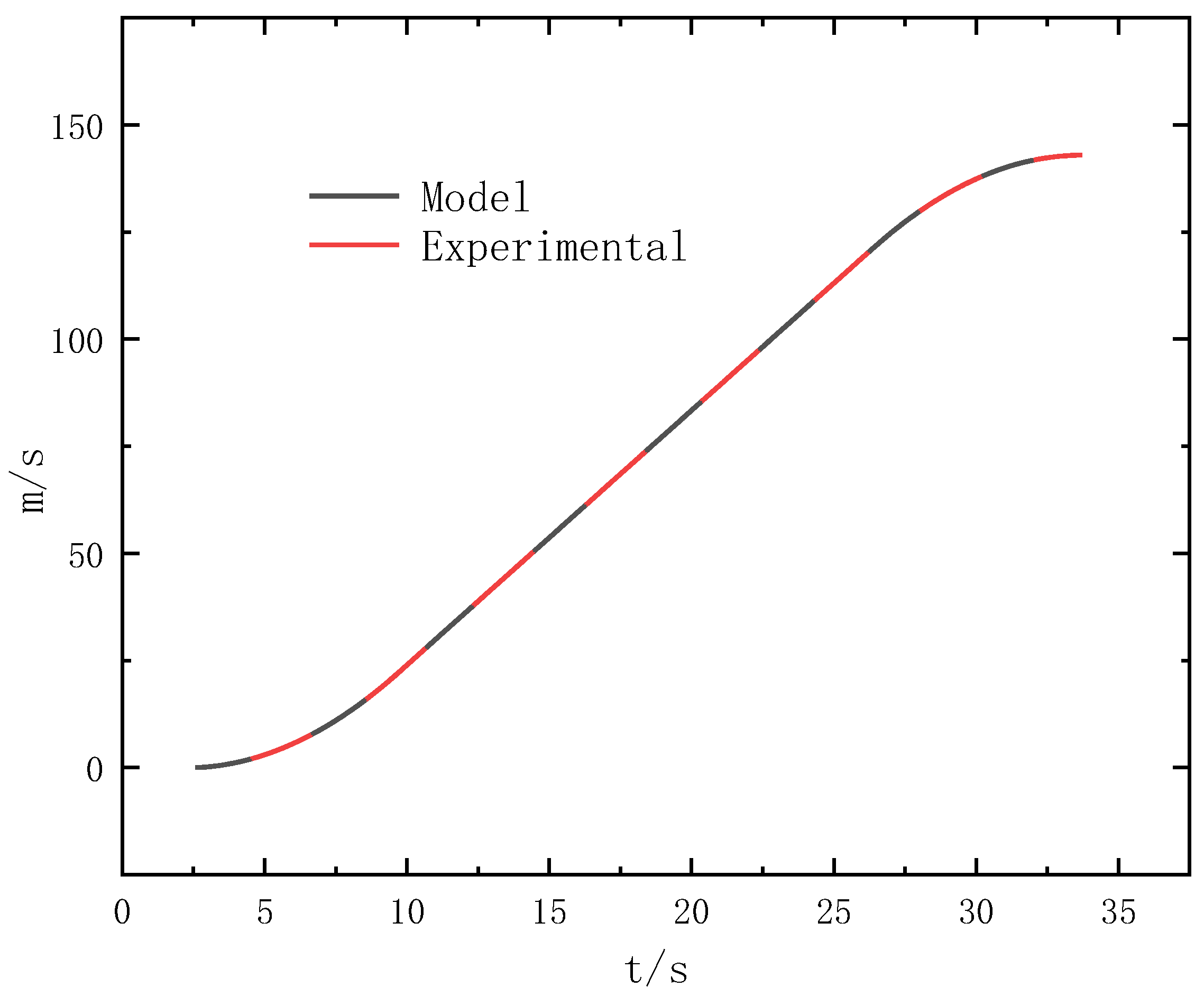
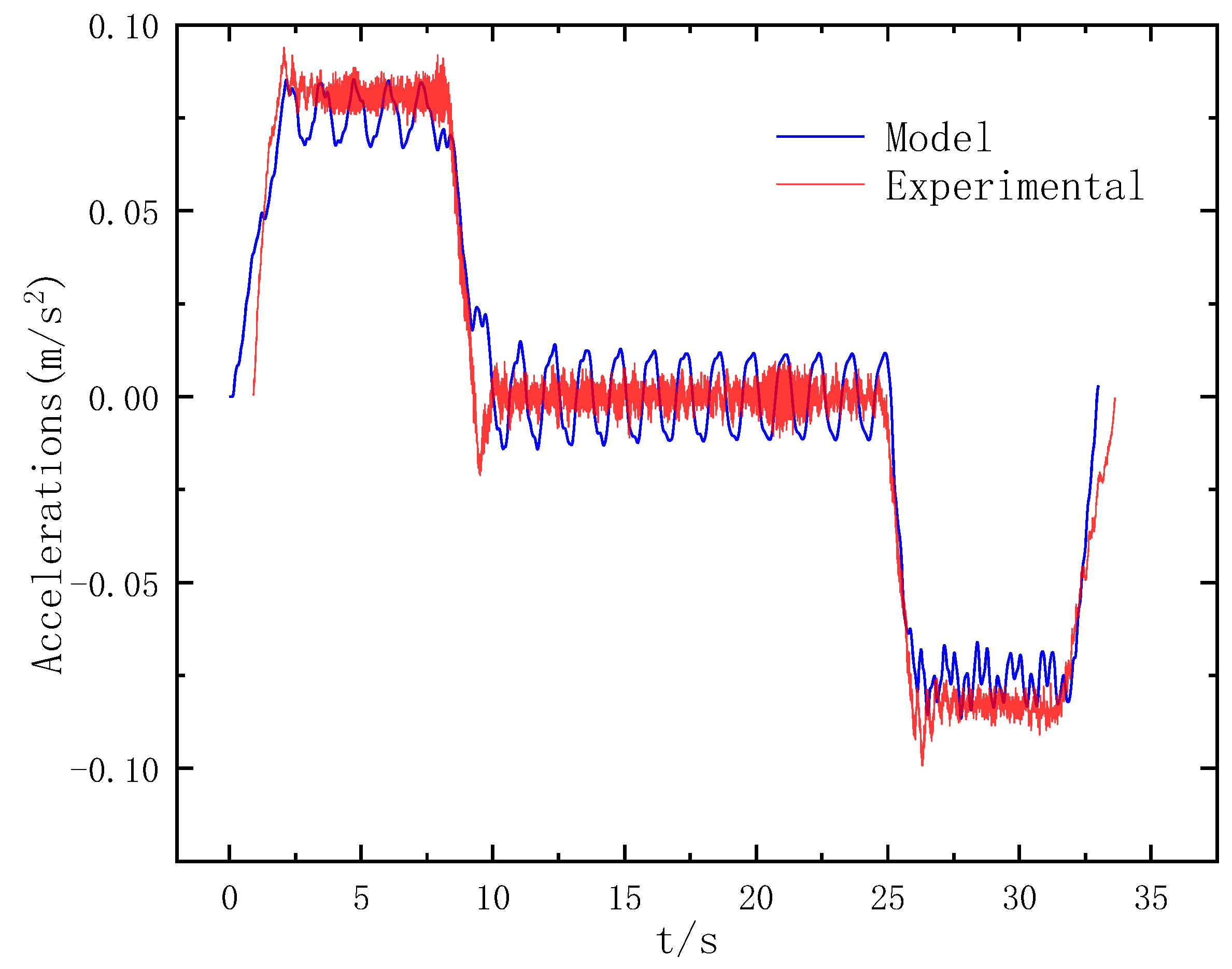
3. Time Domain Calculation Analysis

General elevator dynamics calculations often overlook the non-linear effects induced by the rigid dead rope components or linearize the non-linear aspects. Employing instantaneous structural assumptions, the entire system movement is segmented into n time intervals. In each interval, the dynamic system characteristics remain invariant, and the variable coefficient differential equations are transformed into constant coefficient ones for elevator calculation. Although this approach allows for an analysis of elevator dynamic characteristics, it neglects the influence of vibrations on the overall elevator motion, as well as the impact of non-linear components such as the wire rope. This study utilizes the fourth-order Runge–Kutta method with a variable step size for time-domain step-by-step integration of the elevator systems’ differential equations with variable coefficients. Utilizing a Fortran algorithm, numerical calculations are conducted. Considering the elevator’s overall operational pattern and corresponding vibration effects, time-domain step-by-step integration offers a superior stability compared to division into multiple time intervals, concurrently enhancing the computational accuracy.

The system $x$ is the displacement of each degree of freedom, $\dot{x}$ is the velocity of each degree of freedom, and $\ddot{x}$ is the acceleration of each degree of freedom. The elevator dynamics equation is:

$$M\ddot{x}\left(\mathrm{t}\right)+C\dot{x}\left(\mathrm{t}\right)+Kx\left(\mathrm{t}\right)=F$$

(21)

where $M$ is the equivalent mass matrix of the elevator system model, $C$ is the equivalent damping matrix of the elevator system model, $K$ is the equivalent stiffness matrix of the elevator system model, and $F$ is the external excitation of the elevator system related to the control strategy. The generalized acceleration vector of the elevator system can be expressed as follows:

$$\ddot{x}\left(t\right)=M^{-1}\left(F-C\dot{x}\left(t\right)-Kx\left(t\right)\right)$$

(22)

Considering the elevator degree-of-freedom displacement $x$ and the elevator degree-of-freedom velocity $\dot{x}$ as unknown, define a new vector $X\left(\mathrm{t}\right)=\left[\begin{array}{c}x\left(t\right)\\ \dot{x}\left(t\right)\end{array}\right]$. Then,

$$\dot{X}\left(t\right)=\left[\begin{array}{c}\dot{x}\left(t\right)\\ \ddot{x}\left(t\right)\end{array}\right]=\left[\begin{array}{c}\dot{x}\\ M^{-1}\left(F-C\dot{x}-Kx\right)\end{array}\right]$$

(23)

Then,

$$\dot{X}\left(t\right)=\left[\begin{array}{cc}0& I\\ -M^{-1}K& -M^{-1}C\end{array}\right]\left[\begin{array}{c}x\left(t\right)\\ \dot{x}\left(t\right)\end{array}\right]+\left[\begin{array}{c}0\\ M^{-1}F\end{array}\right]=AX\left(t\right)+F\left(t\right)$$

(24)

where

$$A=\left[\begin{array}{cc}0& I\\ -M^{-1}K& -M^{-1}C\end{array}\right],F\left(t\right)=\left[\begin{array}{c}0\\ M^{-1}F\end{array}\right]$$

(25)

Based on the variable-step-length fourth-order Runge–Kutta method, this can be derived as:

$$X_{i+1}=X_i+\frac{1}{6}\left(K_1+2K_2+2K_3+K_4\right)$$

(26)

Included among these are:

$$\begin{array}{l}{K}_1=f\left(X_i,t_i\right)\\ K_2=f\left(X_i+\frac{h}{2}{K}_1,t_i+\frac{h}{2}\right)\\ K_3=f\left(X_i+\frac{h}{2}{K}_2,t_i+\frac{h}{2}\right)\\ K_4=f\left(X_i+2h{K}_3,t_{i+1}+h\right)\end{array}$$

(27)

The computational flow is shown in Figure 6:

The elevator control strategy was established with a calculation step of 0.001 s, inputting the elevator’s basic parameters and utilizing the dynamics model and numerical algorithm provided in this paper to compute the elevator’s displacement and acceleration. The computed values were compared with experimental data obtained from a company. The basic parameters of the high-speed elevator are detailed in

Table 1. Basic parameters of the high-speed elevator.

Elevator Parameter	Unit	Numeric
Racking girder quality	kg	198.45
Equivalent mass of traction device	kg	2835
Carriage quality	kg	2282
Car mass	kg	1805
Counterweight mass	kg	4887.4
Compensation system quality	kg	1260
Moment of inertia of the traction sheave	kg·m2	50
Compensating wheel moment of inertia	kg·m2	51.5
Stiffness of the upper vibration isolation rubber of the traction unit	N/m	1.6 $\times$ 107 $\times$ 4
Stiffness of vibration isolation rubber underneath the traction unit	N/m	2.7 $\times$ 107 $\times$ 4
Car side rope head taper sleeve spring stiffness	N/m	2.72 $\times$ 105 $\times$ 15
Anti-vibration rubber stiffness of car bottom	N/m	9.8 $\times$ 105 $\times 6$
Counterweight side rope head taper sleeve spring stiffness	N/m	2.72 $\times$105$\times$15
Number of ropes	roots	15
Traction rope line density	kg/m	0.494
Cross-sectional area of the rope	m2	1.2$\times$10−5
Young’s modulus of traction rope	N/m−2	1.176$\times$1011
Number of compensating ropes	roots	7
Compensating rope density	kg/m	0.878
Young’s modulus of compensating rope	N/m−2	9.8$\times$1010
Compensating rope cross-sectional area	m2	1.6$\times$10−5

, and the outcomes are depicted in Figure 7 and Figure 8.

In this study, an elevator-specific vibration analyzer was employed to gather vibration signals from the experimental tower of a company’s elevator. Data were collected using a three-axis acceleration sensor, transmitted to the terminal for processing, and output to obtain the experimental results.

Figure 7 demonstrates that the calculated results closely align with the displacement of the experimental test results. Additionally, Figure 8 reveals that the calculated acceleration closely matches the test results, despite the latter containing more complex excitations due to the diverse excitation force encountered during elevator operation. These outcomes underscore the accuracy of the dynamics model and numerical calculation method proposed in this paper, rendering them suitable for investigating the elevator’s dynamic properties.

4. Study of the Nature and Law of Elevator Dynamics

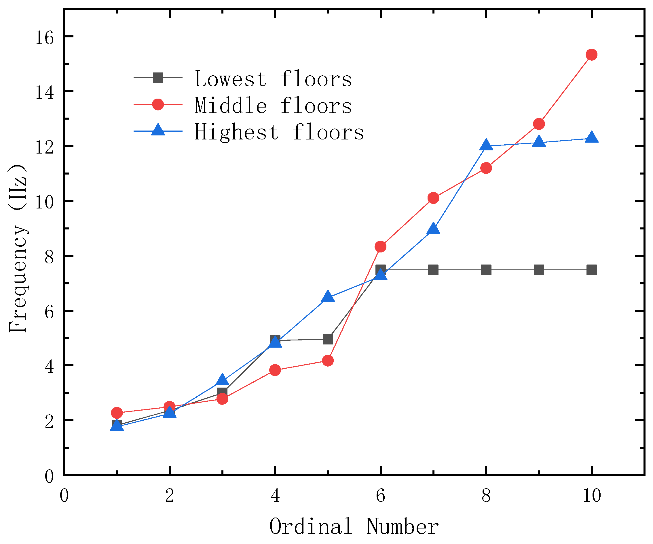
4.1. Effect of Car Height Position on Intrinsic Frequency

The mass and stiffness of both the car and counterweight side’s traction rope and compensation rope change with the elevator’s height, necessitating an analysis of the car’s intrinsic frequency at different positions. Using computations, we determined the intrinsic frequency at varying heights, illustrated in Figure 9. This includes elevators running at 10 m (lowest level), 80 m (middle level), and 140 m (highest level).

Figure 9 shows significant variations in the intrinsic frequency due to changes in the car’s height, primarily influenced by the non-linear mechanical properties of the wire rope. Notably, when the car is positioned in the middle, the first-order intrinsic frequency reaches its peak, attributed to the normal length of both the traction wire rope and the static tensioning wire rope. As the car ascends, the traction wire rope’s length decreases, consequently reducing the elevator’s fundamental frequency.

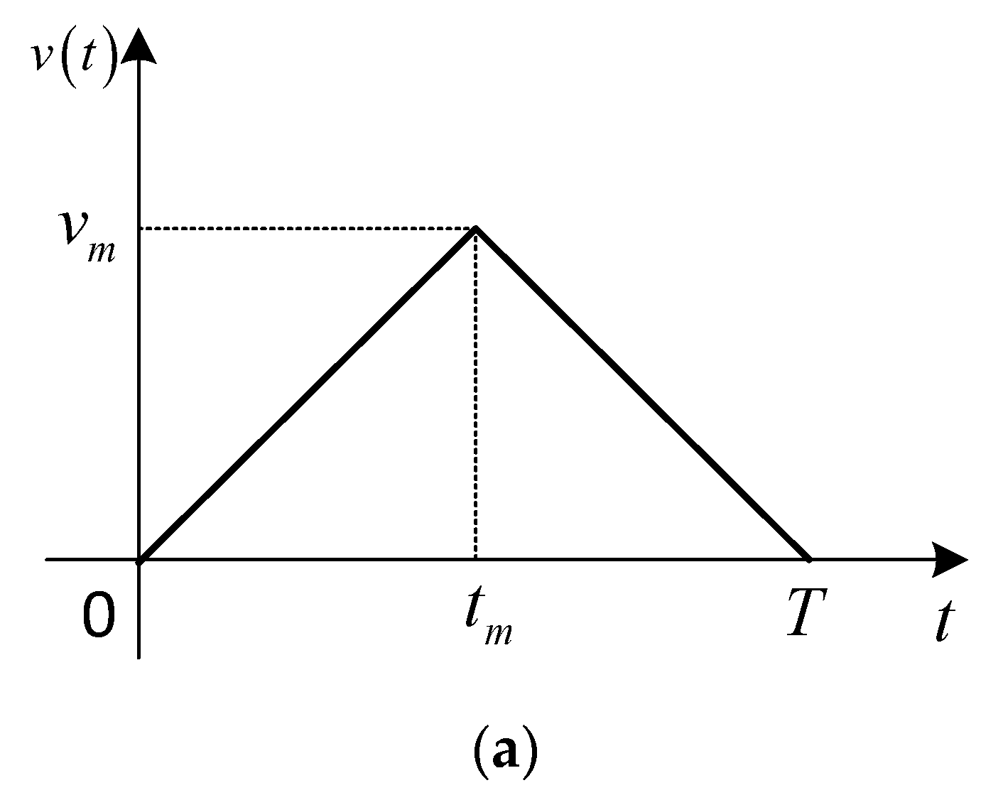
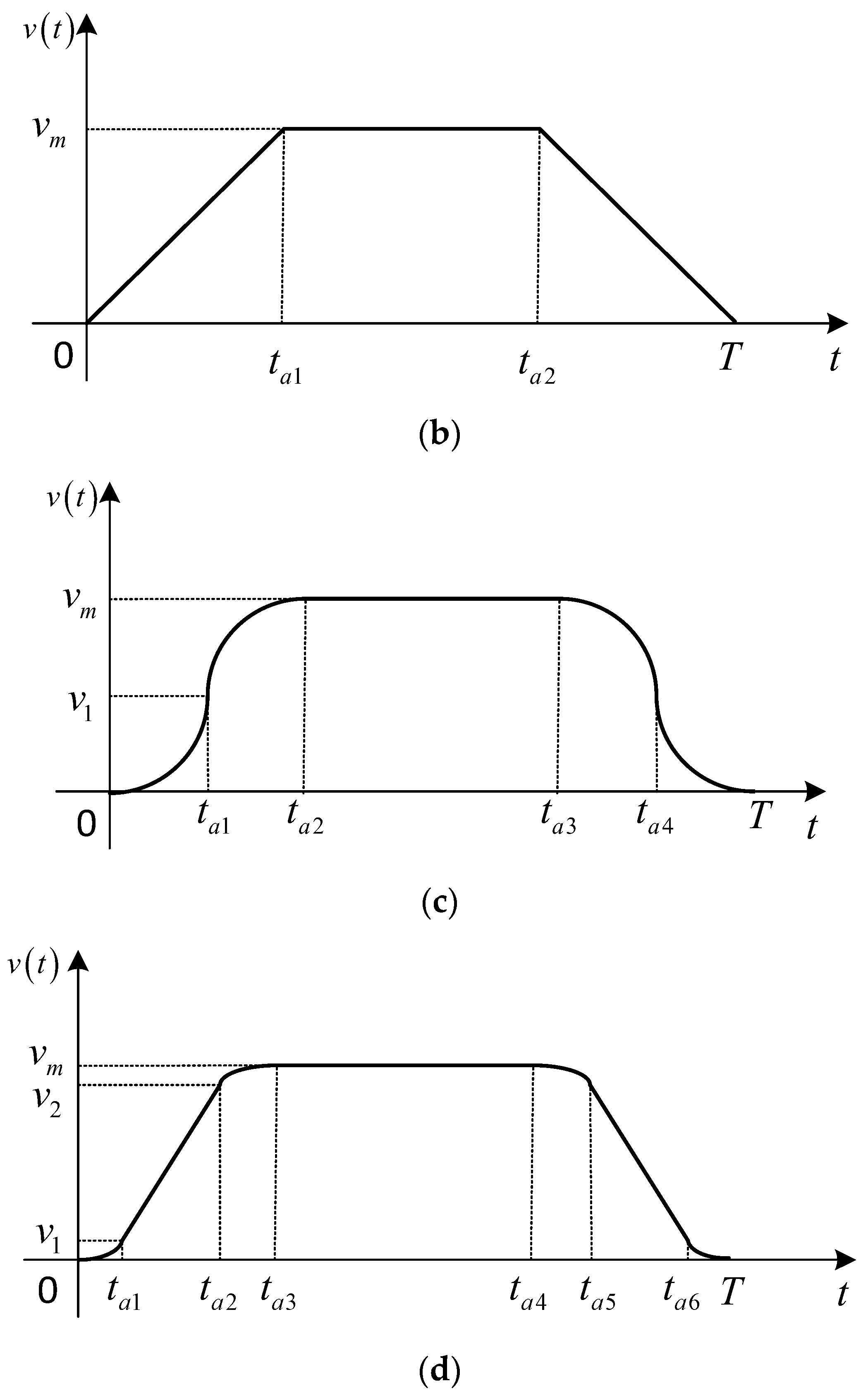
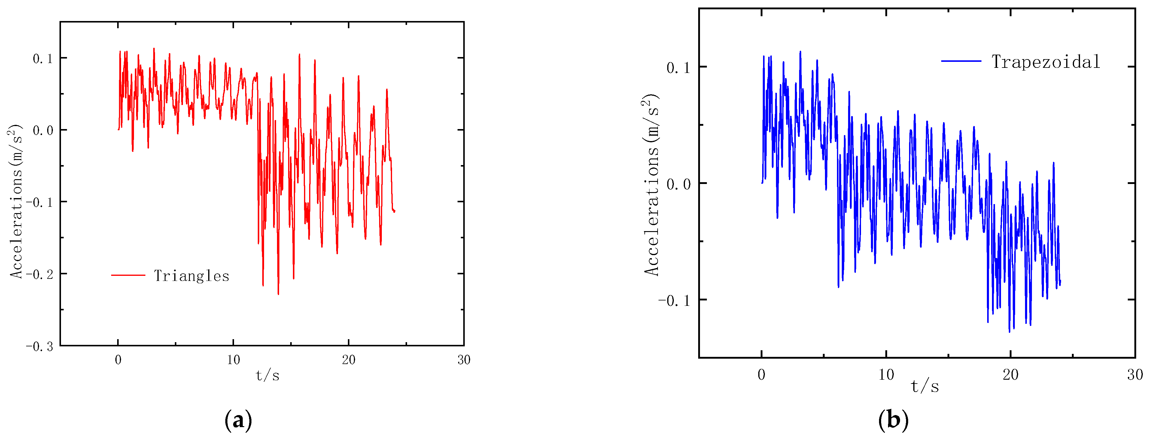
4.2. Impact of Control Strategies on Elevator Operation

During high-speed elevator operation, frequent acceleration and deceleration occur, significantly impacting passengers’ ride experience. Experimental findings indicate that passengers’ sensation of sinking and floating in the elevator correlates directly with the acceleration and rate of acceleration change. Excessive acceleration can lead to significant discomfort for passengers. Moreover, recognizing the impact of frequent acceleration and deceleration on elevator operation efficiency and costs, studying the elevator’s ideal speed curve, and selecting suitable motion laws are essential for enhancing the operation quality.

Currently, four common operating profiles are utilized for high-speed elevators: triangle, trapezoid, parabolic, and parabolic-linear composite shapes. Figure 10 illustrates the speed curves corresponding to these control strategies.

The basic parameters of the aforementioned high-speed elevator were input and the elevator control strategies were sequentially defined. Using a time step of 0.001 s, calculations were conducted to derive the acceleration response maps for the four conventional operational laws. The outcomes are illustrated in Figure 11.

Figure 11a illustrates the response of the triangular control strategy, showing significant fluctuations throughout the process. In Figure 11b, the response obtained from the trapezoidal control strategy demonstrates three distinct phases corresponding to acceleration, constant speed, and deceleration. Notably, fluctuations are prominent across these phases, particularly evident during the constant speed interval. The triangular and trapezoidal control strategies exhibit abrupt speed changes at the beginning and end of acceleration and deceleration, leading to discomfort for passengers due to sudden transitions in speed during the intermediate phases from acceleration to constant speed and constant speed to deceleration. Hence, they are unsuitable as operation laws for high-speed elevators.

Figure 11c,d depict the response diagrams of the line control strategy and the parabolic–linear control strategy, respectively. The response of both control strategies is roughly divided into three segments, corresponding to acceleration, constant speed, and deceleration. Notably, during the acceleration phase, the response of the parabolic–linear control strategy exhibits greater and more prolonged fluctuations compared to the parabolic control strategy due to an additional segment of uniform acceleration. This additional stage allows the elevator to reach a given speed faster. Conversely, in the constant speed phase, the response of the parabolic–linear control strategy demonstrates smaller fluctuations compared to the parabolic strategy. Similar to the acceleration phase, in the deceleration phase, the parabolic–linear control strategy’s response is better suited for high-speed elevators.

4.3. Effect of Load on Elevator Response

To investigate the impact of load on the time-domain response of the high-speed elevator, we selected the parabolic–linear control strategy. We then modified the load conditions of the car in the model to represent empty, half-loaded (800 kg), and fully loaded (1600 kg) scenarios. Subsequently, we calculated and compared the elevator’s time-domain response for each case. The results are presented in Figure 12.

As shown in Figure 12, during acceleration, the load minimally influences the time-domain response of the high-speed elevator. The responses of the three conditions are relatively similar at this stage. However, as the speed reaches the evaluated speed, the impact of the load on the elevator’s time-domain response becomes more pronounced. The elevator with a full load exhibits the highest fluctuation with the lowest frequency, while the empty elevator has the lowest fluctuation with the highest frequency. This effect persists until the deceleration phase. During the deceleration phase, the response fluctuations of the half-load and full-load conditions are similar to each other, but both are larger compared to the no-load condition.

4.4. Effect of Car Position Height on Elevator Response

The operational height impacts both the traction rope and compensation rope, two non-linear components of the elevator, consequently influencing the time-domain response. Similarly, to investigate the influence of the operational height on the time-domain response of a high-speed elevator, the control strategy was chosen as the parabolic–linear control approach. Given the minimal effect of no load on the time-domain response, the elevator was assumed to have no load. The operational height of the elevator was then segmented into the lowest (10 m), middle (80 m), and highest floors (140 m), and the model was computed accordingly. The comparative results are illustrated in Figure 13.

It can be observed from Figure 13 that the magnitude of time-domain response fluctuations is significantly higher at the highest level during the acceleration, uniform speed, and deceleration sections, compared to the lower and middle levels. During the acceleration phase, the response fluctuations at the lowest and middle levels are similar in magnitude, corresponding to the frequency of the car, which is close to the middle level. However, in the uniform speed section, the response fluctuations at the middle level are smaller than those at the lowest level, attributable to the elevator’s ascent to the middle floor. At this point, the distribution of the traction rope and compensation rope is more uniform, resulting in a higher intrinsic frequency. Conversely, during the deceleration phase, when the car is at the middle and lowest floors, the response magnitudes and frequencies are similar. This is because at the lowest floor, the traction rope is longest and the tensioning rope is shortest, while at the highest floor, the reverse is true.

5. Conclusions

This paper employs a combined approach of dynamic theoretical modeling and experimental control to develop a high-speed elevator model. The accuracy of this model is verified, serving as the foundation for investigating the longitudinal time-domain response of a high-speed elevator. The following conclusions are drawn from this study:

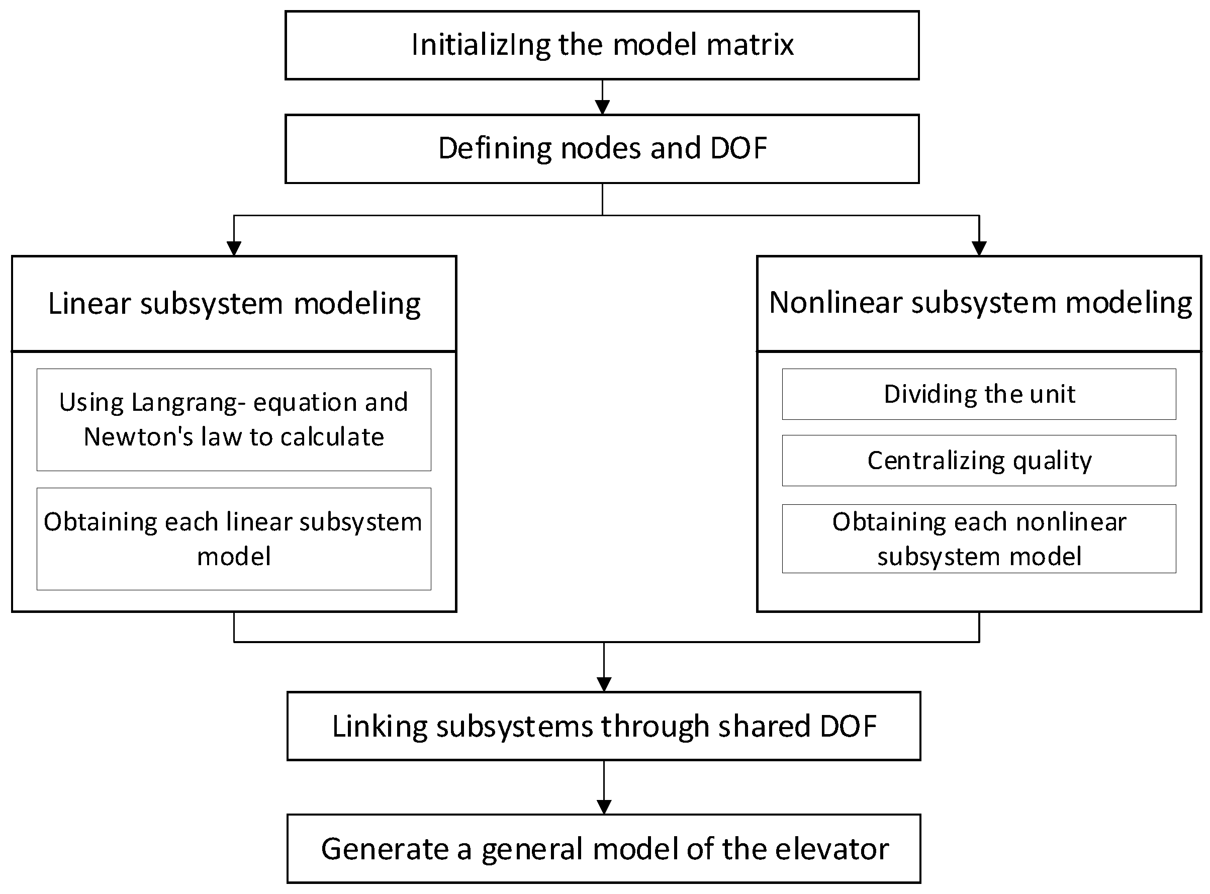
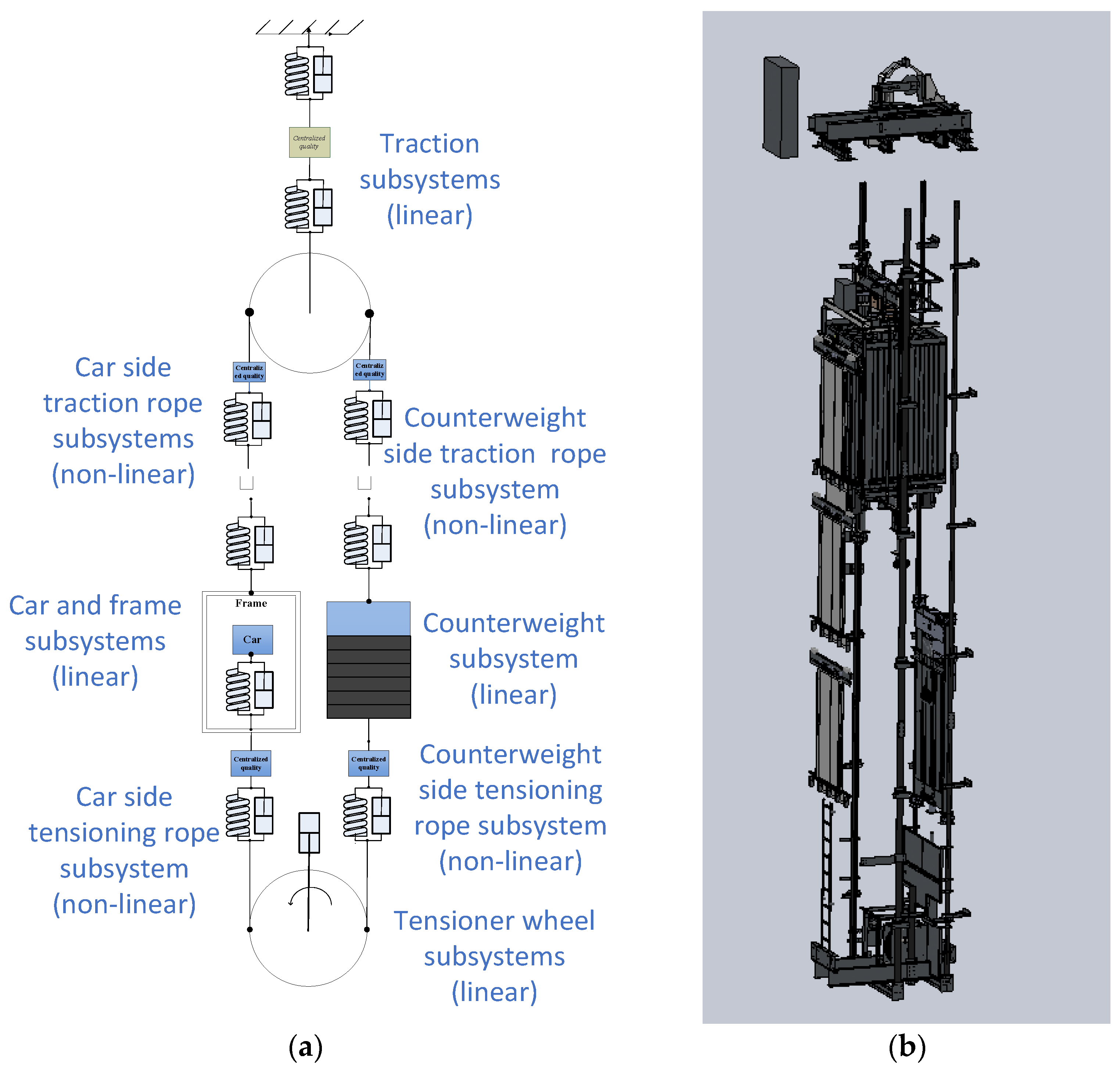
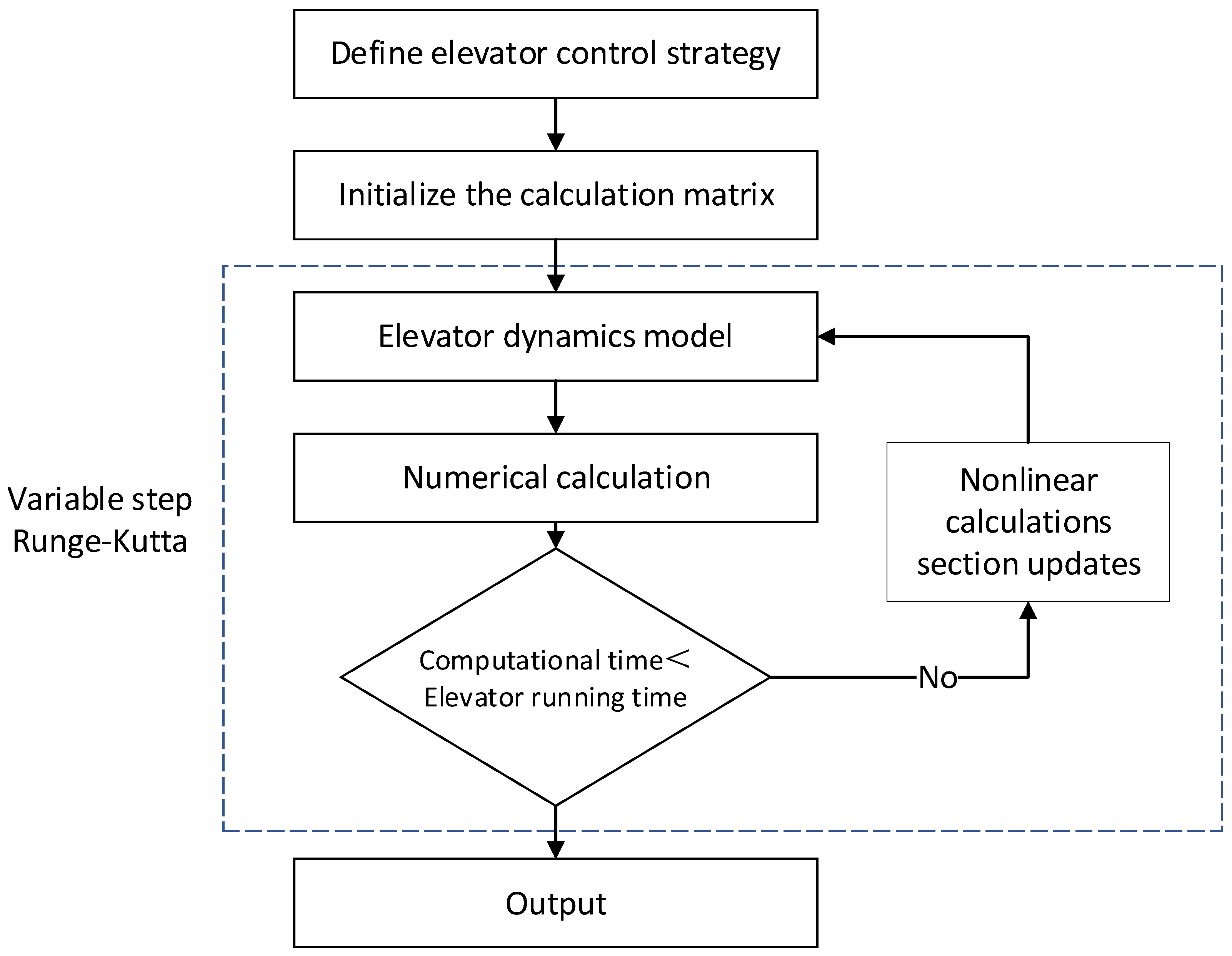
• This paper introduces a novel approach to analyze elevator system dynamics by dividing it into eight subsystems, developing a dynamics model for each and then integrating them based on shared degrees of freedom, providing an efficient and adaptable methodology. The time-domain calculation of the model employs stepwise integration, utilizing the variable-step fourth-order Runge–Kutta method. Comparison of the calculation results with experimental data confirms the feasibility of the model for time-domain analysis.
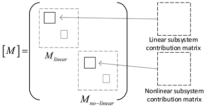
• This paper introduces a novel computational approach for handling the non-linear aspects of elevator dynamics. The linear and non-linear systems are separated during modeling, updating only the non-linear part in the numerical solution. This method circumvents the need for re-establishing the dynamics model, streamlining the computational process.
• With varying car heights, the length of each wire rope section fluctuates, consequently significantly altering the natural frequency of the elevator system. Specifically, when the car is positioned centrally, the first-order natural frequency of the elevator increases, leading to a reduction in its vibration response.
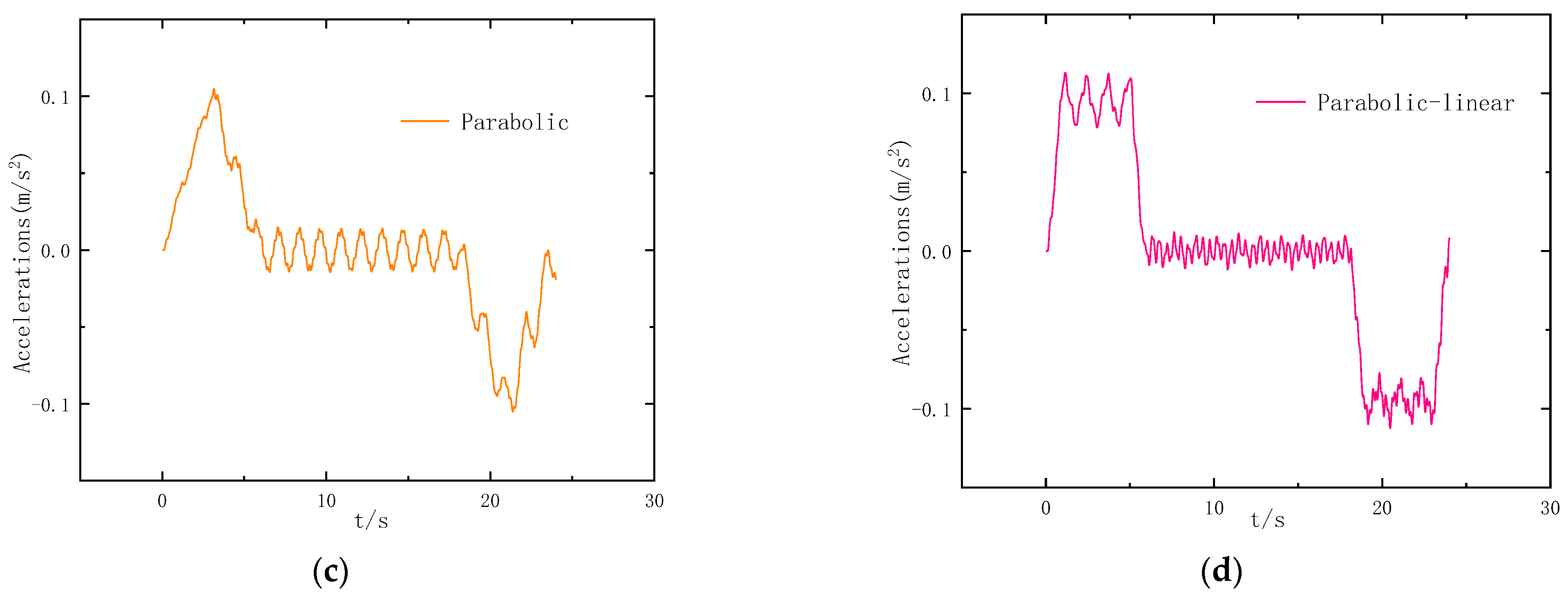
• Among the four common elevator control strategies, the triangle and trapezoidal control strategies result in significant elevator vibration response due to their abrupt initial and braking acceleration, rendering them unsuitable for high-speed elevators. Conversely, the parabolic and parabolic–linear control strategies exhibit minimal vibration responses, accompanied by gentle acceleration and deceleration. Hence, the parabolic–linear control strategy emerges as the preferable operational law for high-speed elevators.
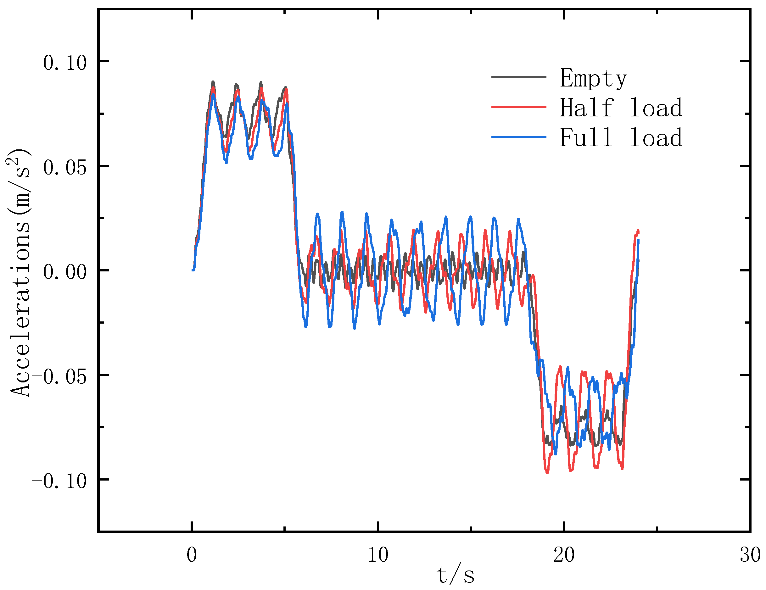
• The load variation significantly impacts the elevator’s time-domain response, notably evident during the uniform speed phase. The elevator’s vibration response increases and the natural frequency diminishes with an increasing load during operation at a uniform speed. Conversely, the vibration response remains similar across different loads during the acceleration phase. In the deceleration phase, no load results in the lowest response fluctuations, while a half load exhibits the most significant fluctuations.
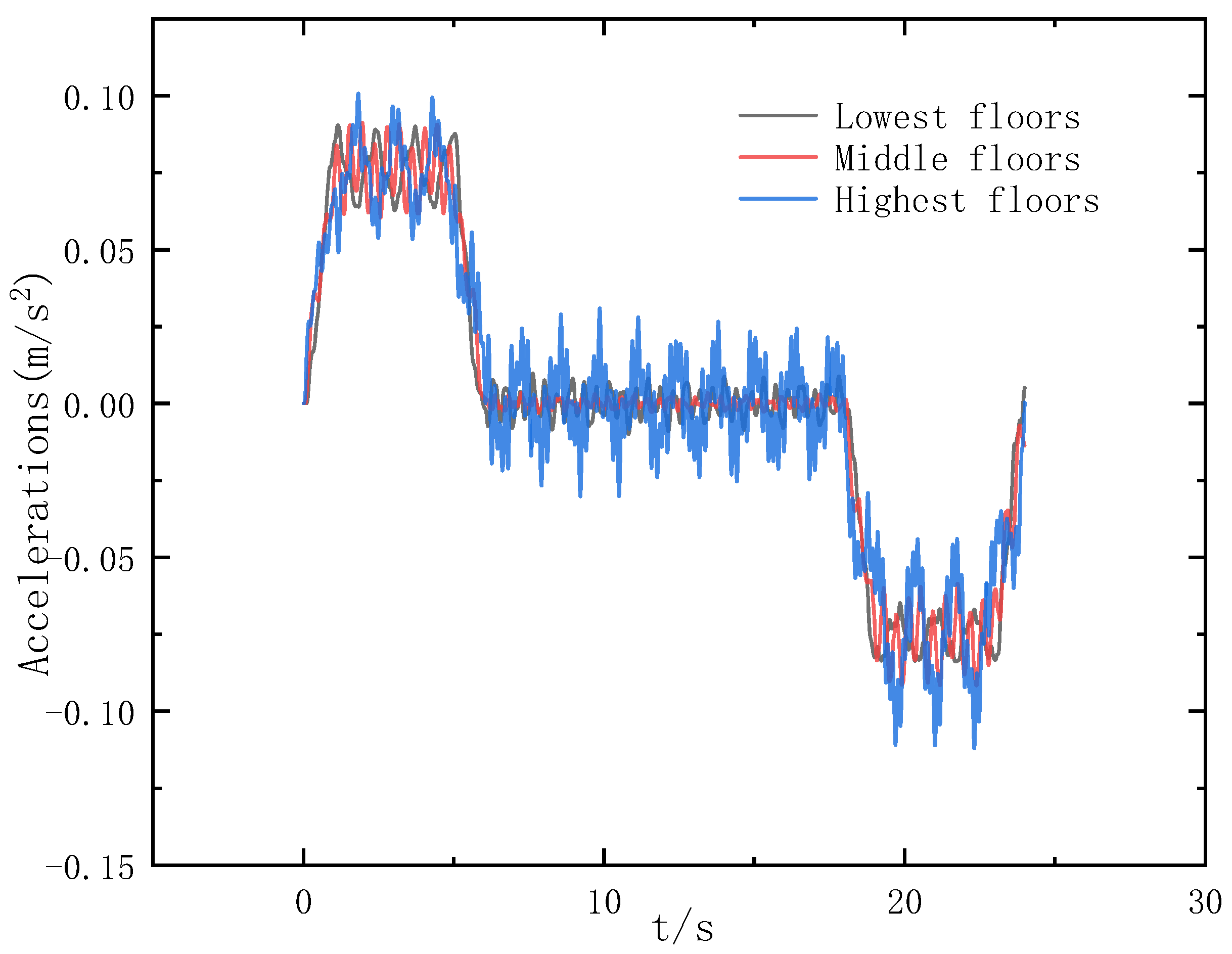
• The elevator’s vibration response is influenced by the changing mechanical properties of the wire rope at different car heights. During acceleration, the highest-level car exhibits the largest vibration response, while those at middle and lowest levels are similar. In the uniform speed phase, the highest-level car experiences larger vibration responses compared to those at the middle and lowest levels, with the middle-level car exhibiting the smallest response. Similarly, during deceleration, the highest-level car displays a greater vibration response than the middle- and lowest-level cars.

In conclusion, this paper establishes a theoretical foundation for computing the time-domain response of high-speed elevators and offers an efficient research approach for investigating the parameters that influence the responses in other high-speed elevators. Given the complexity of high-speed elevators, involving numerous parts and parameters, further studies on parameter optimization are warranted. Achieving the optimal elevator configuration and effective vibration damping necessitates continued research utilizing the model presented herein.

References

1. Zhang, Q.; Yang, Z.; Wang, C.; Yang, Y.; Zhang, R. Intelligent control of active shock absorber for high-speed elevator car. Proc. Inst. Mech. Eng. Part C J. Mech. Eng. Sci. 2019, 233, 3804–3815. [Google Scholar] [CrossRef]
2. Roberts, R. Control of high-rise/high-speed elevators. In Proceedings of the American Control Conference, Philadelphia, PA, USA, 26 June 1998; pp. 3440–3444. [Google Scholar]
3. Yu, Y. Research on Vibration Characteristics of High-Speed Traction Elevator Mechanical System. Master’s Thesis, Shandong University of Architecture, Jinan, China, 2015. [Google Scholar]
4. Peng, Q.; Jiang, A.; Yuan, H.; Huang, G.; He, S.; Li, S. Study on Theoretical Model and Test Method of Vertical Vibration of Elevator Traction System. Math. Probl. Eng. 2020, 2020, 8518024. [Google Scholar] [CrossRef]
5. Peng, Q.F.; Xu, P.; Yuan, H.; Ma, H.X.; Xue, J.H.; He, Z.Y.; Li, S.Q. Analysis of Vibration Monitoring Data of Flexible Suspension Lifting Structure Based on Time-Varying Theory. Sensors 2020, 20, 6586. [Google Scholar] [CrossRef] [PubMed]
6. Li, D.; Sun, G. Study on vertical time-varying vibration characteristics of traction-driven elevator. Mech. Eng. Autom. 2022, 1–12. [Google Scholar]
7. Xu, P.; Peng, Q.F.; Jin, F.S.; Xia, F.; Xue, J.H.; Yuan, H.; Li, S.Q. Experimental study on damping characteristics of elevator traction system. Adv. Mech. Eng. 2022, 14, 168781322210854. [Google Scholar] [CrossRef]
8. Dokic, R.; Vladic, J.; Kljajin, M.; Jovailovic, V.; Markovic, G.; Karakasic, M. Dynamic Modelling, Experimental Identification and Computer Simulations of Non-Stationary Vibration in High-Speed Elevators. Stroj. Vestn. J. Mech. Eng. 2021, 67, 287–301. [Google Scholar]
9. Shi, R.D.; Zhang, Q.; Zhang, R.J.; He, Q.; Liu, L.X. Analysis of the horizontal vibration response under gas-solid coupling throughout the entire high-speed elevator operating process. J. Vib. Control 2023, 29, 4455–4465. [Google Scholar] [CrossRef]
10. Du, X.Q.; Mei, D.Q.; Chen, Z.C. Research on the vertical dynamics of high-speed elevator system—Art. no. 60400V. In Proceedings of the 3rd International Conference on Mechatronics and Information Technology (ICMIT 05), Chongqing, China, 20–23 September 2005; p. V400. [Google Scholar]
11. Song, D.L.; Zhang, P.; Wang, Y.H.; Du, C.H.; Lu, X.M.; Liu, K. Horizontal dynamic modeling and vibration characteristic analysis for nonlinear coupling systems of high-speed elevators and guide rails. J. Mech. Sci. Technol. 2023, 37, 643–653. [Google Scholar] [CrossRef]
12. Zubik-Kowal, B. Dynamic Iterations for Nonlinear Systems Applied in Population Dynamics. In Proceedings of the 21st European Conference on Mathematics for Industry, ECMI, Wuppertal, Germany, 13–15 April 2021; pp. 91–97. [Google Scholar]
13. Qiu, L.M.; He, C.; Yi, G.D.; Zhang, S.Y.; Wang, Y.; Rao, Y.; Zhang, L.C. Energy-Based Vibration Modeling and Solution of High-Speed Elevators Considering the Multi-Direction Coupling Property. Energies 2020, 13, 4812. [Google Scholar] [CrossRef]
14. Tusset, A.M.; Fuziki, M.E.K.; Lenzi, G.G.; Santos, G.P.D.; Balthazar, J.M.; Brasil, R. Non-linear Energy Sink Applied in the Vibration Suppression of a High-Speed Elevator System and Energy Harvesting. J. Vib. Eng. Technol. 2023, 11, 2819–2830. [Google Scholar] [CrossRef]
15. Liu, S.C.; Wu, J.D.; Li, S.; He, D.Y.; Ji, Y.L. Multi-degree-of-freedom dynamic response calculation and experimental validation of a new type of vibrating relaxation screen. Vib. Shock 2023, 42, 48–54. [Google Scholar]
16. Qiu, C.J.; Zhang, L.X.; Li, M.H.; Zhang, P.P.; Zheng, X. Elevator Fault Diagnosis Method Based on IAO-XGBoost under Unbalanced Samples. Appl. Sci. 2023, 13, 10968. [Google Scholar] [CrossRef]
17. Wang, N.G.; Cao, G.H.; Wang, L.; Lu, Y.; Zhu, Z.C. Modelling and control of flexible guided lifting system with output constraints and unknown input hysteresis. J. Vib. Control 2020, 26, 112–128. [Google Scholar] [CrossRef]
18. Han, J. Intrinsic Characterization and Dynamic Response of Mechanical Vibration System of Traction Elevator. South Agric. Mach. 2021, 52, 3. [Google Scholar]
19. Fu, W.J.; Zhu, C.M.; Zhang, C.Y. Dynamic modeling and simulation analysis of a single winding elevator. J. Syst. Simul. 2005, 17, 635–638. [Google Scholar]
20. Lonkwic, P. Influence of friction drive lift gears construction on the length of braking distance. Chin. J. Mech. Eng. 2015, 28, 363–368. [Google Scholar] [CrossRef]
21. Peng, Q.F.; Xu, P.; Li, Y.K.; Yuan, H.; Xue, Z.N.; Yang, J.C. Experiment Research on Emergency Stop Vibrations of Key Components in the Friction Vertical Lifting System. Shock Vib. 2022, 2022, 7816270. [Google Scholar] [CrossRef]
Figure 1. Flowchart of the dynamics model.
Applsci 14 01821 g001
Figure 2. High-speed elevator model. (a) Overall model of high-speed elevator dynamics; (b) high-speed elevator mechanical model.
Applsci 14 01821 g002
Figure 3. Discrete model of a wire rope.
Applsci 14 01821 g003
Figure 4. Structure of traction and tensioning sheaves. (a) Traction subsystem; (b) tension subsystem.
Applsci 14 01821 g004
Figure 5. Car and frame subsystem.
Applsci 14 01821 g005
Figure 6. Flowchart of time domain computation.
Applsci 14 01821 g006
Figure 7. Comparison of experimental and modeled displacements.
Applsci 14 01821 g007
Figure 8. Comparison of experimental and modeled acceleration.
Applsci 14 01821 g008
Figure 9. Comparison of elevator frequencies at different operating heights.
Applsci 14 01821 g009
Figure 10. Speed profiles of four control strategies. (a) Triangular control strategy speed profile; (b) trapezoidal control strategy speed profile; (c) parabolic control strategy velocity profile; (d) parabolic–linear control strategy velocity profile.
Applsci 14 01821 g010aApplsci 14 01821 g010b
Figure 11. Time domain response under four different control strategies. (a) Triangular control strategy; (b) trapezoidal control strategy; (c) parabolic control strategy; (d) parabolic–linear control strategy.
Applsci 14 01821 g011aApplsci 14 01821 g011b
Figure 12. Time-domain response of the elevator for different loads.
Applsci 14 01821 g012
Figure 13. Time-domain response of the elevator at different operating heights.
Applsci 14 01821 g013