
Low-Thrust Nonlinear Orbit Control for Very Low Lunar Orbits

Abstract
:1. Introduction
- The boundary conditions are being formulated in terms of modified equinoctial elements, with several positive analytical consequences;
- The stability analysis is being extended to target orbits with time-varying orbit elements.
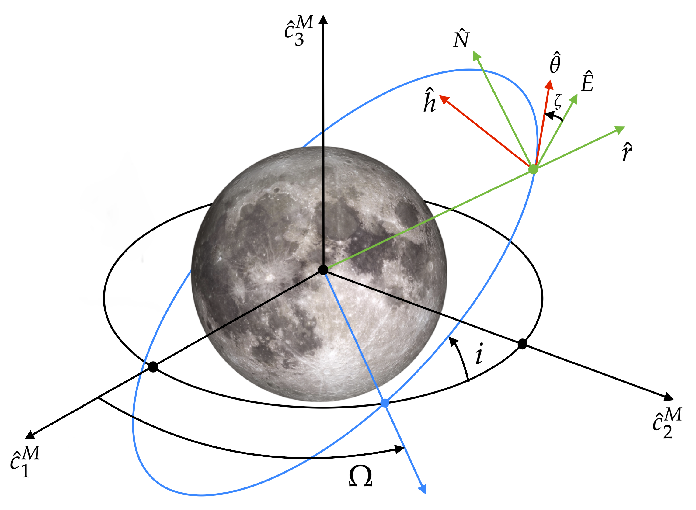
2. Orbit Dynamics
3. Nonlinear Orbit Control
3.1. Formulation of the Problem
3.2. Feedback Control Law
- ;
- (target set).
4. Numerical Simulations
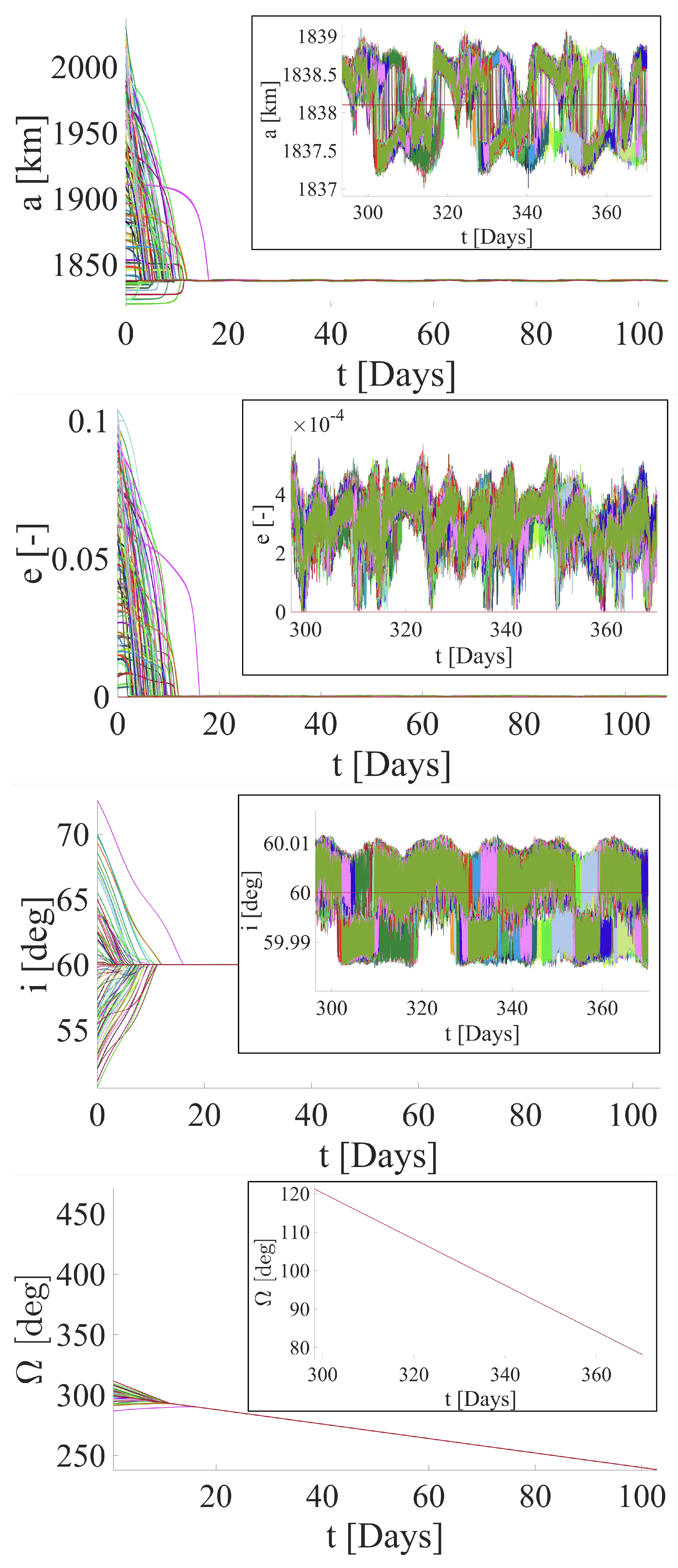
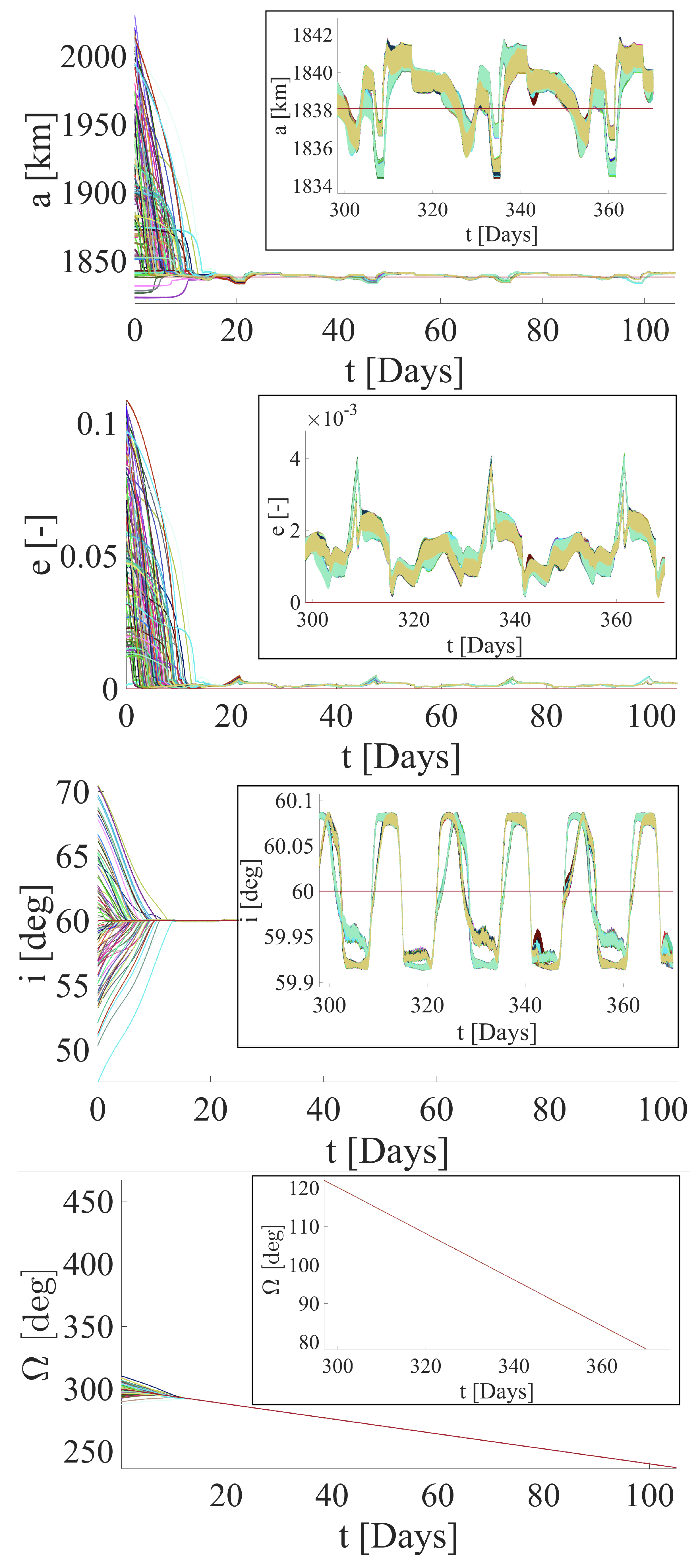
4.1. Target Orbit 1
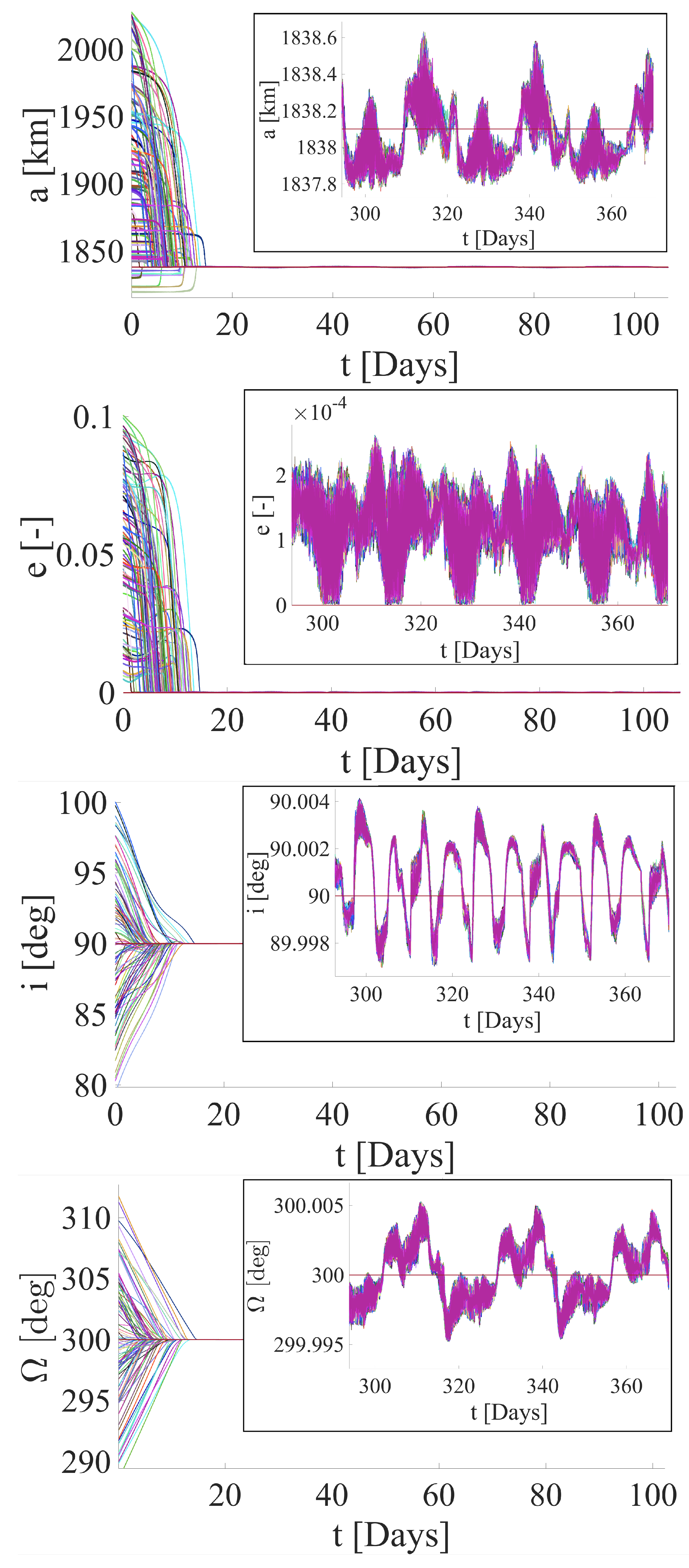
4.2. Target Orbit 2
5. Discussion of Results
6. Concluding Remarks
Author Contributions
Funding
Institutional Review Board Statement
Informed Consent Statement
Data Availability Statement
Conflicts of Interest
Abbreviations
| RAAN | Right Ascension of the Ascending Node |
| MCI | Moon Centered Inertial |
| LVLH | Local Vertical Local Horizontal |
| LH | Local Horizontal |
Appendix A. Planetary Data

| Body | |
|---|---|
| Sun | 132712440018 |
| Earth | 398600.4418 |
| Moon | 4902.7779 |
| Value | Value | ||
|---|---|---|---|
| 0.000203256369305959 | −2.2434487970911 × 10⁻⁶ | ||
| 8.59050334996568 × 10⁻⁶ | 4.61610568281654 × 10⁻⁶ | ||
| −9.8522886746674 × 10⁻⁶ | −6.7273906042203 × 10⁻⁶ | ||
| −1.3293051175382 × 10⁻⁵ | 5.54940421259954 × 10⁻⁶ | ||
| −2.2061158962342 × 10⁻⁵ | −4.6246357265911 × 10⁻⁶ | ||
| −9.4065451772204 × 10⁻⁶ | −1.4141219096004 × 10⁻⁶ | ||
| 1.51243401890736 × 10⁻⁵ | −1.6209625508441 × 10⁻⁶ | ||
| 3.89230799976237 × 10⁻⁶ | 1.29851648071154 × 10⁻⁶ | ||
| 5.14949783632897 × 10⁻⁶ | −1.7804783918105 × 10⁻⁶ | ||
| 9.1117958405472 × 10⁻⁶ | −1.4541586632206 × 10⁻⁶ | ||
| −1.4596672751979 × 10⁻⁶ | 2.1351214383094 × 10⁻⁶ | ||
| 5.70913026297742 × 10⁻⁶ | −1.9588420020059 × 10⁻⁶ | ||
| −4.7874115985482 × 10⁻⁶ | −1.3163362865652 × 10⁻⁶ | ||
| 2.97052872898108 × 10⁻⁶ | 1.26894455814441 × 10⁻⁶ | ||
| 1.75163995006724 × 10⁻⁶ | −1.0675927011228 × 10⁻⁶ | ||
| 2.34692497584258 × 10⁻⁶ | 1.92342072984345 × 10⁻⁶ | ||
| 1.21874850482553 × 10⁻⁶ | 1.0580049555114 × 10⁻⁶ |
| Value | Value | ||
|---|---|---|---|
| 0.000203256369305959 | 0.000415878398442979 | ||
| 8.59050334996568 × 10⁻⁶ | 0.20642811107848 | ||
| −9.8522886746674 × 10⁻⁶ | 0.16771320834929 | ||
| −1.3293051175382 × 10⁻⁵ | −0.0496398759987853 | ||
| −2.2061158962342 × 10⁻⁵ | 2.86012534158749 | ||
| −9.4065451772204 × 10⁻⁶ | −1.18630809022817 | ||
| 1.51243401890736 × 10⁻⁵ | −1.83532311833521 | ||
| 3.89230799976237 × 10⁻⁶ | −1.01434986302375 | ||
| 5.14949783632897 × 10⁻⁶ | −0.0229903684710072 | ||
| 9.1117958405472 × 10⁻⁶ | 0.11842818400149 | ||
| −1.4596672751979 × 10⁻⁶ | 1.89596195628963 |
Appendix B. Sensitivity Analysis with Respect to the Gravitational Model
| Parameter | Mean Value | Standard Deviation |
|---|---|---|
| [km] | 1838.04 | 5.18 × 10⁻¹ |
| 3.09 × 10⁻⁴ | 6.70 × 10⁻⁵ | |
| [deg] | 60.00 | 5.96 × 10⁻³ |
| [deg] | 1.56 × | 2.71 × 10⁻³ |
| Parameter | Mean Value | Standard Deviation |
|---|---|---|
| [km] | 1838.02 | 4.08 × 10⁻¹ |
| 3.25 × 10⁻⁴ | 6.71 × 10⁻⁵ | |
| [deg] | 60.00 | 5.75 × 10⁻³ |
| [deg] | 3.62 × | 2.84 × 10⁻³ |
| Parameter | Mean Value | Standard Deviation |
|---|---|---|
| [km] | 1838.01 | 3.82 × 10⁻¹ |
| 3.47 × 10⁻⁴ | 9.23 × 10⁻⁵ | |
| [deg] | 60.00 | 6.52 × 10⁻³ |
| [deg] | 1.01 × | 3.32 × 10⁻³ |
| Parameter | Mean Value | Standard Deviation |
|---|---|---|
| [km] | 1838.01 | 3.82 × 10⁻¹ |
| 3.47 × 10⁻⁴ | 9.13 × 10⁻⁵ | |
| [deg] | 60.00 | 6.75 × 10⁻³ |
| [deg] | 7.21 × | 3.40 × 10⁻³ |
| Parameter | Mean Value | Standard Deviation |
|---|---|---|
| [km] | 1838.04 | 4.95 × 10⁻¹ |
| 3.06 × 10⁻⁴ | 6.54 × 10⁻⁵ | |
| [deg] | 60.00 | 5.65 × 10⁻³ |
| [deg] | 1.62 × | 2.85 × 10⁻³ |
References
- Fuller, S.; Lehnhardt, E.; Zaid, C.; Halloran, K. Gateway Program Status and Overview. In Proceedings of the 72nd International Astronautical Congress, Dubai, United Arab Emirates, 25–29 October 2021. [Google Scholar]
- Lara, M. Design of long-lifetime lunar orbits: A hybrid approach. Acta Astronaut. 2011, 69, 186–199. [Google Scholar] [CrossRef]
- Nie, T.; Gurfil, P. Lunar frozen orbits revisited. Celest. Mech. Dyn. Astron. 2018, 130, 61. [Google Scholar] [CrossRef]
- Pontani, M.; Di Roberto, R.; Graziani, F. Lunar orbit dynamics and maneuvers for Lunisat missions. Acta Astronaut. 2018, 149, 111–122. [Google Scholar] [CrossRef]
- Singh, S.K.; Woollands, R.; Taheri, E.; Junkins, J. Feasibility of quasi-frozen, near-polar and extremely low-altitude lunar orbits. Acta Astronaut. 2020, 166, 450–468. [Google Scholar] [CrossRef]
- Liu, J.; Xu, B.; Li, C.; Li, M. Lifetime Extension of Ultra Low-Altitude Lunar Spacecraft with Low-Thrust Propulsion System. Aerospace 2022, 9, 305. [Google Scholar] [CrossRef]
- LaFarge, N.B.; Miller, D.; Howell, K.C.; Linares, R. Guidance for closed-loop transfers using reinforcement learning with application to libration point orbits. In Proceedings of the AIAA Scitech 2020 Forum, Orlando, FL, USA, 6–10 January 2020; p. 458. [Google Scholar]
- Hart, J.; King, E.; Miotto, P.; Lim, S. Orion GN&C architecture for increased spacecraft automation and autonomy capabilities. In Proceedings of the AIAA Guidance, Navigation and Control Conference and Exhibit, Honolulu, HI, USA, 16–21 August 2008; p. 7291. [Google Scholar]
- LaFarge, N.B.; Miller, D.; Howell, K.C.; Linares, R. Autonomous closed-loop guidance using reinforcement learning in a low-thrust, multi-body dynamical environment. Acta Astronaut. 2021, 186, 1–23. [Google Scholar] [CrossRef]
- Conway, B.A. A survey of methods available for the numerical optimization of continuous dynamic systems. J. Optim. Theory Appl. 2012, 152, 271–306. [Google Scholar] [CrossRef]
- Leomanni, M.; Bianchini, G.; Garulli, A.; Giannitrapani, A. A class of globally stabilizing feedback controllers for the orbital rendezvous problem. Int. J. Robust Nonlinear Control. 2017, 27, 4607–4621. [Google Scholar] [CrossRef]
- Kluever, C.A. Simple guidance scheme for low-thrust orbit transfers. J. Guid. Control. Dyn. 1998, 21, 1015–1017. [Google Scholar] [CrossRef]
- Gurfil, P. Nonlinear feedback control of low-thrust orbital transfer in a central gravitational field. Acta Astronaut. 2007, 60, 631–648. [Google Scholar] [CrossRef]
- Chang, D.E.; Chichka, D.F.; Marsden, J.E. Lyapunov-based transfer between elliptic Keplerian orbits. Discret. Contin. Dyn. Syst. Ser. B 2002, 2, 57–68. [Google Scholar] [CrossRef]
- Leeghim, H.; Cho, D.H.; Jo, S.J.; Kim, D. Generalized guidance scheme for low-thrust orbit transfer. Math. Probl. Eng. 2014, 2014, 407087. [Google Scholar] [CrossRef]
- Federici, L.; Benedikter, B.; Zavoli, A. Deep learning techniques for autonomous spacecraft guidance during proximity operations. J. Spacecr. Rocket. 2021, 58, 1774–1785. [Google Scholar] [CrossRef]
- Izzo, D.; Öztürk, E. Real-time guidance for low-thrust transfers using deep neural networks. J. Guid. Control. Dyn. 2021, 44, 315–327. [Google Scholar] [CrossRef]
- Capra, L.; Brandonisio, A.; Lavagna, M. Network architecture and action space analysis for deep reinforcement learning towards spacecraft autonomous guidance. Adv. Space Res. 2023, 71, 3787–3802. [Google Scholar] [CrossRef]
- Petropoulos, A.E. Refinements to the Q-Law for the Low-Thrust Orbit Transfers. In Proceedings of the 15th AAS/AIAA Space Flight Mechanics Conference, Copper Mountain, CO, USA, 23–27 January 2005. [Google Scholar]
- Narayanaswamy, S.; Damaren, C.J. Equinoctial Lyapunov control law for low-thrust rendezvous. J. Guid. Control. Dyn. 2023, 46, 781–795. [Google Scholar] [CrossRef]
- Peterson, J.T.; Arya, V.; Junkins, J.L. Connecting the Equinoctial Elements and Rodrigues Parameters: A New Set of Elements. J. Guid. Control. Dyn. 2023, 46, 1726–1744. [Google Scholar] [CrossRef]
- Pontani, M.; Pustorino, M. Nonlinear Earth orbit control using low-thrust propulsion. Acta Astronaut. 2021, 179, 296–310. [Google Scholar] [CrossRef]
- Pontani, M.; Teofilatto, P. Deployment strategies of a satellite constellation for polar ice monitoring. Acta Astronaut. 2022, 193, 346–356. [Google Scholar] [CrossRef]
- Pontani, M.; Pustorino, M. Low-Thrust Lunar Capture Leveraging Nonlinear Orbit Control. J. Astronaut. Sci. 2023, 70, 28. [Google Scholar] [CrossRef]
- Battin, R.H. An Introduction to the Mathematics and Methods of Astrodynamics; AIAA: Reston, VA, USA, 1999. [Google Scholar]
- Giorgi, S. Una Formulazione Caratteristica del Metodo Encke in Vista Dell’Applicazione Numerica; Università di Roma, Scuola di Ingegneria Aerospaziale: Rome, Italy, 1964. [Google Scholar]
- Konopliv, A.; Asmar, S.; Carranza, E.; Sjogren, W.; Yuan, D. Recent gravity models as a result of the Lunar Prospector mission. Icarus 2001, 150, 1–18. [Google Scholar] [CrossRef]
- Curtis, H. Orbital Mechanics for Engineering Students; Butterworth-Heinemann: Oxford, UK, 2013. [Google Scholar]
- Wolfram Mathematica. 2023. Available online: https://www.wolfram.com/mathematica/ (accessed on 9 January 2024).


| Orbital Element | [deg] | [deg] |
|---|---|---|
| Target orbit 1 | 60 | 300 |
| Target orbit 2 | 90 | 300 |
| Parameter | Mean Value | Standard Deviation |
|---|---|---|
| [km] | 1837.96 | 4.83 · 10−2 |
| 3.20 · 10−4 | 4.15 · 10−6 | |
| [deg] | 59.99 | 3.38 · 10−5 |
| [deg] | 4.87 · | 9.15 · 10−5 |
| Final Mass Ratio | 0.625 | 5.29 · 10−3 |
| Parameter | Mean Value | Standard Deviation |
|---|---|---|
| [km] | 1838.83 | 3.38 · 10−2 |
| 1.54 · 10−3 | 4.34 · 10−6 | |
| [deg] | 59.99 | 8.47 · 10−6 |
| [deg] | 8.63 · | 8.63 · 10−4 |
| Final Mass Ratio | 0.890 | 2.94 · 10−3 |
| Parameter | Mean Value | Standard Deviation |
|---|---|---|
| [km] | 1838.33 | 3.37 · 10−3 |
| 3.11 · 10−4 | 1.80 · 10−6 | |
| [deg] | 90.00 | 2.45 · 10−7 |
| [deg] | 1.81 · | 3.68 · 10−7 |
| Final Mass Ratio | 0.661 | 1.50 · 10−3 |
| Parameter | Mean Value | Standard Deviation |
|---|---|---|
| [km] | 1837.34 | 1.61 · 10−1 |
| 2.31 · 10−3 | 6.41 · 10−5 | |
| [deg] | 90.00 | 7.43 · 10−7 |
| [deg] | 4.42 · | 2.12 · 10−6 |
| Final Mass Ratio | 0.911 | 3.56 · 10−3 |
Disclaimer/Publisher’s Note: The statements, opinions and data contained in all publications are solely those of the individual author(s) and contributor(s) and not of MDPI and/or the editor(s). MDPI and/or the editor(s) disclaim responsibility for any injury to people or property resulting from any ideas, methods, instructions or products referred to in the content. |
© 2024 by the authors. Licensee MDPI, Basel, Switzerland. This article is an open access article distributed under the terms and conditions of the Creative Commons Attribution (CC BY) license (https://creativecommons.org/licenses/by/4.0/).
Share and Cite
Leonardi, E.M.; Pontani, M.; Carletta, S.; Teofilatto, P. Low-Thrust Nonlinear Orbit Control for Very Low Lunar Orbits. Appl. Sci. 2024, 14, 1924. https://doi.org/10.3390/app14051924
Leonardi EM, Pontani M, Carletta S, Teofilatto P. Low-Thrust Nonlinear Orbit Control for Very Low Lunar Orbits. Applied Sciences. 2024; 14(5):1924. https://doi.org/10.3390/app14051924
Chicago/Turabian StyleLeonardi, Edoardo Maria, Mauro Pontani, Stefano Carletta, and Paolo Teofilatto. 2024. "Low-Thrust Nonlinear Orbit Control for Very Low Lunar Orbits" Applied Sciences 14, no. 5: 1924. https://doi.org/10.3390/app14051924