A Bearing Fault Diagnosis Method Based on Improved Transfer Component Analysis and Deep Belief Network

Abstract

Domain adaptation can handle data distribution in different domains and has been successfully applied to bearing fault diagnosis under variable working conditions. However, most of these methods ignore the influences of noise and data distribution discrepancy on marking pseudo labels. Additionally, most domain adaptive methods require a large amount of data and training time. To overcome the aforementioned challenges, firstly, sample rejection and pseudo label correction using K-means (SRPLC-K-means) were developed and explored to filter the noisy samples and correct the pseudo labels to obtain pseudo labels with higher confidence. Furthermore, a bearing fault diagnosis method based on the improved transfer component analysis and deep belief network is proposed, which can achieve subdomain adaptation and improve the compactness of the samples, leading to a complete bearing fault diagnosis under variable working conditions that is faster and more accurate. Finally, the results of the comparative tests confirmed that the proposed method could boost the average accuracy of 0.73%, 0.99%, and 5.55% in the three tests than the state-of-the-art methods, respectively. Moreover, the comparison of the time required for a fault diagnosis using different methods shows that compared to the end-to-end models, the proposed method reduces the time required by 594.9 s and 1431.6 s, respectively.

1. Introduction

Bearings are widely used in rotating mechanical equipment, such as wind turbines, motor rotations, and rollers. When many rotating machineries operate in harsh environments, their bearings are prone to faults, such as friction, oxidation, wear, pitting, and fracture. A faulty bearing is likely to cause an impact at the fault point, increase friction, and cause damage to rotating mechanical equipment, ultimately leading to shut down and even the overall paralysis of the mechanical equipment system, resulting in huge economic losses.

Traditional bearing fault diagnoses mainly analyze the fault features of bearings from the perspective of signal feature extraction and then combine them with classifiers to identify fault types. Common time-frequency analysis methods include empirical mode decomposition [1], and wavelet transform [2,3]. Common fault identification methods include convolutional neural networks [4], fuzzy neural networks [5], support vector machines [6], and random forests [7]. Empirical mode decomposition is suitable for processing nonlinear and nonstationary signals, but it has stability and computational complexity issues. Wavelet transform is suitable for capturing the time-frequency characteristics of signals, but it has limitations in handling non-stationary signals. Support vector machines and random forests are susceptible to noise. Convolutional neural networks and fuzzy neural networks are prone to computational complexity and long training times. References [8,9,10,11] introduced deep belief networks (DBNs) into bearing fault diagnoses, further improving the accuracy of fault recognition. Unsupervised domain adaptation (UDA) [12,13,14,15] has been applied to fault diagnoses, improving the fault diagnosis of variable working conditions. The maximum mean discrepancy (MMD) [16,17] has been used to align the data distribution of samples between different domains to achieve UDA, which has attracted much attention from scholars. However, UDA can only globally align the global data distribution between two domains and cannot capture more fine-grained information. Reference [18] proposed local maximum mean discrepancy (LMMD), which can align data distributions of the same category and achieve unsupervised subdomain adaptation (USDA). Reference [19] proposed clustering domain adaptation, which minimizes the nearest neighbor distance between similar samples and maximizes the distance between the cluster centers of samples within the same domain. The adaptive clustering domain further improves the accuracy of fault diagnoses under variable operating conditions [20]. The prerequisite for achieving subdomain adaptation is to obtain reliable labels in the target domain. Reference [21] used feature transferability and output probability similarity to mark the unlabeled target domains with pseudo labels. Reference [22] assisted in achieving USDA by labeling the target domain with pseudo labels. The principle of labeling pseudo labels is to use the classifier trained on the source domain data to label them. The accuracy of pseudo labels is influenced by the discrepancies in data distribution and sample noise. Relying solely on LMMD as the objective function for subdomain adaptation easily leads to local optima and the complexification of the mapping matrix. The implementation of the above methods is an end-to-end model that directly inputs raw data into a neural network for feature extraction and fault type recognition [21]. The end-to-end model utilizes a large-scale neural network to extract abstract features from raw data. However, using neural networks to extract features from raw data requires a significant amount of training time and data and is sensitive to noise.

In the industry, the distribution of data is greatly influenced by the degree of damage, bearing type, noise, and variable working conditions. It is difficult to reduce the impact of varying degrees of damage and noise using domain adaptation. The impact will reduce the accuracy of pseudo labels. To minimize the impact, noise reduction processing is required before feature extraction. Based on this, this article proposes a bearing fault diagnosis model using an improved transfer component analysis and deep belief network (ITCA-DBN) and a method named samples rejection and pseudo label correction using K-means (SRPLC-K-means). ITCA-DBN is a segmented data processing model that requires manual feature extraction and fault diagnosis. Compared to end-to-end models, segmented data processing models require less time for feature extraction.

The proposed ITCA uses LMMD instead of MMD and adds a divergence factor. LMMD solves the problem of data distribution discrepancies within the same category between different domains. The divergence factor can be used to measure the sample compactness of a category. Improving the intraclass clustering of samples and reducing the impact of noise can improve the accuracy of classification. When there are significant discrepancies in the data distribution, the accuracy of pseudo labels sharply decreases, which greatly affects the transfer ability of the model. To improve the accuracy of pseudo labels in the target domain, K-means clustering is used to correct the pseudo labels and remove the edge samples. Finally, based on multiple experimental comparisons, it was verified that the proposed method could complete bearing fault diagnoses under variable working conditions in a short time and with high accuracy.

The contributions are presented as follows:

• The divergence factor is proposed to measure the compactness of samples within a category. Considering subdomain adaptation and divergence factors aims to improve the TCA, reducing subdomain discrepancies and increasing sample compactness;
• A simple method named SRPLC-K-means was designed to filter the noisy samples and correct the pseudo labels. The experimental results have verified that the SRPLC-K-means method is helpful in overcoming the issue of false pseudo labels;
• The experimental results on Case Western Reserve University and underground drum motor bearing datasets have demonstrated that the proposed method can reduce the time required for a fault diagnosis and increase accuracy.

The rest of this paper is presented as follows: The fundamental theories of the TCA, subdomain adaptation, and DBN are illustrated in Section 2. Section 3 introduces the ITCA and SRPLC-K-means in detail. In Section 4, the experiments are detailed, which include the accuracy, visualization, and time required for a fault diagnosis on the Case Western Reserve University case and underground drum motor bearing datasets. Finally, the overall work and future research directions are summarized in Section 5.

2. Basic Theory

2.1. Transfer Component Analysis

TCA is a transfer learning method based on domain adaptation [23] proposed by Pan et al. [24]. The principle is to utilize the transferability of the features between domains, map the source and target domains to a lower dimensional shared feature space, and search for common transfer components for learning [25]. The mapping process of TCA uses MMD as the metric criterion, which greatly reduces the distribution discrepancy between the source domain and the target domain while retaining its internal attributes so that the edge distribution probability density and conditional probability density of the mapped data source domain and target domain are equal. TCA plays an important role in cross-domain transfer learning, where there is a significant discrepancy in the data distribution between the source and target domains. Equation (1) is the mathematical expression for MMD.

$$D_H(X_s,X_t)={‖\frac{1}{n_s}{\displaystyle \sum _{i=1}^{n_s}\varphi (x_i)-\frac{1}{n_t}{\displaystyle \sum _{j=1}^{n_t}\varphi (x_j)}}‖}_H^2$$

(1)

where, $X_s$ and $X_t$ are the sample sets of the source domain and target domain, $n_s$ and $n_t$ are the number of samples in the source domain and target domain, respectively. The variable $\varphi$ is the mapping function that satisfies two probability distributions, $\varphi (x_i)$ and $\varphi (x_j)$, minimizing MMD, and ${‖\cdot ‖}_H^2$ is the reproducing kernel Hilbert space (RKHS) norm. If MMD is directly optimized, the mapping function is prone to falling into local optima. Therefore, regularization is introduced to constrain the complexity of the kernel function matrix $K$ and the mapping matrix $L$. Equation (1) is simplified as follows:

$$D_H(X_s,X_t)=tr(KL)$$

(2)

where $tr(\cdot )$ is the trace of the matrix. The calculation formula for the kernel function matrix $K$ is shown in Equation (3), and the calculation for the mapping matrix $L$ is shown in Equation (4).

$$K=\left[\begin{array}{cc}{K}_{s,s}& K_{s,t}\\ K_{t,s}& K_{t,t}\end{array}\right]\in {ℝ}^{(n_s+n_t)\times (n_s+n_t)}$$

(3)

where, $K_{s,s}$, $K_{s,t}$, $K_{t,s}$, $K_{t,t}$ represent the kernel functions of the source domain, cross domain, and target domain in the mapped space, respectively.

$$L_{ij}=\left\{\begin{array}{ll}\frac{1}{n_s^2}\hfill & x_i,x_j\in X_s\hfill \\ \frac{1}{n_t^2}\hfill & x_i,x_j\in X_t\hfill \\ -\frac{1}{n_s{n}_s}\hfill & \mathrm{otherwise}\hfill \end{array}\right.$$

(4)

To further simplify the calculation, the kernel function matrix K is mapped to an m-dimensional space, and a low-dimensional matrix $W$ is introduced, and the formula is as follows:

$$\tilde{K}=(K{K}^{-1/2}\tilde{W})({\tilde{W}}^T{K}^{-1/2}K)=KW{W}^{T}K$$

(5)

where $\tilde{K}$ is a temporary variable, $W=K^{-1/2}\tilde{W}$ and $W^{T}KHKW$ represent the variance of the mapping sample, and $H=I_{n_s+n_t}-[1/(n_s+n_t)]I{I}^T$ represents the central matrix, $I\in {ℝ}^{(n_s+n_t)\times (n_s+n_t)}$. The ultimate optimization goal of TCA is shown in Equation (6):

$${\min }_W=tr\left(W^{T}KLKW\right)+u\times tr(W^{T}W)$$

(6)

where $u>0$ is the equilibrium hyperparameter.

The implementation steps of TCA are as follows: input the feature sample sets $X_s$ and $X_t$ of the source domain and target domain, then select the kernel function to calculate the matrix $K$, map the matrix $L$ and matrix $H$, and finally output the new feature sample sets $T_s$ of the source domain and $T_t$ of the target domain after distribution alignment.

2.2. Subdomain Adaptation

The purpose of global domain adaptation and subdomain adaptation is to reduce distribution discrepancies. Subdomain adaptation focuses on reducing the distribution discrepancies of data within the same category between different domains. The difference between global domain adaptation and subdomain adaptation is shown in Figure 1. The left side of Figure 1 describes the distribution of the original data between the target domain and the source domain, the upper right part describes the global domain adaptation and the lower right part describes the subdomain adaptation. Although the global domain adaptation alignment aligns the distribution of data in two domains, there are significant discrepancies in the distribution of the same type of data between different domains, leading to type aliasing. Subdomain adaptation aligns the data distribution of two domains for each type, which can avoid type aliasing.

MMD is used to measure the global data distribution discrepancies between two domains, while LMMD is usually used to measure the distribution discrepancies between two subdomains. The mathematical expression of LMMD is shown in Equation (7).

$$L{D}_H(X_s,X_t)=\frac{1}{C}{\displaystyle \sum _{m=1}^C{‖\frac{1}{n_s^m}{\displaystyle \sum _{i=1}^{n_s^m}\varphi (x_i^m)-\frac{1}{n_t^m}{\displaystyle \sum _{j=1}^{n_s^m}\varphi (x_j^m)}}‖}_H^2}$$

(7)

where $n_s^m$ and $n_t^m$ represent the number of samples for category $m$ in the source domain and target domain, respectively, and $C$ represents the number of labels.

2.3. Deep Belief Networks

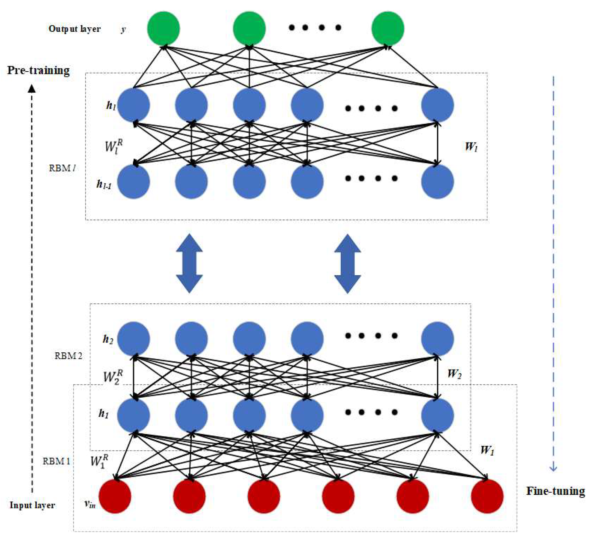
Deep belief networks consist of some restricted Boltzmann machines [26] (RBMs) stacked sequentially. The learning process of DBNs is divided into unsupervised learning and supervised learning. Unsupervised learning, also known as pre-training, is implemented using the contrastive divergence [27] (CD) algorithm. Supervised learning is implemented using the backpropagation (BP) network in the last layer, which is used to fine-tune the weight parameters of unsupervised learning. The mechanism of the DBN is to use multi-layer RBM to extract and process the features of the target, and then use a classifier for classification. The structures of DBN are shown in Figure 2.

In the DBNs, $v=v_1,v_2,\cdots v_n$ and $h=h_1,h_2,\cdots h_n$ denote the states of the visible variables and hidden variables, respectively. $W^R$ denotes a $m\times n$ weight matrix connecting the neurons between the visible and hidden layers. The joint probability distribution $P(v,h;\theta )$ and the energy function $E(v,h;\theta )$ between the hidden and visible layers of the RBM are shown in Equations (8) and (9). The purpose of the greedy layer-by-layer training is to maximize the joint probability distribution.

$$P(v,h;\theta )=\frac{1}{Z}{e}^{-E(v,h;\theta )}$$

(8)

$$E(v,h;\theta )=-{\displaystyle \sum _{i=1}^m{a}_i{v}_i-}{\displaystyle \sum _{j=1}^n{b}_j{h}_j-{\displaystyle \sum _{i=1}^m{\displaystyle \sum _{j=1}^n{v}_i}{w}_{ij}^R{b}_j}}$$

(9)

where $Z$ is the partition function (normalization factor), $w_{ij}^R$ is the connecting weight of the RBM, parameter set $\theta =(W^R,a,b)$ composed of $w_{ij}^R$, $a_i$ and $b_j$, $a_i$ and $b_j$ are the bias of the visible and hidden neurons, respectively. The update of $\theta$ is shown in Equation (10).

$${\theta }_{l+1}={\theta }_l+\eta \Delta {\theta }_l$$

(10)

where $\eta$ is the learning rate.

The backpropagation of the DBN belongs to supervised learning implemented using the BP network. The cross-entropy loss [26] can serve as the objective function for fine-tuning all layers in the BP network, as shown in Equation (11).

$$E=-\frac{1}{N}{\displaystyle \sum _{i=1}^N{y}_i^k\log p_i^k}$$

(11)

where $N$ represents the number of samples, $y_i^k$ represents the true label of the $i$th sample as $k$, and $p_i^k$ is the predictive probability that the $i$th sample belongs to category $k$.

3. Proposed Method

3.1. Improved Transfer Component Analysis

3.1.1. Dispersion Factor

Any sample is mixed with noise to a greater or lesser extent. When feature transfer occurs, noisy features are easily amplified, causing the mapped samples to diverge. It is necessary to improve the intraclass aggregation of the mapped samples to reduce the impact of noise and facilitate classification. Based on this, according to the idea of variance, the dispersion factor $S$ is proposed to measure the aggregation degree of the intraclass samples. The calculation of the dispersion factor $S$ is shown in Equation (12).

$$S=\frac{1}{n}{\displaystyle \sum _{j=1}^C{\displaystyle \sum _{i=1}^{m_j}{d}_i^j}}$$

(12)

where $n$ represents the total number of samples, $C$ represents the number of categories, $m_j$ represents the number of samples in class j, and $d_i^j$ represents the Euclidean distance between the ith sample in class j and the cluster center of the corresponding category. The calculation of the Euclidean distance is shown in Equation (14).

3.1.2. Improved Transfer Component Analysis

TCA achieves domain adaptation by aligning the global distribution between the target domain and the source domain but lacks consideration for the same category between different domains, resulting in suboptimal transfer learning performance. Subdomain adaptation can align data distributions of the same category between different domains. Therefore, for the fault diagnosis of bearings with different types of variable working conditions, LMMD is used to reduce the data distribution of the same fault type between different working conditions and bearing types and improve classification accuracy. When TCA maps the feature vectors of two domains to a shared feature space, the original distribution of the data mixed with noise will cause the mapped samples to diverge. So, it is necessary to reduce the intra-class divergence and improve class recognition. Therefore, this article proposes an improved transfer component analysis (ITCA) using LMMD instead of MMD, and the dispersion factor is considered in the objective function. The objective function of ITCA combining Equations (6), (7), and (12) is shown in Equation (13):

$${\min }_{\mathrm{ITCA}}=L{D}_H(X_s,X_t)+u\times \mathrm{tr}(W^{T}W)+\lambda S$$

(13)

where $u$ and $\lambda$ are the trade-off hyper-parameters.

3.2. SRPLC-K-Means

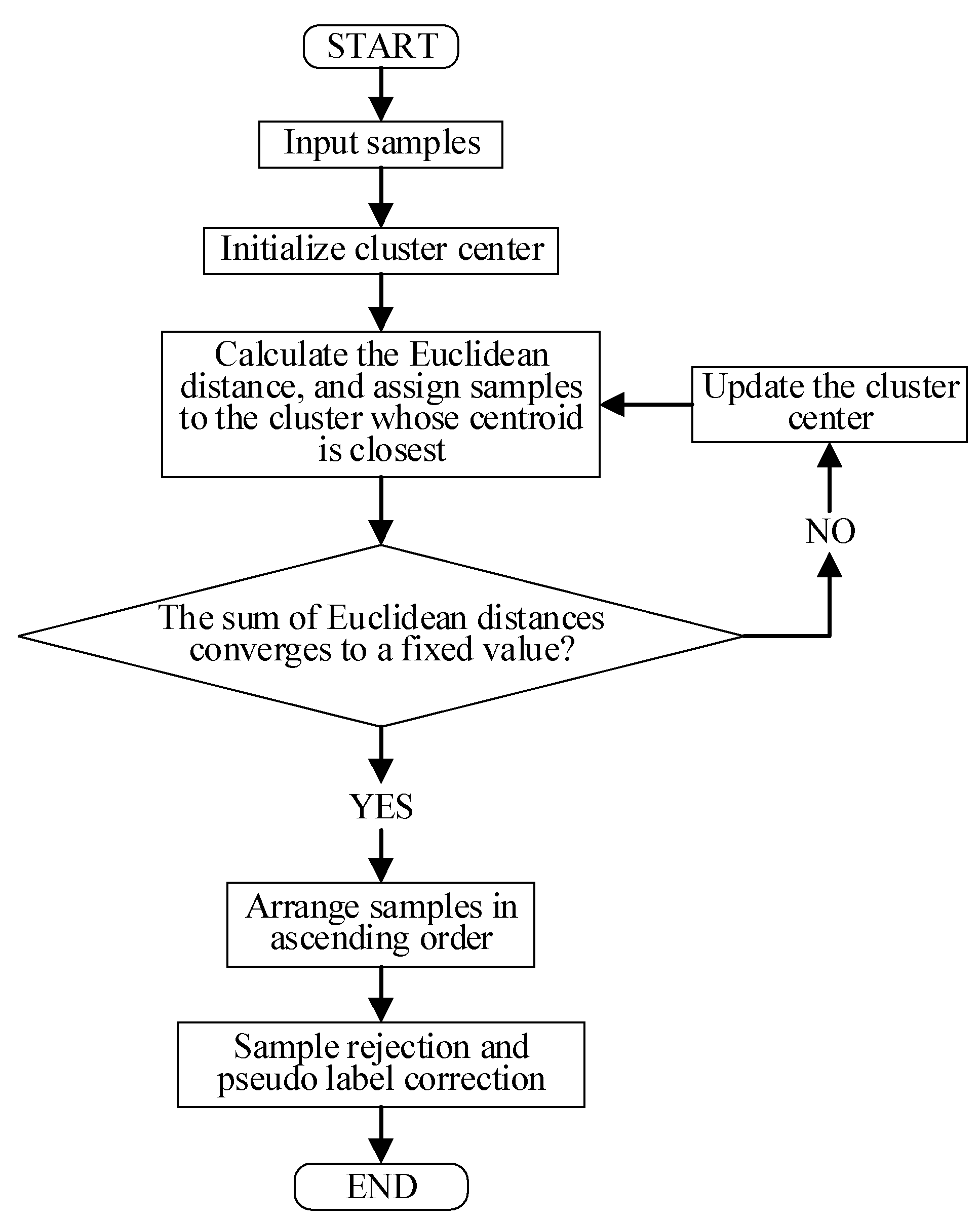
The prerequisite for achieving subdomain adaptation is that the label of the target domain is known. However, the target domain is an unlabeled set consisting of feature vectors. Some scholars have used pseudo labels to mark the target domain [18], but the model that marks pseudo labels is obtained through suboptimal training [28]. However, the accuracy of pseudo labels greatly affects the model’s alignment of data distribution in different fields. The existing noise in the samples and distribution discrepancies in the original data are the reasons why the accuracy is poor. Filtering noisy samples and correcting erroneous pseudo labels are necessary for unsupervised domain adaptation. Therefore, this article proposes the SRPLC-K-means method to obtain the higher confident pseudo labels. SRPLC-K-means requires the use of K-means for clustering and arranging the distance between the samples and cluster centers. K-means clustering is an unsupervised clustering method that measures the distance between the samples using the Euclidean distance. The flowchart of SRPLC K-means is shown in Figure 3, and its process is as follows:

• Randomly select k initial cluster centers $(z_1,z_2,\dots ,z_k)$ from N samples;
• Calculate the Euclidean distance from each sample $x^s$ to the nearest cluster center $z_j$ and assign the sample $x^s$ to the cluster where $z_j$ is located. The calculation of the Euclidean distance from the center is shown in Equation (14);

  $$d=\sqrt{{{\displaystyle {\sum }_{i=1}^n(x_i^s-x_i^z)}}^2}$$

  (14)

  where $x_i^z$ is the coordinates of the cluster center, $x_i^s$ is the coordinates of the sample, and n is the feature dimension of the sample;
• Update the cluster center and recalculate the distance between each sample and the cluster center it belongs to;
• Repeat steps 2 and 3 until the sum of the Euclidean distances from all the samples to their respective cluster centers converges to a fixed value;
• Arrange the samples of each cluster in ascending order based on their Euclidean distance from the cluster center they belong to;
• Reserve the samples in the top d% of the sequence number. Adopting the idea of the minority obeying the majority, modify the pseudo labels of minority classes in the new sample set to those of majority classes.

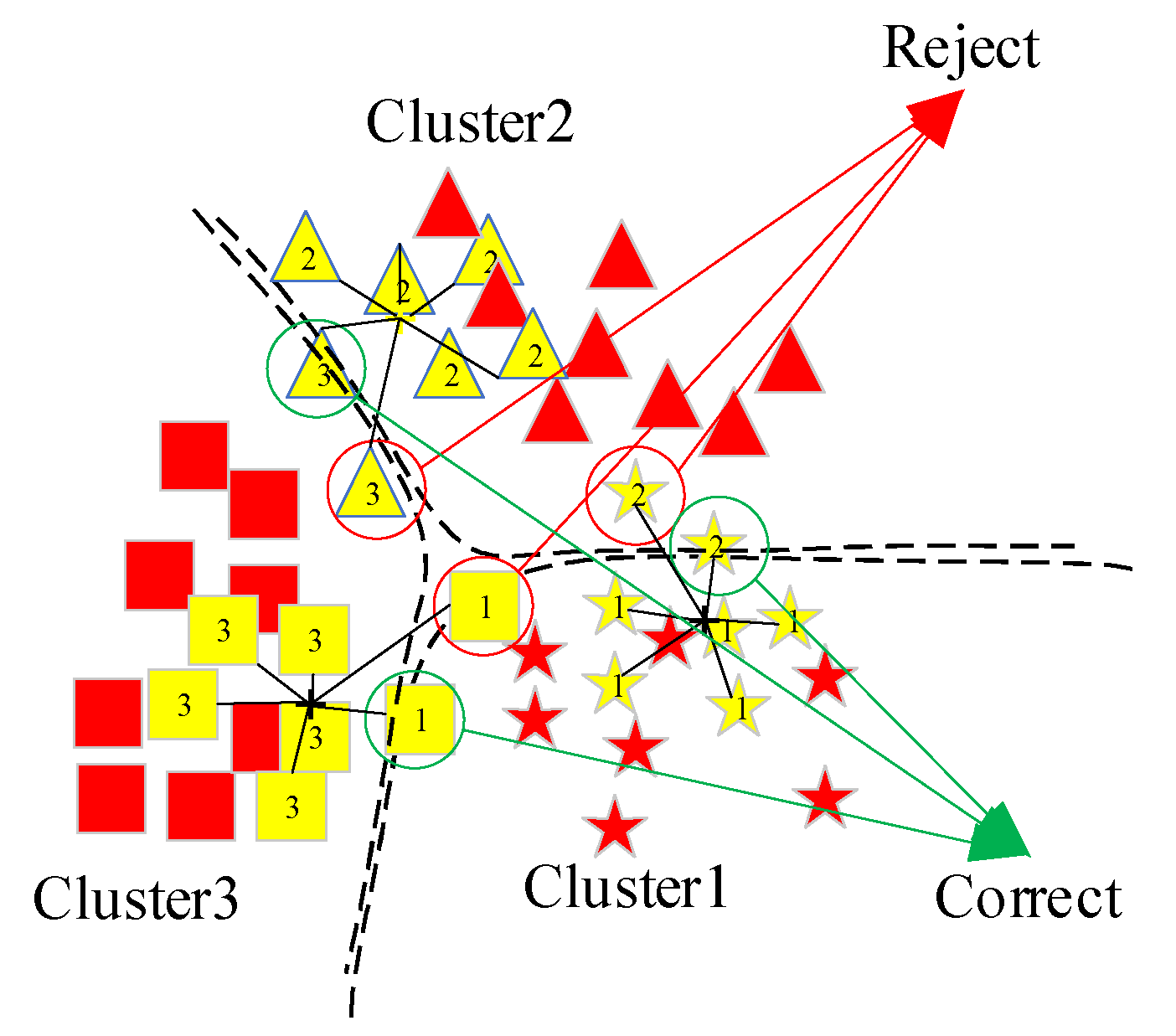
The pseudo labels are marked by classifier labels trained on source domain data, so they are mainly affected by discrepancies in data distribution and noise. The classification using K-means clustering is mainly affected by noise. When using K-means clustering for classification, the noise of the samples near the cluster center is low, so that the labels of the samples have higher confidence. Edge samples are prone to category aliasing and misjudging due to their heavily existing noise and being far from the cluster center. Therefore, this article proposes filtering and correction operations to remove the samples affected by noise and correct the false labels caused by the discrepancies in the data distribution. As shown in Figure 4, red and yellow represent the source domain and target domain samples, respectively. The numbers marked on the samples represent their pseudo labels, and the black cross symbol represents the cluster center of the target domain. The samples inside the red circle are those that are far from the cluster center of the target domain and have been mislabeled. They contain significant noise and are close to other categories, rendering them difficult to distinguish and should be filtered. The samples inside the green circle are those that are close to the cluster center of the target domain but have been mislabeled. They contain less noise, but their data distribution is similar to other categories in the source domain. Due to the small number of samples in the target domain, its pseudo labels should be corrected.

3.3. The Fault Diagnosis Model of the Proposed Method

The bearing fault diagnosis method based on the improved transfer component analysis and deep belief network mainly consists of three parts: feature extraction, data processing, and fault classification. The proposed method has two core points. One is to use ITCA to reduce the data distribution discrepancies of the same fault type between the source domain and the target domain, aligning the subdomain data distribution of the two domains. Another approach is to use K-means clustering to remove interclass edge samples and correct the pseudo labels.

Firstly, wavelet packets are used to denoise and extract the features from the source and target the domain signals. We then use the source domain samples as the training set and divide the target domain samples into a validation set and a testing set. Then, we use a classifier trained in the source domain to label the unlabeled validation sets with pseudo labels. Then, we use K-means clustering to classify the validation set and calculate the distribution of the pseudo labels for each cluster sample. Adopting the idea of the minority obeying the majority, the pseudo labels of the samples in the top d% of the distance from the cluster center are corrected to the one with the most pseudo labels in that cluster. Then, we perform ITCA processing on the training and validation sets and output the feature vectors after dimensionality reduction. Then, we input the training set samples after dimensionality reduction into the DBN for pretraining, and use the validation set samples after dimensionality reduction for fine-tuning the DBN. Finally, the optimal mapping relationship is applied to the test set samples, and the trained DBN model is used to classify the faults in the test set after dimensionality reduction. The specific implementation steps of the fault diagnosis method proposed are shown below, and the fault diagnosis flow chart of the proposed method is shown in Figure 5.

Step 1: Denoising and feature extraction. We performed wavelet packet decomposition, denoising, and reconstruction on the bearing data. Then, we extracted multiple time-frequency features to form a feature vector;

Step 2: Allocation of the datasets. All the source domain samples were used as the training set, a small number of unlabeled target domain samples were randomly grabbed as the validation set, and a portion of the target domain samples were taken as the testing set;

Step 3: Marking the pseudo labels. We used the DBN trained on the training set to mark the pseudo labels to the validation set;

Step 4: Sample filtering and pseudo label correction. We filtered the edge samples and corrected the pseudo labels on the validation set using K-means clustering;

Step 5: We performed ITCA mapping on the training and validation set samples;

Step 6: We trained a new DBN using the training and validation sets after dimensionality reduction;

Step 7: Using the mapping function obtained in step 5, we processed the test set samples;

Step 8: We input the testing set samples after dimensionality reduction into the DBN trained in step 6 and output the diagnostic results.

4. Experimental Analysis and Verification

4.1. Preparation of the Experimental Data

4.1.1. Introduction of the Dataset

This paper uses the motor rolling bearing dataset from Case Western Reserve University [29] (CWRU) to validate the proposed method. This dataset includes three types of faults: an outer ring fault, rolling element fault, and inner ring fault, as well as the normal types. Each type contains vibration signals of bearings with different damage sizes, speeds, and load faults. The CWRU bearing testing equipment consists of a 2 HP torque motors, sensors, power testers, etc. The drive end bearing model is SKF6205, and the fan end bearing model is SKF6203 (SKF, Yokohama, Japan).

The CWRU bearing test collected data from various working conditions. There are four different dimensions of damage size: 0.356 mm, 0.533 mm, and 0.714 mm. There are four types of loads: 0 HP, 1 HP, 2HP, and 3HP. There are four types of rotational speeds: 1797 r/min, 1772 r/min, 1750 r/min, and 1730 r/min. The health status includes the normal state, inner ring fault, rolling element fault, and outer ring fault. Specific information on the bearing dataset is shown in

Table 1. Bearing dataset.

Types of Bearing	Working Conditions	Rotational Speeds	Loads	Health Status
SKF6205	A	1797 r/min	0 HP	Normal state Inner ring fault Rolling element fault Outer ring fault
	B	1772 r/min	1 HP
	C	1750 r/min	2 HP
	D	1730 r/min	3 HP
SKF6203	E	1797 r/min	0 HP
	F	1772 r/min	1 HP
	G	1750 r/min	2 HP
	H	1730 r/min	3 HP

.

4.1.2. Feature Extraction

Since the denoising and feature extraction of the signals can affect the fault diagnosis of the model, wavelet packet decomposition, threshold filtering, and signal reconstruction on the data were performed to remove the noise. Then, the time-frequency features of the reconstructed signal are extracted, forming a vector Z. The Morlet wavelet was suitable for decomposing the bearing vibration signals [30], thus, it was selected as the wavelet basis function in this section.

To better highlight the fault information of the motor bearings, eight obvious features of faulty bearings were extracted: the mean value, standard deviation, root mean square, pulse index, margin index, skewness index, kurtosis index, and waveform entropy. These features reflect the various characteristics of the vibration signals and demonstrate robust discriminative ability and stability across different fault conditions. Then, the above time-frequency features were combined as the feature vector Z. The expressions for the above features are shown in

Table 2. Expressions of the time domain features.

Name	Definition	Name	Definition
Average	$\overline{x}=\frac{1}{N}{\displaystyle {\sum }_{i=1}^N{x}_i}$	Standard deviation	$S=\sqrt{\frac{1}{N}{\displaystyle {\sum }_{i=1}^N{(x_i-\overline{x})}^2}}$
Margin index	$C_e=\frac{x_{rms}}{\overline{x}}$	Skewness index	$C_w=\frac{1}{N}{\displaystyle {\sum }_{i=1}^N(\frac{\left|x_i\right|-\overline{x}}{x_{rms}}}{)}^3$
Root mean square	$x_{rms}=\sqrt{\frac{1}{N}{\displaystyle {\sum }_{i=1}^N{x_i}^2}}$	Kurtosis index	$C_q=\frac{1}{N}{\displaystyle {\sum }_{i=1}^N(\frac{\left|x_i\right|-\overline{x}}{x_{rms}}}{)}^4$
Pulse index	$C_f=\frac{x_p}{\overline{x}}$	Waveform entropy	$C_q=\frac{1}{N}{\displaystyle {\sum }_{i=1}^N{x}_i\log x_i}$

.

We took 120,000 consecutive sampling points from all datasets A, B, C, D, E, F, G, and H, and divided them into 400 samples according to the time series. Each sample contained 300 consecutive sampling points. Then, we extracted eight features for each sample based on the expressions in Table 2 and formed a vector.

4.2. Test Ⅰ

The purpose of this experiment was to test the performance of the ITCA-DBN model for a fault diagnosis under variable working conditions. There were a total of six tasks of cross-working condition fault diagnoses in this experiment, which were A → B, A → C, A → D, B → C, B → D, and C → D. We took all the samples from the source domain dataset as the training set, randomly selected 50 samples from each state type in the target domain as the validation set, and then randomly selected 120 samples from each state type in the target domain as the testing set for the target domain.

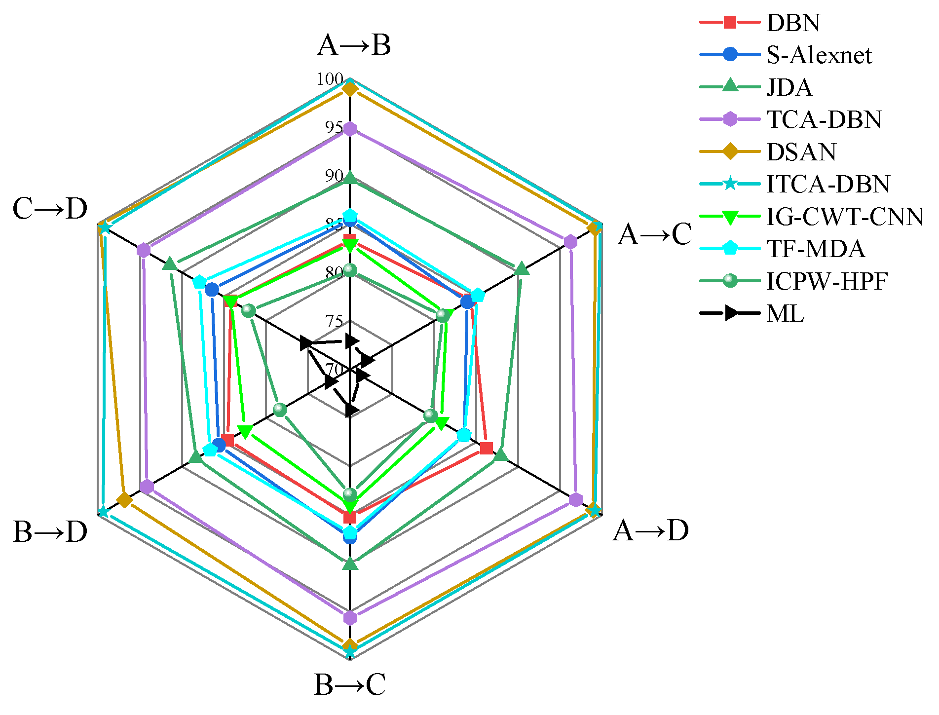
To verify the effectiveness of the proposed method, it was compared with the different methods: DBN, IG-CWT-CNN [31], TF-MDA [32], ICPW-HPF-CNN [33], ML [34], JDA [35], TCA-DBN [36], DSAN [18], and S-Alexnet [37]. The structure of the DBN was [80, 40, 40, 20], and the learning rate was 0.05. The structure of the DBN in the TCA-DBN model was [50, 30, 20], and the learning rate is 0.01. The structure of the DBN in the method proposed was [50, 30, 20], with a learning rate of 0.01, SRPLC-K-means preserves the top 80% of the samples. Based on multiple preliminary experiments, $u$ = 1/16 and $\lambda$ = 1/5 were ultimately selected. The fault diagnosis results of six cross-working condition tasks using the different methods are shown in

Table 3. Cross-working conditions fault diagnoses results using different methods.

Methods	A → B	A → C	A → D	B → C	B → D	C → D	Average Accuracy
DBN	83.333	84.375	86.25	85.208	84.583	84.167	84.653
S-Alexnet	85.417	83.958	83.542	87.292	85.625	86.458	85.382
IG-CWT-CNN	82.917	81.458	80.833	83.958	82.5	84.167	82.639
TF-MDA	85.833	85.208	83.542	86.875	86.667	87.927	86.009
ICPW-HPF	80.209	81.0417	79.583	82.917	78.333	82.083	80.694
ML	72.927	71.875	71.25	74.167	72.5	75.417	73.023
JDA	89.583	90.417	87.917	90.208	88.333	91.458	89.653
TCA-DBN	94.792	96.25	96.875	95.625	94.167	94.583	95.382
DSAN	98.958	99.167	98.958	98.542	96.875	99.792	98.715
ITCA-DBN	100	99.792	99.167	99.167	99.375	99.167	99.445

and Figure 6.

As shown in Table 3 and Figure 6, the average accuracy of DBN, S-Alexnet, IG-CWT-CNN, TF-MDA, ICPW-HPF-CNN, ML, JDA, TCA-DBN, DSAN, and ITCA-DBN were 84.653%, 85.382%, 82.639%, 86.009%, 80.649%, 73.023%, 85.382%, 89.653%, 98.582%, 98.715%, and 99.445%, respectively. Due to the DBN, IG-CWT-CNN, TF-MDA, ICPW-HPF-CNN, ML, and S-Alexnet, without considering the discrepancies in the data distribution under different working conditions, the fault diagnosis effect was poor. Due to JDA satisfying the equality of the joint probability density of the data distribution between the target domain and the source domain, it achieved a higher accuracy of 5%, 4.271%, 7.014%, 3.644%, 8.959%, and 16.63% compared to the DBN, S-Alexnet, IG-CWT-CNN, TF-MDA, ICPW-HPF-CNN, and ML respectively. However, JDA did not solve the problem of data distribution discrepancies in the subdomains, so its accuracy could only be maintained at approximately 90%. TCA-DBN globally aligned the data distribution between two domains but did not consider the discrepancies in the data distribution of the same fault type between different domains, resulting in an average accuracy of 95.382%. DSAN achieved subdomain adaptation using LMMD, with an average accuracy of 98.715%. The method proposed in this article aligns the data distribution discrepancies in the subdomains, resulting in an average accuracy of 99.445%. Although both the proposed method and DSAN use LMMD to achieve subdomain adaptation, the proposed method combines divergence factors and SRPLC-K-means, resulting in an accuracy of 0.73% higher than DSAN. Based on the fault diagnosis results of the different methods presented in Table 3 and Figure 6, it can be concluded that the proposed method outperforms the other different methods in diagnosing faults under cross-working conditions.

4.3. Test Ⅱ

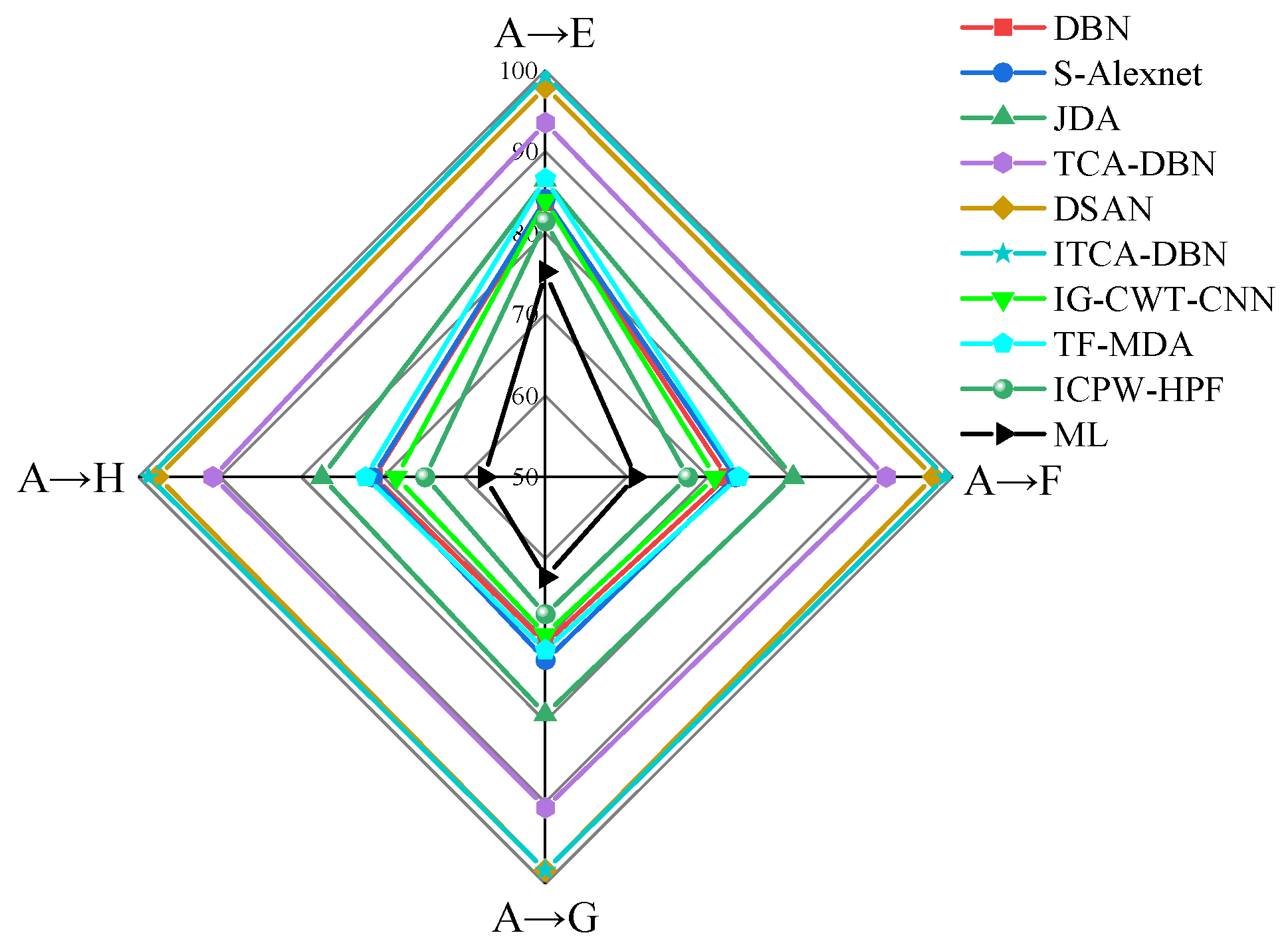
To verify the effectiveness of the proposed method for bearing fault diagnoses under different types and variable working conditions, the proposed method, DBN, S-Alexnet, IG-CWT-CNN, TF-MDA, ICPW-HPF-CNN, ML, JDA, TCA-DBN, and DSAN were used for cross types and cross-working condition fault diagnoses on datasets A, E, F, G, and H. There were four tasks of cross types and cross-working condition fault diagnoses, namely A → E, A → F, A → G, and A → H. The dataset allocation and parameter settings for each method in Test Ⅱ are the same as for Test Ⅰ. The fault diagnoses results are shown in

Table 4. Cross-type and cross-working condition fault diagnoses result from using different methods.

Methods	A → E	A → F	A → G	A → H	Average Accuracy
DBN	83.75	72.292	70.417	71.042	74.375
S-Alexnet	84.167	73.333	72.5	71.25	75.313
IG-CWT-CNN	83.958	70.833	69.375	68.333	73.125
TF-MDA	86.667	73.75	71.25	72.083	75.938
ICPW-HPF	81.458	67.5	66.875	64.792	70.156
ML	75.208	61.042	62.292	57.5	64.01
JDA	86.458	80.417	79.167	77.5	80.886
TCA-DBN	93.542	91.875	90.625	90.833	91.719
DSAN	97.917	97.708	98.333	97.708	97.916
ITCA-DBN	99.375	99.167	98.333	98.75	98.906

and Figure 7.

As shown in Table 4 and Figure 7, the average accuracy values of the DBN, S-Alexnet, IG-CWT-CNN, TF-MDA, ICPW-HPF-CNN, ML, JDA, TCA-DBN, DSAN, and ITCA-DBN were 74.375%, 75.313, 73.125%, 75.938%, 70.156%, 64.01%, 80.886%, 91.719%, 97.916%, and 98.906%, respectively. The JDA and TCA-DBN that achieve global domain adaptation can obtain better performance than the DBN, IG-CWT-CNN, TF-MDA, ICPW-HPF-CNN, ML, and S-Alexnet without using transfer learning. The accuracy of DSAN that achieves subdomain adaptation was higher than that of both JDA and TCA-DBN. The accuracy of the proposed method was 0.99% higher than that of DSAN. Due to changes in the bearing types and working conditions, the discrepancies in the data distribution between the source and target domains became more pronounced than just the changes in the working conditions, resulting in a decrease in the accuracy of all methods. Compared with the cross-working condition fault diagnosis test, the accuracy of the DBN, S-Alexnet, IG-CWT-CNN, TF-MDA, ICPW-HPF-CNN, ML, JDA, TCA-DBN, DSAN, and ITCA-DBN decreased by 10.278%, 10.069%, 9.541%, 10.072%, 10.538%, 9.013%, 8.767%, 3.663%, 0.799%, and 0.539%, respectively. The proposed method had the highest accuracy and the lowest reduction in accuracy, indicating the best performance. Based on the performance of ITCA-DBN, it can be seen that the proposed method can effectively achieve bearing fault diagnoses across types and cross-working conditions.

4.4. Feature Visualization

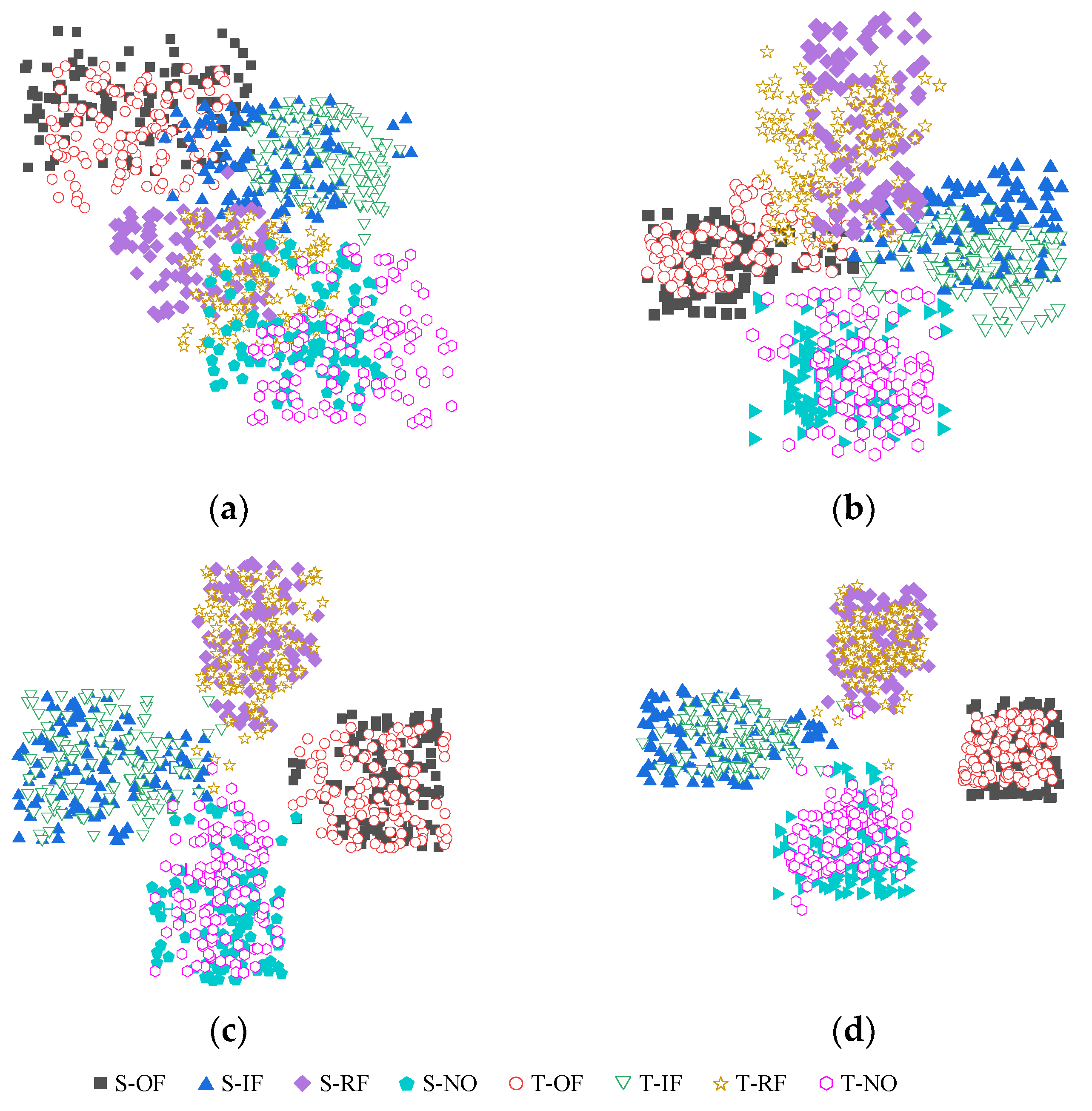
To further verify the fault classification effect of the proposed method in a bearing fault diagnosis, the t-distributed stochastic neighbor embedding [38] (t-SNE) was employed to reduce the dimensionality of the original data features, and the features were mapped using TCA, DSAN, and ITCA, respectively, taking the data of task A → F across the types and across working conditions as the object. The t-SNE could reduce the high-dimensional features into two-dimensional features, which were plotted using scatter plots to describe the classification ability of the different methods. The detailed visualization results are displayed in Figure 8. In Figure 8, S-OF, S-IF, S-RF, and S-NO represent the outer ring fault, inner ring fault, rolling element fault, and normal state in the source domain, respectively. T-OF, T-IF, T-RF, and T-NO represent the outer ring fault, inner ring fault, rolling element fault, and normal state in the target domain, respectively.

Figure 8a depicts the unprocessed original distribution of the sample features, and it can be observed that the four types of data in the source domain and the four types of data in the target domain were mixed and could not be distinguished. The distribution of the data within each individual domain, whether source or target, was highly distinguishable across the four categories. Figure 8b shows the feature distribution after TCA mapping. While the fault types in the figure are easier to distinguish, significant discrepancies persisted in the distribution of the same fault types between different domains, easily leading to confusion with other fault types. Figure 8c shows the feature distribution processed using DSAN. The distribution of the various types of data in the target domain was approximately aligned with the corresponding types of data in the source domain, resulting in a relatively clear decision boundary. Figure 8d shows the feature distribution after ITCA mapping, where various types of data in the target domain align with corresponding types of data in the source domain, featuring clear boundaries and easy distinction. From the results shown in Figure 8, we can notice that: (1) TCA that achieves domain adaptation can reduce the distribution discrepancies between different domains but the effect is inconspicuous. (2) DSAN that achieves subdomain adaptation can reduce the distribution discrepancies of the same fault types between different domains, rendering it easier to distinguish the fault types of the samples. However, there still were edge samples that were confused with other types. (3) ITCA, which combines domain adaptation and divergence factors, not only reduces the distribution discrepancies of the same fault types between different domains, but also increases the intraclass compactness of samples, decreases the edge samples, and enhances the sample distinguishability.

4.5. Test Ⅲ

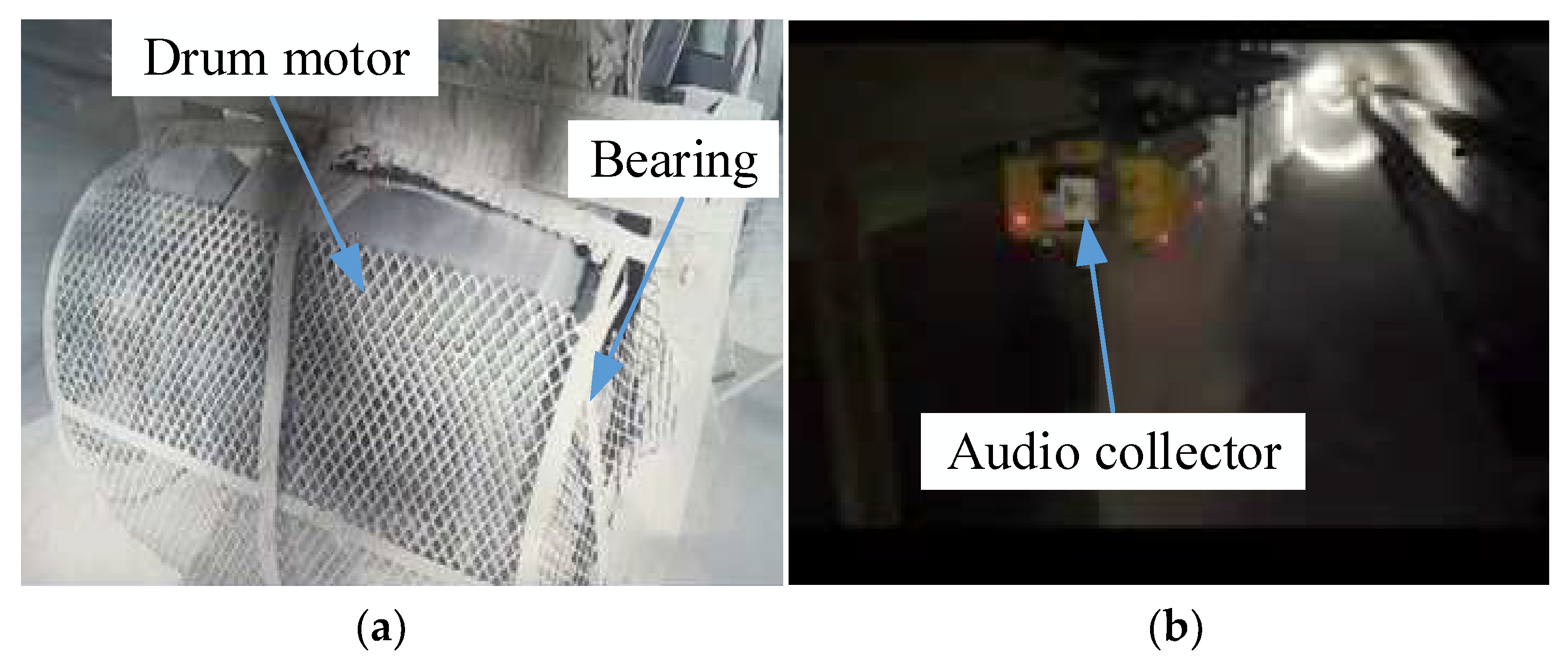
To further verify the cross-working conditions fault diagnosis ability of the proposed method, experimental verification was conducted on the bearing data of a drum motor for coal mine transportation collected underground in Xuzhou. The drum motor for coal mine transportation and audio collector are shown in Figure 9. The data used in test Ⅲ were underground audio signals. There were four health statuses, namely bearing outer ring damage, rolling element damage, inner ring damage, and the normal state. We collected data under the working conditions of 500 r/min, 750 r/min, and 1000 r/min. The specific information of the bearing dataset for the drum motor is shown in

Table 5. Dataset of the drum motor bearings.

Working Conditions	Rotational Speeds	Health Status
I	500 r/min	Normal state Inner ring fault Rolling element fault Outer ring fault
J	750 r/min
K	1000 r/min

.

There were three cross-working condition fault diagnosis tasks in test Ⅲ, namely I → J, I → K, and J → K. We compared the different methods of DBN, S-Alexnet, IG-CWT-CNN, TF-MDA, ICPW-HPF-CNN, ML, JDA, TCA-DBN, and DSAN with the proposed method. The detailed fault diagnosis results are presented in

Table 6. Diagnosis results of the bearing faults in the drum motor.

Methods	I → J	I → K	J → K	Average Accuracy
DBN	68.125	66.25	71.042	68.472
S-Alexnet	70.625	66.042	67.083	67.917
IG-CWT-CNN	67.292	66.875	65.417	66.528
TF-MDA	71.042	72.083	69.167	70.764
ICPW-HPF	64.792	63.75	62.292	63.611
ML	55.625	53.75	54.375	54.583
JDA	71.25	67.083	70.625	69.653
TCA-DBN	82.083	78.958	80.625	80.555
DSAN	86.875	84.167	88.125	86.389
ITCA-DBN	92.083	90.833	92.917	91.944

and Figure 10.

As shown in Table 6 and Figure 10, the average accuracy of the DBN, S-Alexnet, IG-CWT-CNN, TF-MDA, ICPW-HPF-CNN, ML, JDA, TCA-DBN, DSAN, and ITCA-DBN were 68.472%, 67.917%, 66.528%, 70.764%, 63.611%, 54.583%, 69.653%, 80.555%, 86.389%, and 91.944%, respectively. Due to the low signal-to-noise ratio of the data in this experiment, the accuracy of the cross-working condition fault diagnosis was lower than that of test Ⅰ. The average accuracy of ITCA-DBN was the highest, and the effect was better than that of the other methods. Compared to TCA-DBN and DSAN, the average accuracy of ITCA-DBN increased by 11.389% and 5.555%, respectively. Based on the above comparative analysis, it can be clearly seen that the proposed ITCA and SRPLC K-means contributed to diagnosing faults under variable working conditions.

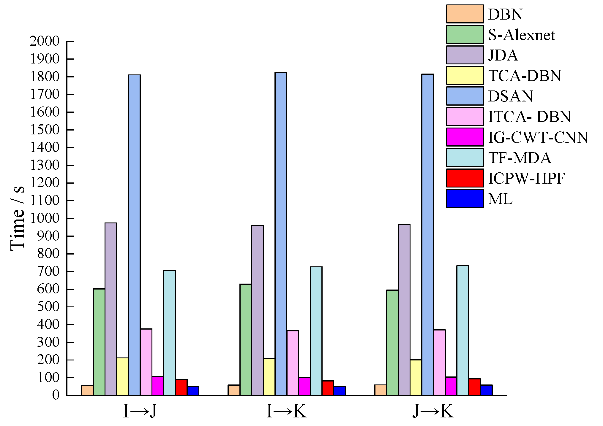
To demonstrate that the fault diagnosis using the proposed method required less time, the time required for different methods to achieve fault diagnosis was calculated. The time required for different different methods is presented in

Table 7. The time (s) consumed using each method for the fault diagnosis.

Methods	I → J	I → K	J → K	Average Time
DBN	54.3	58.7	59.6	57.5
S-Alexnet	601.6	628.4	594.5	608.7
IG-CWT-CNN	106.7	99.6	103.4	103.2
TF-MDA	706.6	726.5	733.8	722.3
ICPW-HPF	89.8	81.5	93.4	88.2
ML	50.9	51.3	58.8	53.7
JDA	974.5	961.2	965.2	967
TCA-DBN	212.3	209.7	200.7	207.6
DSAN	1811.2	1825.4	1814.3	1817
ITCA-DBN	375.6	364.9	370.7	370.4

and Figure 11. We started timing from processing the raw data and stopped timing when we obtained the output diagnostic results for the test set.

As shown in Table 7 and Figure 11, the average time required for DBN, S-Alexnet, IG-CWT-CNN, TF-MDA, ICPW-HPF-CNN, ML, JDA, TCA-DBN, DSAN, and ITCA-DBN to complete three cross-working condition fault diagnosis tasks was 57.5 s, 608.7 s, 103.2 s, 722.3 s, 88.2 s, 53.7 s, 960.3 s, 207.6 s, 1797 s, and 365.4 s, respectively. Due to the simple structure and low computational complexity of DBN, IG-CWT-CNN, ICPW-HPF-CNN, and ML, these models require less time to complete fault diagnoses. S-Alexnet uses lightweight convolutional neural networks to extract features, which requires more time to complete a fault diagnosis. TF-MDA employs a one-dimensional convolutional neural network that integrates an attention mechanism to extract features, resulting in a longer time required for a fault diagnosis. JDA and DSAN require a large-scale convolutional neural network to extract raw signal features, resulting in significantly longer required time. Compared to TCA-DBN, the objective function of ITCA-DBN is more complex and has additional marking pseudo labels and SRPLC K-means steps, thus requiring more time. Combining Table 6 and Table 7, compared with DBN and TCA-DBN, although ITCA-DBN takes longer than DBN and TCA-DBN, its accuracy is higher. Compared with S-Alexnet, DSAN, and JDA, ITCA-DBN not only requires less time but also has higher accuracy. Compared with the other different methods, the proposed method has the optimal performance for fault diagnoses.

5. Conclusions

To reduce the time required for cross-working condition fault diagnoses and improve the accuracy, we improved TCA, filtered out the noisy samples and corrected pseudo labels. This paper proposed a novel bearing fault diagnosis method named the improved transfer component analysis and deep belief network. The ITCA uses LMMD instead of MMD, achieving subdomain adaptation and adding the divergence factor into the objective function to increase intraclass compactness. Additionally, to improve the accuracy of the pseudo labels in the validation set, SRPLC-K-means was designed to filter the noisy samples and correct the pseudo labels, resulting in higher confident pseudo labels. Based on two tests using the CWRU bearing dataset and a test using underground drum motor bearing data, the following conclusions are drawn:

(1) ITCA can significantly reduce the distribution discrepancies of the same type of data between different domains, achieve subdomain adaptation, and improve the intraclass compactness of the samples. According to the results of the three tests, the proposed method achieves diagnostic accuracies of 99.445%, 98.906%, and 91.944%, respectively, surpassing other methods;

(2) The proposed SRPLC-K-means contributed to diagnosing faults under variable working conditions;

(3) Compared to end-to-end models, such as JDA and DSAN, the proposed method reduced the required time by 594.9 s and 1431.6 s, respectively, while increasing the accuracy by 22.291% and 5.555%, respectively.

We should note that the proposed method is currently only applicable to datasets with balanced numbers of each fault type and from a single source domain. In the future, we plan to explore subdomain adaptations, clustering domain adaptation, and noise reduction algorithms to cater to more demanding industrial requirements.

References

1. Yin, C.; Wang, Y.; Ma, G.; Wang, Y.; Sun, Y.; He, Y. Weak fault feature extraction of rolling bearings based on improved ensemble noise-reconstructed EMD and adaptive threshold denoising. Mech. Syst. Signal Process. 2022, 171, 108834. [Google Scholar] [CrossRef]
2. Liu, Q.; Chen, F.; Zhou, Z.; Wei, Q. Fault diagnosis of rolling bearing based on wavelet package transform and ensemble empirical mode decomposition. Adv. Mech. Eng. 2019, 5 Pt 2, 792584. [Google Scholar] [CrossRef]
3. Liang, P.; Wang, W.; Yuan, X.; Liu, S.; Zhang, L.; Cheng, Y. Intelligent fault diagnosis of rolling bearing based on wavelet transform and improved ResNet under noisy labels and environment. Eng. Appl. Artif. Intell. 2022, 115, 105269. [Google Scholar] [CrossRef]
4. Lei, C.; Xia, B.; Xue, L. Rolling bearing fault diagnosis method based on MTF-CNN. J. Vib. Shock 2022, 41, 151–158. [Google Scholar]
5. Xu, X.; Cao, D.; Zhou, Y. Application of neural network algorithm in fault diagnosis of mechanical intelligence. Mech. Syst. Signal Process. 2020, 141, 106625. [Google Scholar] [CrossRef]
6. Umang, P.; Pandya, D. Experimental investigation of cylindrical bearing fault diagnosis with SVM. J. Vib. Shock 2021, 44, 1286–1290. [Google Scholar]
7. Mohammad, H.; Mahmoud, O.; Ebrahim, B. Fault diagnosis of tractor auxiliary gearbox using vibration analysis and random forest classifier. Inf. Process. Agric. 2022, 9, 60–67. [Google Scholar]
8. Gong, M.; Guo, Y.; Yan, P.; Wu, N.; Zhang, C. A new fault diagnosis method of rolling bearings of shearer. Ind. Mine Autom. 2017, 43, 50–53. [Google Scholar]
9. Lei, X.; Lu, N.; Chen, C. An AVMD-DBN-ELM model for bearing fault diagnosis. Sensors 2022, 22, 9369. [Google Scholar] [CrossRef]
10. Zhang, J.; Ren, C. Rolling bearing feature transfer diagnosis based on deep belief network. J. Vib. Meas. Diagn. 2022, 42, 277–284+407. [Google Scholar]
11. Ye, N.; Chang, P.; Zhang, L.; Wang, J. Research on multi-condition bearing fault diagnosis based on improved semi-supervised deep belief network. J. Mech. Eng. 2021, 57, 80–90. [Google Scholar]
12. Wang, C.; Chen, D.; Chen, J.; Lai, X.; He, T. Deep regression adaptation networks with model-based transfer learning for dynamic load identification in the frequency domain. Eng. Appl. Artif. Intell. 2021, 102, 104244. [Google Scholar] [CrossRef]
13. Pang, B.; Liu, Q.; Sun, Z.; Xu, Z.; Hao, Z. Time-frequency supervised contrastive learning via pseudo-labeling: An unsupervised domain adaptation network for rolling bearing fault diagnosis under time-varying speeds. Adv. Eng. Inform. 2024, 59, 102304. [Google Scholar] [CrossRef]
14. Li, X.; Hu, Y.; Zheng, J.; Li, M.; Ma, W. Central moment discrepancy based domain adaptation for intelligent bearing fault diagnosis. Neurocomputing 2021, 429, 12–24. [Google Scholar] [CrossRef]
15. Ma, W.; Zhang, Y.; Ma, L. Sliced An unsupervised domain adaptation approach with enhanced transferability and discriminability for bearing fault diagnosis under few-shot samples. Expert Syst. Appl. 2023, 225, 120084. [Google Scholar] [CrossRef]
16. Kmjad, Z.; Sikora, A. Bearing fault diagnosis with intermediate domain based Layered Maximum Mean Discrepancy: A new transfer learning approach. Eng. Appl. Artif. Intell. 2021, 105, 104415. [Google Scholar]
17. Chen, C.; Fu, Z.; Chen, Z.; Jin, S.; Cheng, Z.; Jin, X.; Hua, X.-S. HoMM: Higher-order moment matching for unsupervised domain adaptation. Proc. AAAI Conf. Artif. Intell. 2020, 34, 3422–3429. [Google Scholar] [CrossRef]
18. Zhu, Y.; Zhuang, F.; Wang, J.; Ke, G.; Chen, J.; Bian, J.; Xiong, H.; He, Q. Deep subdomain adaptation network for image classification. IEEE Trans. Neural Netw. Learn. Syst. 2020, 32, 1713–1722. [Google Scholar] [CrossRef] [PubMed]
19. Wang, P.; Yang, G.; Li, Y.; Li, P.; Guo, Y.; Chen, R. Deep sample clustering domain adaptation for breast histopathology image classification. Biomed. Signal Process. Control 2024, 87, 105500. [Google Scholar] [CrossRef]
20. Tian, M.; Su, X.; Chen, C.; An, W.; Sun, X. Research on domain adaptive fault diagnosis method for wind turbine generator bearings. Acta Energiae Solaris Sin. 2023, 44, 310–317. [Google Scholar]
21. Chen, P.; Zhao, R.; He, T.; Wei, K.; Yang, Q. Unsupervised domain adaptation of bearing fault diagnosis based on Join Sliced Wasserstein Distance. ISA Trans. 2022, 129, 504–519. [Google Scholar] [CrossRef]
22. Liu, Y.; Wang, Y.; Chow, T.W.S.; Li, B. Deep adversarial subdomain adaptation network for intelligent fault diagnosis. IEEE Trans. Ind. Inform. 2022, 18, 6038–6046. [Google Scholar] [CrossRef]
23. Kouw, W.M.; Loog, M. A review of single-source unsupervised domain adaptation. arXiv 2019, arXiv:1901.05335. [Google Scholar]
24. Pan, S.J.; Tsang, I.W.; Kwok, J.T.; Yang, Q. Domain adaptation via transfer component analysis. IEEE Trans. Neural Netw. 2011, 22, 199–210. [Google Scholar] [CrossRef] [PubMed]
25. Su, Y.; Huang, H.; Lai, X.; Chen, Y.; Yang, L.; Lin, C.; Xie, X.; Huang, B. Evaluation of landslide susceptibility of reservoir bank trans-regional Based on transfer component analysis. Earth Sci. 2023, 1–21. [Google Scholar] [CrossRef]
26. Sujatha, K.; Yu, W.; Jin, L.; Seifedine, K. GO-DBN: Gannet optimized deep belief network based wavelet kernel elm for detection of diabetic retinopathy. Expert Syst. Appl. 2023, 229, 120408. [Google Scholar]
27. Wang, G.; Qiao, J.; Bi, J.; Li, W.; Zhou, M. TL-GDBN: Growing deep belief network with transfer learning. IEEE Trans. Autom. Sci. Eng. 2019, 16, 874–885. [Google Scholar] [CrossRef]
28. Sharma, A.; Kalluri, T.; Chandraker, M. Instance level affinity-based transfer for unsupervised domain adaptation. In Proceedings of the IEEE/CVF Conference on Computer Vision and Pattern Recognition, Nashville, TN, USA, 20–25 June 2021; pp. 5361–5371. [Google Scholar]
29. Smith, W.A.; Randall, R.B. Rolling element bearing diagnostics using the Case Western Reserve University data: A benchmark study. Mech. Syst. Signal Process. 2015, 64–65, 100–113. [Google Scholar] [CrossRef]
30. Jiao, J.; Yue, J.; Pei, D. Rolling bearing fault diagnosis method based on MSK-SVM. J. Electron. Meas. Instrum. 2022, 36, 109–117. [Google Scholar]
31. Du, J.; Li, X.; Gao, Y.; Gao, L. Integrated Gradient-Based Continuous Wavelet Transform for Bearing Fault Diagnosis. Sensors 2022, 22, 8760. [Google Scholar] [CrossRef]
32. Kim, Y.; Kim, Y. Time-Frequency Multi-Domain 1D Convolutional Neural Network with Channel-Spatial Attention for Noise-Robust Bearing Fault Diagnosis. Sensors 2023, 23, 9311. [Google Scholar] [CrossRef] [PubMed]
33. Kiakojouri, A.; Lu, Z.; Mirring, P.; Powrie, H.; Wang, L. A Novel Hybrid Technique Combining Improved Cepstrum Pre-Whitening and High-Pass Filtering for Effective Bearing Fault Diagnosis Using Vibration Data. Sensors 2023, 23, 9048. [Google Scholar] [CrossRef] [PubMed]
34. Bertocco, M.; Fort, A.; Landi, E.; Mugnaini, M.; Parri, L.; Peruzzi, G.; Pozzebon, A. Roller Bearing Failures Classification with Low Computational Cost Embedded Machine Learning. In Proceedings of the 2022 IEEE International Workshop on Metrology for Automotive (MetroAutomotive), Modena, Italy, 4–6 July 2022; pp. 12–17. [Google Scholar]
35. Han, T.; Liu, C.; Yang, W.; Jiang, D. Deep transfer network with joint distribution adaptation: A new intelligent fault diagnosis framework for industry application. ISA Trans. 2020, 97, 269–281. [Google Scholar] [CrossRef] [PubMed]
36. Duan, L.; Xie, J.; Wang, K.; Wang, J. Gearbox diagnosis based on auxiliary monitoring datasets of different working conditions. J. Vib. Shock 2017, 36, 104–108+116. [Google Scholar]
37. Ding, X.; Wang, H.; Cao, Z.; Liu, X.; Liu, Y.; Huang, Z. An Edge Intelligent Method for Bearing Fault Diagnosis Based on a Parameter Transplantation Convolutional Neural Network. Electronics 2023, 12, 1816. [Google Scholar] [CrossRef]
38. Bibal, A.; Delchevalerie, V.; Frénay, B. DT-SNE: T-SNE discrete visualizations as decision tree structures. Neurocomputing 2023, 529, 101–112. [Google Scholar] [CrossRef]
Figure 1. Global domain adaptation and subdomain adaptation.
Applsci 14 01973 g001
Figure 2. Structure of a DBN.
Applsci 14 01973 g002
Figure 3. The flowchart of the SRPLC-K-means method.
Applsci 14 01973 g003
Figure 4. Illustration of the SRPLC-K-means methods.
Applsci 14 01973 g004
Figure 5. The fault diagnosis flow chart of the proposed method.
Applsci 14 01973 g005
Figure 6. Radar chart of cross-working conditions fault diagnoses results using different methods.
Applsci 14 01973 g006
Figure 7. Radar chart of cross types and cross-working conditions fault diagnoses results using different methods.
Applsci 14 01973 g007
Figure 8. Feature visualization results. (a) Original distribution of the sample features; (b) TCA; (c) DSAN; (d) ITCA.
Applsci 14 01973 g008
Figure 9. Drum motor for the coal mine transportation (the collected data on the bearings of the underground drum motor was used for the cross-working condition fault diagnosis). (a) Drum motor; (b) Audio acquisition device.
Applsci 14 01973 g009
Figure 10. Radar chart of the bearing fault diagnosis results in the drum motor.
Applsci 14 01973 g010
Figure 11. Bar chart of the time consumed using each method for the fault diagnosis.
Applsci 14 01973 g011