Abstract
Fluid migration in a fracture network plays an important role in the oil accumulation mechanism and hence is key to oil exploration. In this study, we build a model by combining one-dimensional (1D) Navier–Stokes equations, linear elastic equations, and energy equations, and validate the model by reproducing the thickness profile of a fluid-driven crack measured in an experiment. We employ this model to simulate the upward flow of viscous fluid in a single fracture during hydrocarbon migration. The simulation suggests that the parameters of both the fluid and the surrounding rock matrix, as well as the boundary condition imposed on the fracture outlet, affect the upward flow in the fracture. We then extend our model from the single fracture to the bifurcated fracture and the fracture network by maintaining homogeneous pressure and mass conservation at the connection of the channels. We find that the increase in network complexity leads to an increase in the inlet pressure gradient and inlet speed, and a decrease in the outlet pressure gradient and outlet speed. The effective area where the fluid is driven upward from the inlet to the outlet is offset toward the inlet. More importantly, the main novelty of our model is that it allows us to evaluate the effect of inconsistencies in individual branch parameters, such as matrix stiffness, permeability, temperature, and boundary conditions, on the overall upward flow of viscous fluid. Our results suggest that the heterogeneity enforces the greater impact on the closer branches.
1. Introduction
In the past decade, oil production from unconventional subsurface resources such as ultra-tight organic-rich shale has increased significantly [1]. According to data released by the IEA, unconventional oil will account for more than 30% of total oil production by 2030 [2]. In unconventional oil production, the stored oil flows through the natural and hydraulic fractures formed in the rock matrix to reach the production wells [3]. Therefore, understanding the physical process of oil migration in fractures is a critical objective. However, because the mechanical behavior of a fractured rock matrix shows obvious heterogeneity and anisotropy [4,5], it is difficult to scale the structure of the fractured rock matrix that the oil migrates through. Moreover, the complexity of the fracture network is a huge challenge for predicting the interaction between the liquid flow and the surrounding rock.
Depending on their geological origin, natural fractures can consist of structural fractures formed under tectonic stress, non-structural fractures caused by factors such as dehydration and weathering, and organic-matter-related fractures formed due to abnormal hydrocarbon generation and the thermal evolution of organic matter [6]. Gong et al. identified 2235 fractures in shale core samples, of which structural fractures accounted for 77.5% [7]. Ogata et al. analyzed the fractures and faults of the Jurassic Entrada Formation in the northernmost part of Paradox Basin located at the northwestern edge of the Colorado Plateau in central Utah. And identified structural fracture corridors propagating in an approximately vertical direction from the bottom to the top [8], as shown in Figure 1a. Wang et al. further demonstrated the vertical propagating behavior of a structural fracture based on the characteristics of the Kongdong fault section in the Wangguantun area [9]. Using seismograms, Cartwright et al. predicted that structural fractures may also be the main fracture type in sedimentary basins [10,11]. As shown in Figure 1b, structural fractures disrupt the sealing sequence of a rock matrix and allow vertical or sub-vertical fluid migration in the rock matrix.
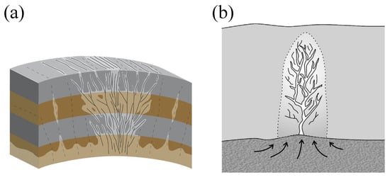
Figure 1.
(a) A conceptual cartoon proposed by Ogata et al. showing a fold-related crestal fracture corridor with a network of fluid flow pathways [8]. (b) The conceptual model proposed by Cartwright et al., for fluid escape path growth by hydraulic fracturing in a sedimentary basin [11].
In recent years, three main types of numerical models have been developed to describe the hydrocarbon migration process in a fracture network: equivalent continuum models, discrete fracture models, and hybrid models. The equivalent continuum model (ECM) employs the continuum method to capture the rock mass seepage based on the permeability coefficient tensor, assuming that the fractures have a sufficient number of random occurrences and are connected to each other [12]. Chaudhary et al. [13] and Agboada et al. [14] simulated a fracture network using logarithmic mesh encryption technology combined with the double porosity model to describe the changes of pressure and saturation near the fracture better. Therefore, the flow pattern in the complex fracture network of a shale oil reservoir can be characterized more accurately. The discrete fracture model (DFM) determines the evolution of the migrating fluid in each fracture by solving the mass conservation equation associated with the suitable boundary condition [15]. Jiang and Younis [16] established an embedded discrete fracture model (EDFM) to capture the interaction between the fluid and the surrounding rock matrix efficiently. Both the DFM and EDFM require a clear understanding of the spatial distribution of each fracture. They have higher accuracy than the ECM and can accurately describe the occurrence and distribution of fractures. However, their complexity leads to long simulation times and meshing difficulties in poor-quality meshing.
The hybrid model is a combination of the ECM and DFM and is the latest technology. It can simulate continuously distributed micro-fractures in the ECM part while capturing explicit fractures using the DFM. It is expected to satisfy calculation accuracy requirements while saving computing resources [17]. For example, Liu et al. [18] used a hybrid model to study the leakage of natural fractures, focusing on their theoretical leakage characteristics. Xu et al. [19] established a grid model for hydraulic fracturing simulation, in which there are two groups of mutually perpendicular plane fractures in the ellipse of the simulation region. Weng et al. [20] proposed a new fracture model to simulate complex fracture network expansion in naturally fractured formations. The interaction, coupling, and deformation of hydraulic fractures and natural fractures are considered in the model. Geng et al. [21] established a discrete fracture network based on the normal distribution of fracture length, and further developed a gas production prediction model for fractured shale reservoirs. When evaluating the reservoir performance of shale oil reservoirs, Zhang et al. [22] found that the fractal discrete fracture network model well characterized the fracture characteristics. Such studies have shed light on the effect of parameters such as rock permeability, fluid viscosity, and fluid pressure on the migration process. However, the interactions between the migration process and the shape of the fracture network are rarely straightforward to interpret.
The goal of this paper is to develop a comprehensive model to simulate fluid migration in a structural fracture network with heterogeneous properties by fully considering the role of a rock matrix on the flow dynamics in the fracture, as well as the feedback of the fluid flow to the shape of the fractures. This model simplifies the pressure-driven upflow in each fracture to a fully developed laminar flow between two infinite plates, and hence employs 1D Navier–Stokes equations to describe the mass and momentum conservation of the fluid flow in the vertical direction. In the lateral direction, we assume the surrounding rock matrix to be a set of spring matrices and achieve a balance between the pressure of the fluid and the elastic force of the rock matrix using the linear deformation law proposed by Ozdemirtas et al. [23]. This balance is dynamic, and hence the larger the pressure is, the larger is the corresponding fracture aperture.
In this work, we validate our model by reproducing a thickness profile of a fluid-driven crack, which is measured in the experiment [24], and then apply the model to describe the effects of various physical parameters of rock matrix and liquid as well, as structural fracture heterogeneity, on the steady-state migration that is reached with an equilibrium between liquid loss through the rock matrix and continuous replenishment from the source rock [25]. We first study the role of the thermal and dynamic parameters of the fluid and the rock matrix in the upflow in a single fracture using the model. Imposing suitable boundary conditions, we apply either an “open” or “closed” status to the outlet of the fracture in order to simulate the upflow in both the sealed fracture and the fracture connecting the reservoirs or the “sweet spots” [9]. At the same time, the study of the transition from open state to closed state is helpful in providing theoretical guidance for the new technology of oil exploitation—temporary-plugging-and-diverting fracturing (TPD fracturing). TPD fracturing technology is widely used in the re-fracturing of low production wells and completed wells. It can increase production by artificially sealing existing fractures and creating new fracture pathways in the formation [26,27,28]. We then apply our model to a bifurcated fracture that includes three connected channels to evaluate the effect of heterogeneous properties and the boundary conditions of the channels on the upflow within the whole fracture. Finally, we extend our model to a fracture network consisting of n levels of fractures. In contrast to previous studies [29], which assumed the homogeneous channels to be on the same level, our model allows heterogeneous flow in each channel, providing an opportunity for us to analyze deeply how the parameters changing in a channel can alter the flow fields of other channels on the same level.
2. The Upward Flow of a Viscous Liquid in a Single Fracture
We first investigate the flow dynamics coupled with the thermal process in a single fracture using a model involving suitable governing equations and boundary conditions.
2.1. Model
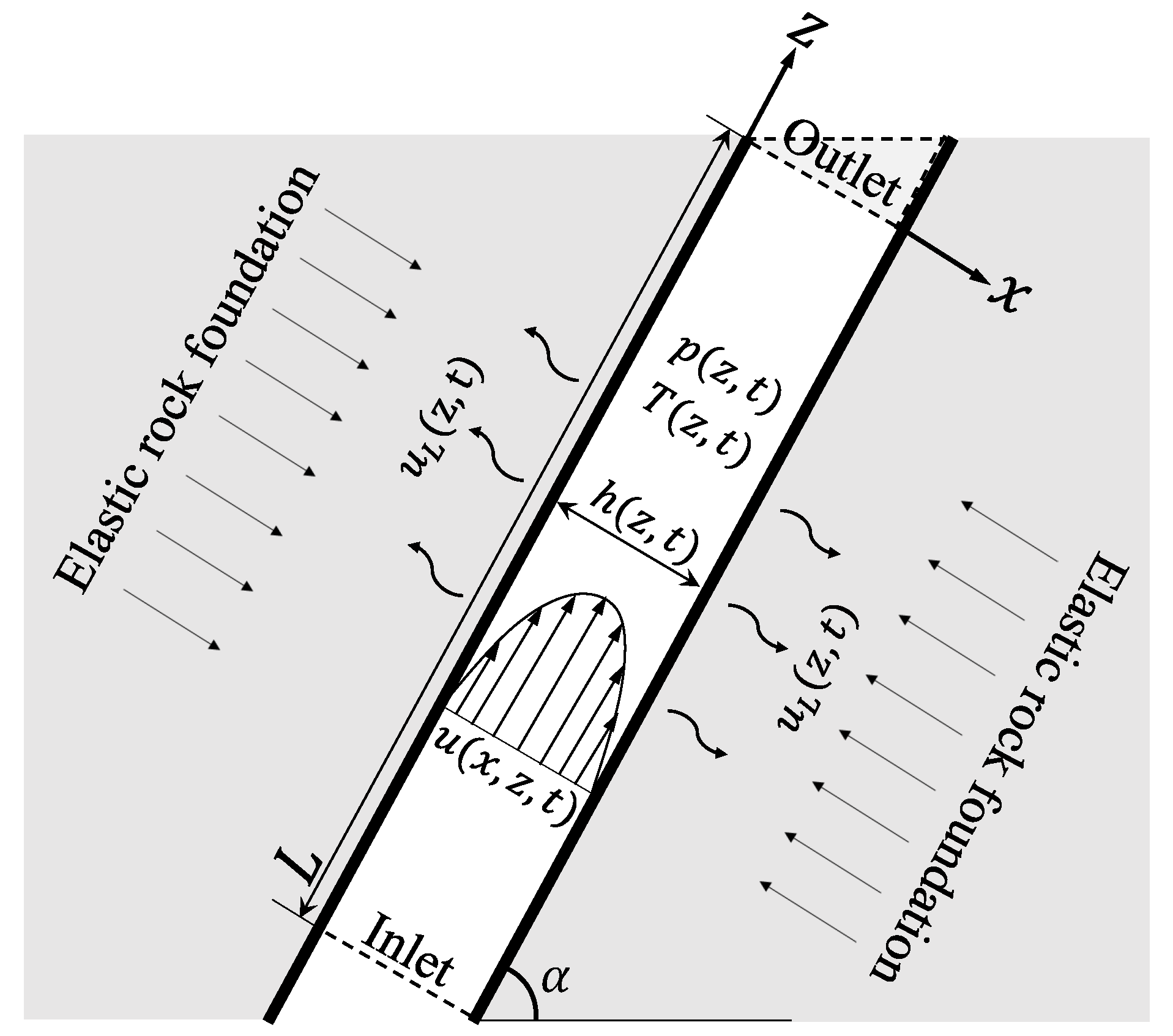
Figure 2 illustrates our model for the liquid flow in a single fracture with a length of L and an inclination angle of .
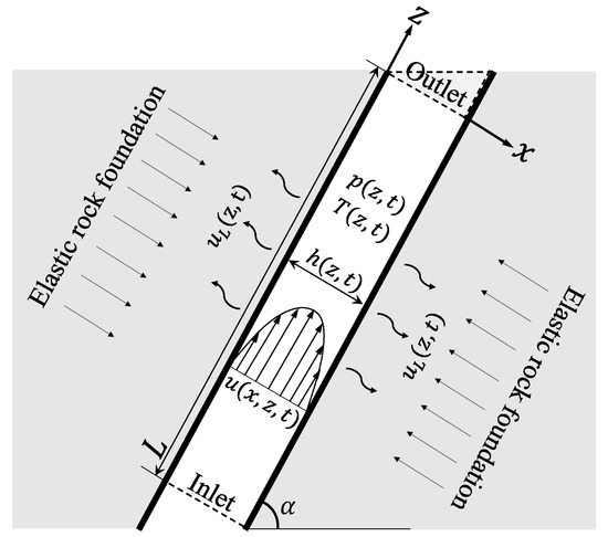
Figure 2.
Model of a single fracture. For an opened fracture, the triangle surrounded by the dashed line is removed, while the triangle seals the outlet for a closed fracture.
2.1.1. Governing Equations
We describe the steady-state Newtonian flow in a single fracture of inclination from the horizontal coordinate using the following 1D Navier–Stokes equations along the horizontal coordinate,
where u represents the vertical speed, is the dynamic viscosity, p is the pressure, is the density, g is the gravitational acceleration, and h is the aperture of the fracture. In this study, we neglect the gravitational term because it is approximately three orders of magnitude lower than the pressure term. The boundary conditions on the two walls are no-slip, as follows,
Integrating Equation (1), while accounting for the boundary condition of Equation (2), we obtain the relationship between the mean vertical speed, , and the pressure gradient, , as follows,
Our model is concerned with laminar flow between two infinite plates. Therefore, the following relationship should be satisfied,
where Re represents the Reynolds number.
Considering the impact of matrix leakage on the fracture walls [30], we apply the mass conservation law to a short length, , in the vertical coordinate to obtain
where represents the leakage velocity from the natural fracture to the rock matrix. Based on Darcy’s law, the leakage rate is proportional to the pressure difference in the x direction across the fracture wall and can be computed as
where is the ratio of the permeability of the rock foundation to the rock thickness, and represents the back pressure. Simplifying Equation (5) gives a one-dimensional continuity equation as
We assume the density of the liquid is constant because of the very low compressibility, but consider the variation of the viscosity along the vertical coordinate. Therefore, Equation (7) transforms into
Substituting Equation (3) into Equation (8), we obtain the following nonlinear equation for the evolution of the aperture,
In this study, we use the relationship given by Guo and Liu [30] to describe the variation of the viscosity caused by the temperature,
where represents the reference viscosity module and the temperature thinning module, defined as
where represents the Arrhenius activation energy required to induce thermal thinning, R is the universal gas constant, T is the temperature of the fluid, and is the reference temperature.
The temperature distribution of fractures during oil migration has been studied [31,32,33]. In this paper, the temperature of natural cracks is described by the method proposed by Whitsitt [34]. Our proposed model includes leakage from fractures to the rock matrix, so our temperature model should also include leakage effects. The temperature equation is described as follows:
where represents the temperature at the inlet of the fracture and is the temperature of the rock matrix. The is the coefficient of the energy equation. The length scale, , relates to the length of the leaked feature. The description is as follows:
where is the velocity at the fracture inlet that can be computed using Equation (3), and represents the inlet aperture of the fracture. The coefficient in Equation (12) is defined as
where is the reservoir porosity, and we compute as
where represents the error function. The parameter in Equations (14) and (15) depends on the physical parameters of the liquid as
where and C are the density and specific heat of the liquid, and , , and are the density, specific heat, and thermal conductivity of the rock matrix, respectively.
Considering that rock is an elastic material, in this study we assume the fracture is formed by the intrusion of high-pressure flow [23], and thereby employ the PKN model [35] to build the following correlation on the basis of the balance between the elastic force of the rock foundation and the pressure of the high-pressure flow,
where represents the original fracture aperture caused by the original pressure, , and is the fracture stiffness. It should be noted that the accuracy of the linear correlation in Equation (16) depends on the range of pressure changes during expansion and the initial value of pressure [23]. In this study, we set the initial pressure, , to be identical to the back pressure, .
2.1.2. The Numerical Scheme, Boundary and Initial Conditions, and Parameters
To capture the evolution of the fracture aperture and the flow dynamics, we build the governing equation by combining Equation (17) with Equation (9). We then employ an implicit time-stepping scheme and the standard second-order central difference method to discretize the governing equation. More details of our numerical scheme are presented in Appendix A.
In all computations in this study, we impose a constant pressure, , at the inlet of the fracture as
At the outlet of the fracture, however, we define two types of boundary conditions, as illustrated in Figure 2. The first one is an “open” outlet, for which we impose a constant outlet pressure as
For the computation shown in the results section, we set the outlet pressure, , to be equal to the original pressure, . The second option is to assume a “closed” outlet. We impose a constant speed, , at the “closed” outlet in order to allow the outlet of fracture to propagate. Hence, the gradient of the pressure at the outlet is
where and are, respectively, the liquid viscosity and fracture aperture at the outlet.
In the simulation with either an open or closed outlet, we define the initial pressure to vary linearly from to .
2.2. The Validation of Our Model
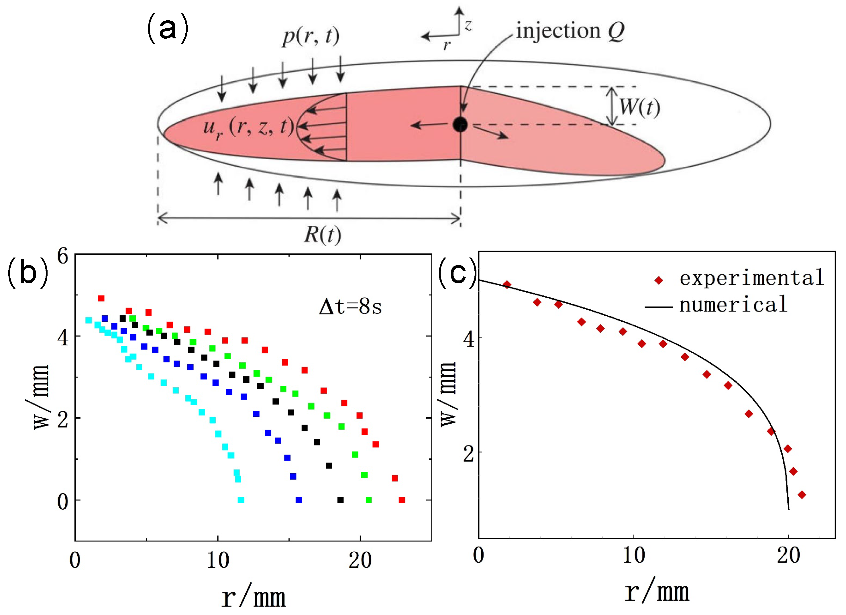
To validate our model, we reproduced a thickness profile of a fluid-driven crack, which was measured in the experiment by Lai et al. [24]. As illustrated in Figure 3a, the fluid was injected into the elastic matrix (gelatin) through a syringe pump, then forming a penny-shaped crack. Driven by the pressure, the crack grew, gradually expanding in the radial (y-) and thick (z-) directions. The geometrical size in the thick direction, 2 W, represents the thickness of the crack, which reduces from the injection point (where r = 0) to the rim of the crack (where r = R). Figure 3b is the thickness distribution we reproduced in the article. The light blue line shows the thickness distribution data for the first crack (28 s). The data were then recorded every 8 s until the liquid in the injection pump was fully injected into the gelatin matrix (60 s) and maintained at this state. We assumed that the fracture was fully developed in 60 s. In the experiment, the elastic modulus of the matrix, E, was 202 kPa, and the viscosity of the fluid was 1.02 Pa s.
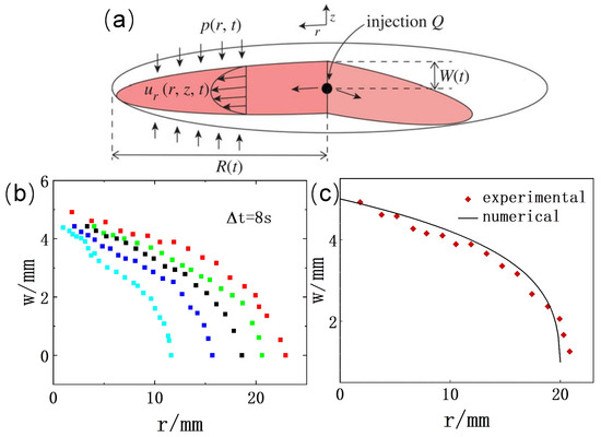
Figure 3.
(a) Schematic diagram of a penny-shaped crack, proposed by Lai et al. [24]. (b) Reproduced w (thickness)-r (length) distribution map. (c) The comparison between our numerical reproduction (NUM) and the experimental measurement (EXP) of the crack thickness, h = W, on r = 0 to 20 mm at the time of 60 s.
We read the thickness distribution for r = 0 to 20 mm at the time of 60 s (red line) from Figure 3b, and compare its to the numerical reproduction of our model. In the calculation, we use the experimental size parameters to calculate. Since the thickness of the crack is measured in millimeters, we set the stiffness of the matrix to 2.02 × 10⁸ Pa/m and the value of L to 20 mm. Due to the small experimental size, the viscosity of the liquid is assumed to remain unchanged at 1.02 Pa s. The temperature of the rock matrix remains unchanged at 25 °C. The pressure at the boundary is obtained from the measured crack thickness at r = 0 and r = 20 mm in Figure 3b, according to Equation (17). The inlet and outlet pressures are set to = 1 × 10⁶ Pa and = 2 × 10⁵ Pa. We apply the above parameters into our model, and solve the governing equations (Equation (9) and Equation (17)) with the grid size of = 0.20 mm until reaching the steady state, where the velocity satisfies,
where and represent the velocity at the time steps n and n + 1, respectively.
Figure 3b demonstrates that our numerical reproduction reaches a good agreement with the experimental measurement. The crack thickness decreases from the center to the rim, and the decreasing rate increases with the value of r, as a result of the increasing resistance.
2.3. Result
After validating our model, we employ it to investigate the upward flow of the viscous fluid in a single fracture. All the input parameters of the fracture, liquid, and rock matrix used in the computation are listed in Table 1, which are proposed in [18] and validated by the field works in [36,37]. We solve the governing equation on 100 grids in the vertical coordinate, so that the grid size is 0.5 m.

Table 1.
Basic input parameters for the model.
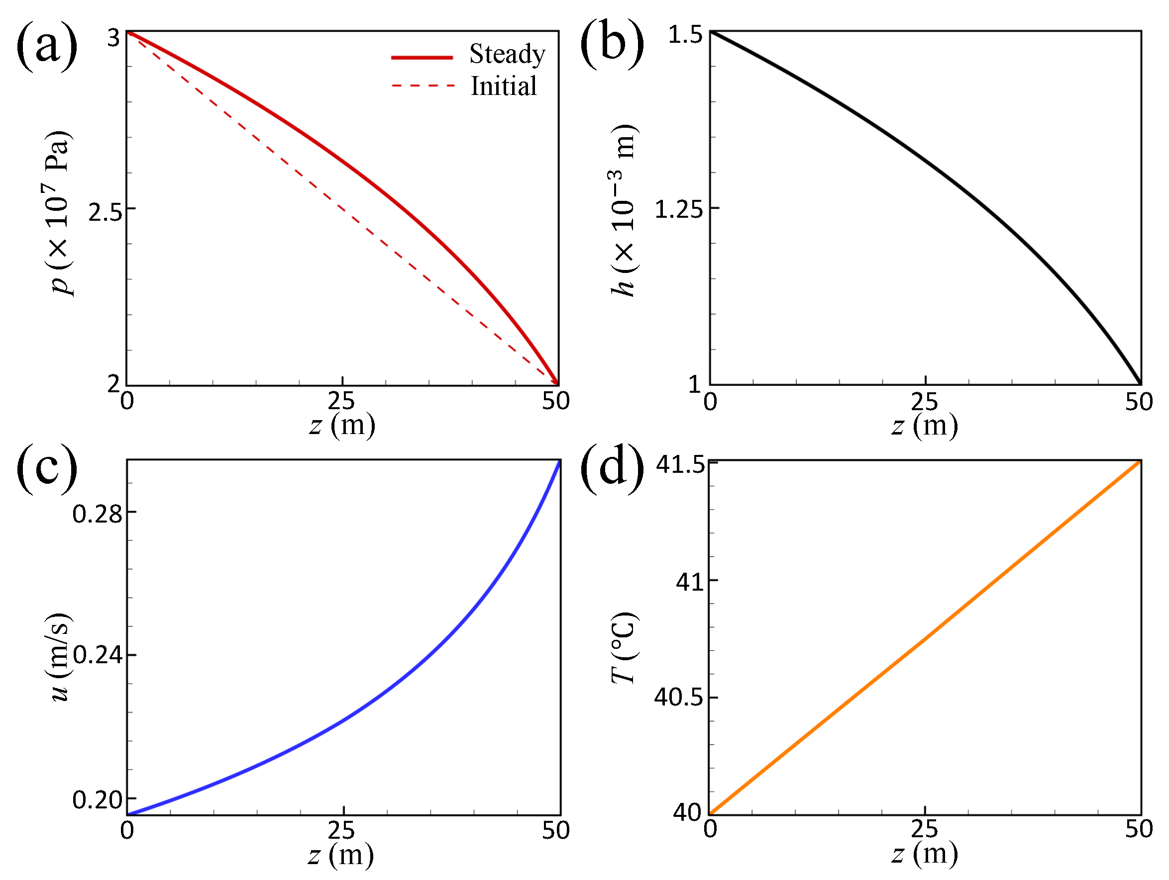
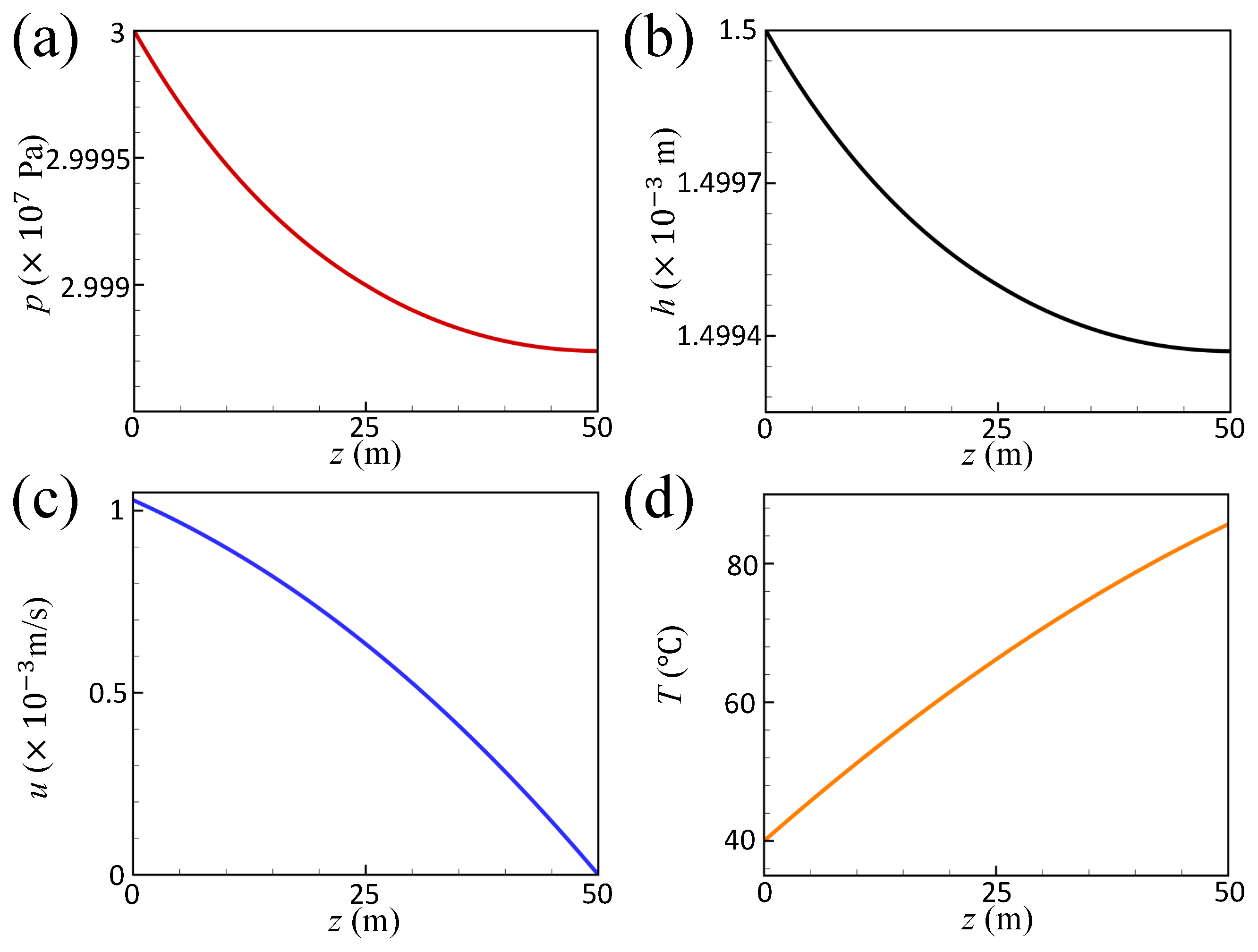
Figure 4 shows the profiles of (a) the liquid pressure, (b) the fracture aperture, (c) the liquid velocity, and (d) the liquid temperature in an open fracture in the steady state. The steady values of the liquid pressure and fracture aperture decrease along the fracture length. As the flux is constant through the fracture based on mass conservation, the liquid speed increases from the inlet to the outlet, which leads to the increasing pressure gradient as shown in (a). According to the positive correlation between the pressure and the leakage speed (Equation (6)), the leakage speed decreases in the vertical direction, along with the pressure. In addition, the leakage speed is around 10−9 m/s in this case, approximately eight orders of magnitude lower than the liquid speed. The large difference between the liquid speed and the leakage speed causes a large value of the length scale, , in Equation (13), making the difference between the liquid temperature and inlet temperature small (according to Equation (12)). Figure 4d shows that the liquid temperature is very close to the inlet temperature, although it slightly increases along the fracture length, suggesting that the temperature of the rock matrix is not important in an open fracture.
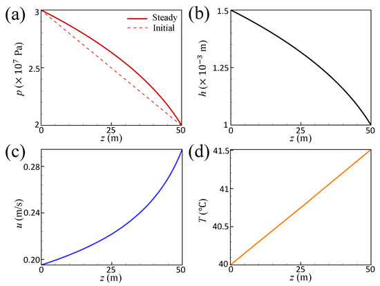
Figure 4.
(a) The pressure profile, (b) the fracture aperture profile, (c) the velocity profile, and (d) the temperature profile in an open fracture. In panel (a), the solid line represents the steady state while the dashed line is the initial profile.
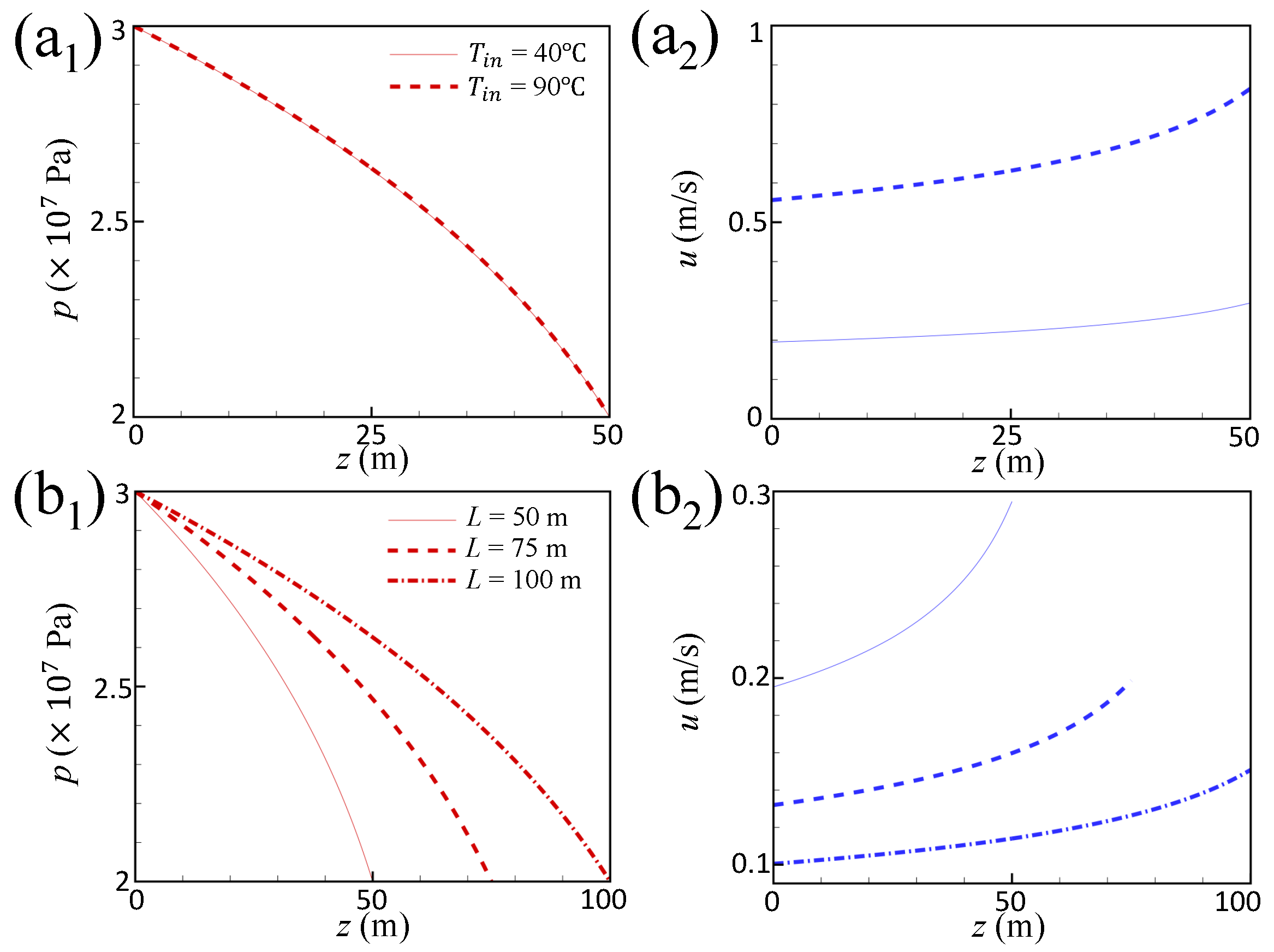
The inlet temperature decides the liquid temperature, hence also decides the liquid viscosity in the fracture. Figure 5(a1,a2) shows that, although the inlet temperature does not obviously affect the pressure profile when it increases from 40 °C to 90 °C (a1), it increases the liquid speed due to the liquid viscosity decreases (a2). However, the ratio of the outlet speed to the inlet speed approximately keeps constant as 1.5, because the speed ratio relates to the aperture ratio and the inlet temperature never alters the fracture aperture at the inlet and outlet. The fracture length also does not change the inlet and outlet apertures, but it does alter the pressure profile in the fracture. Figure 5(b1) shows that the pressure gradient is lower in the longer fracture. Therefore, the liquid speed in the longer fracture is lower, as shown in Figure 5(b2).
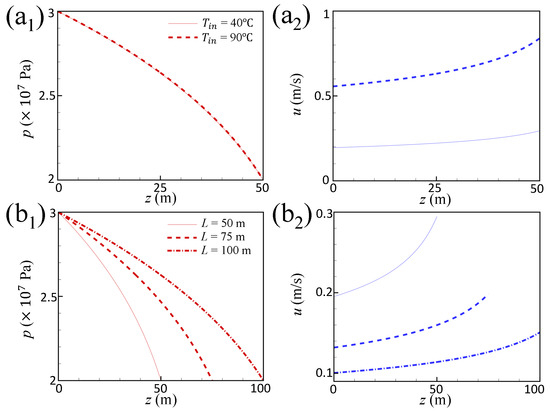
Figure 5.
The profiles of pressure and speed with different inlet temperatures (a1,a2) and different fracture lengths (b1,b2) in an open fracture. The red and blue colors, respectively, represent the pressure and speed profiles.
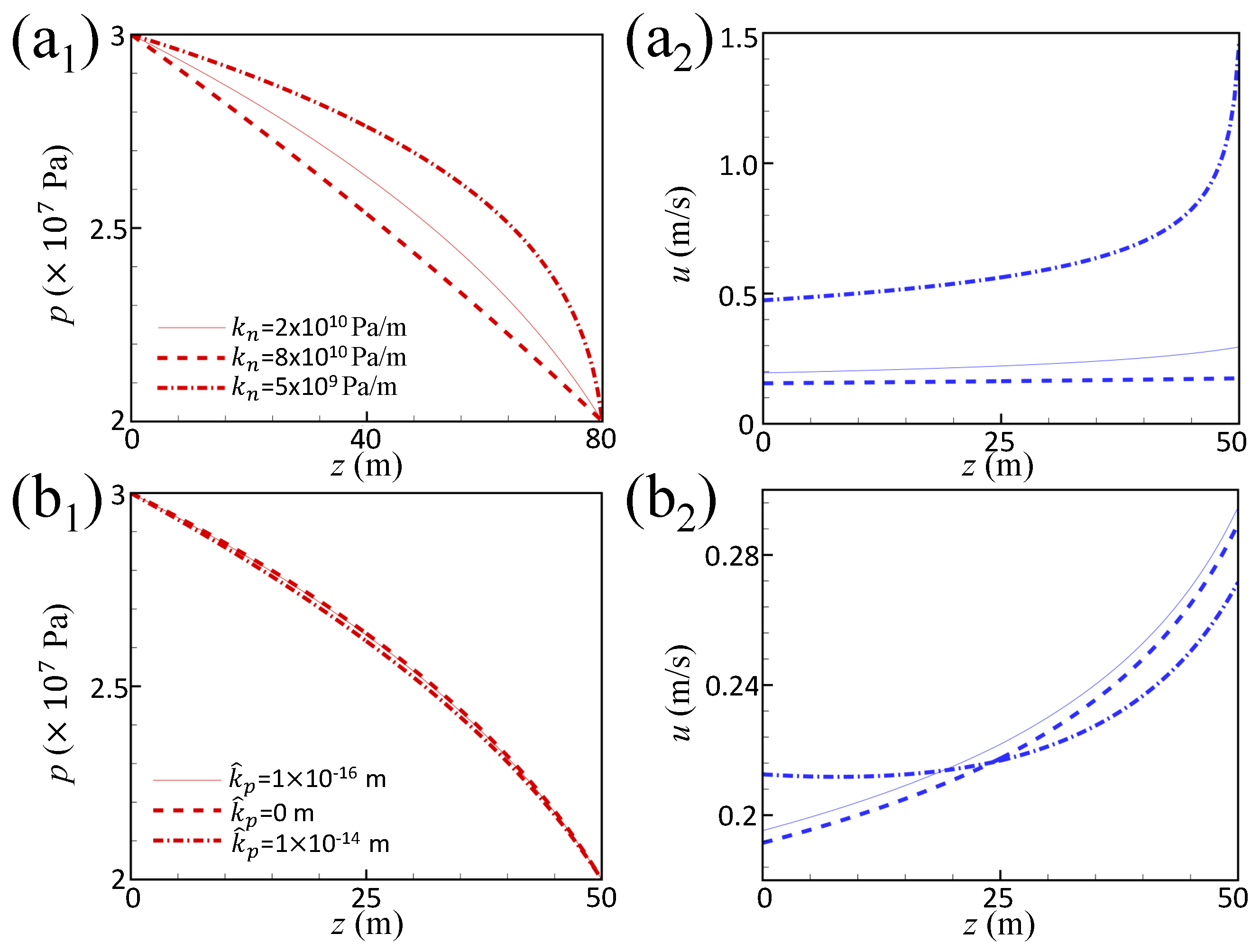
The properties of the rock matrix also play an important role in the flow dynamics of the fracture. Figure 6(a1) shows that the pressure profile is straighter and the interior pressure value is lower for a higher rock stiffness. Unlike the properties of the liquid, the stiffness of the rock can change the aperture of the fracture. According to Equation (17), the larger stiffness and lower interior pressure should lead to a smaller aperture, which agrees with the experimental study by Lai et al. [24]. Figure 6(a2) shows that both the liquid speed and its gradient decrease with increasing stiffness, suggesting an increase in the resistance. Moreover, the ratio of the outlet speed to the inlet speed also decreases with increasing stiffness as a result of the increasing ratio between the outlet and inlet apertures.
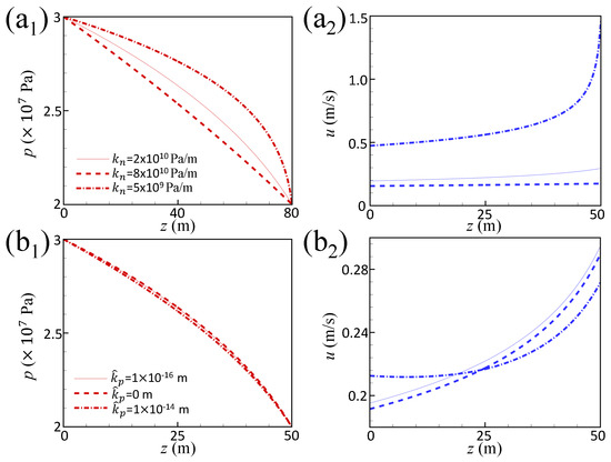
Figure 6.
The profiles of the pressure and speed with different rock stiffnesses (a1,a3) and different rock permeabilities (b1,b2) in an open fracture. The red and blue colors, respectively, represent the pressure and speed profiles.
Figure 6(b1) shows the effect of the permeability on the pressure profile, and indicates that the pressure profile is straighter and the interior pressure is slightly lower at a higher permeability. The change in the speed profile with the permeability is more obvious than that of the pressure profile. As shown in Figure 6(b2), the liquid speed at a permeability of 10−16 m is higher than that without any permeability. The reason for the higher liquid speed is that the viscosity of the liquid is higher with a finite permeability. According to Equations (12) and (13), the liquid temperature increases when the leakage velocity, , increases from zero to a finite value, which then increases the liquid viscosity. As the permeability increases from 10−16 m to 10−14 m, the inlet speed continuously increases but the outlet speed decreases, due to the increasing volume of liquid leaving through leakage.
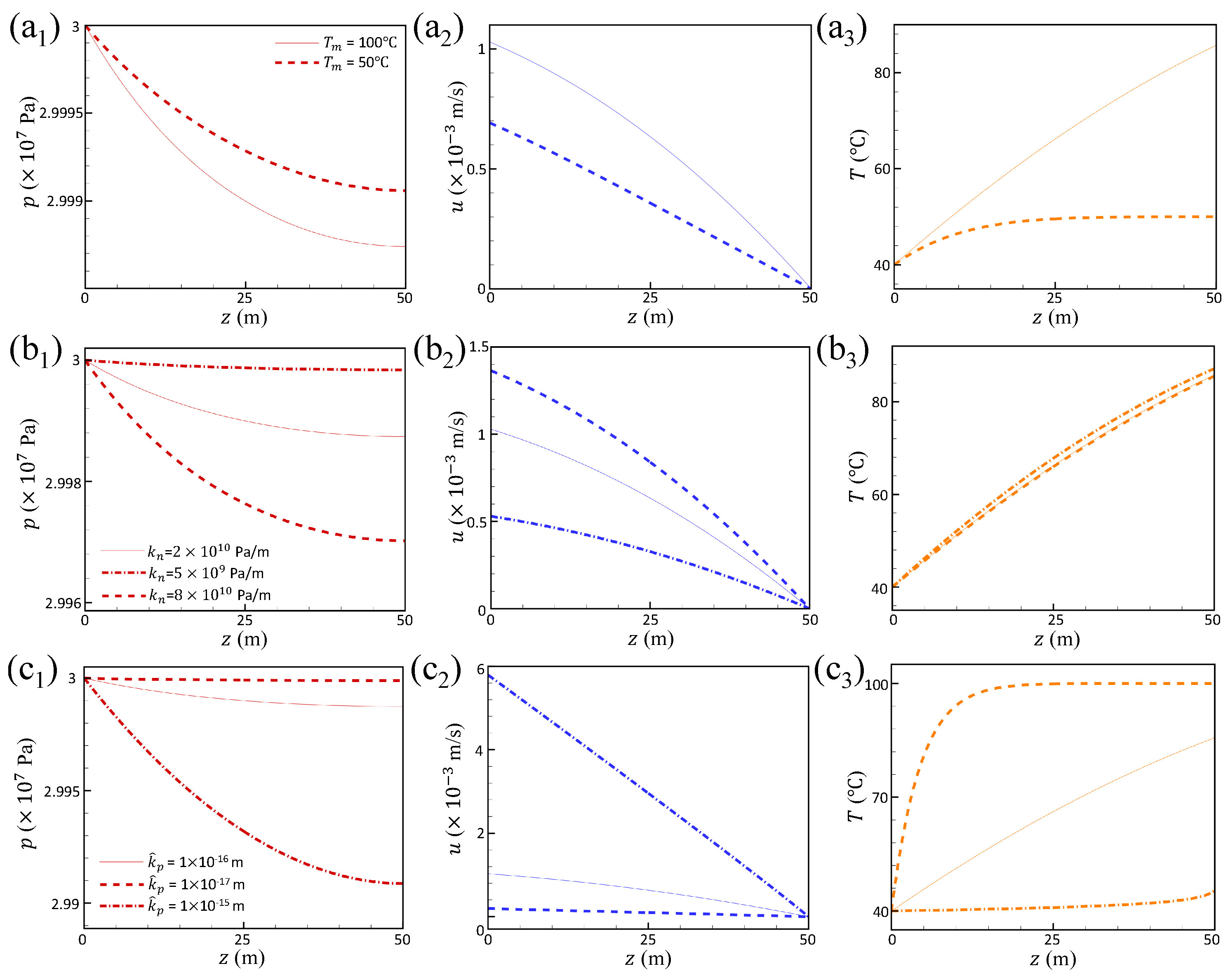
Figure 7 shows the steady profiles of (a) liquid pressure, (b) fracture aperture, (c) liquid speed, and (d) liquid temperature in a closed fracture with . The used parameters are listed in Table 1. Compared with the results shown in Figure 4, the liquid pressure and fracture aperture change slightly from the inlet to the outlet (a,b), and the liquid speed is more than two orders of magnitude lower than that in the open fracture (c). Moreover, the liquid temperature is higher (d) than that in the open fracture. The reason for the higher liquid temperature is the higher ratio of the leakage speed to the liquid speed. In a closed fracture, the speed ratio is more than two orders of magnitudes higher than that in the open fracture. The higher speed ratio leads to the lower value of length scale in Equation (12), thus increasing the effect of the rock matrix temperature on the liquid temperature.
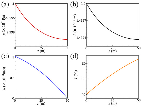
Figure 7.
(a) The steady pressure profile; (b) the fracture aperture profile; (c) the velocity profile; and (d) the temperature profile in a closed fracture with .
Figure 8 further presents the effects of rock properties, including the rock matrix temperature, stiffness, and permeability, on the dynamics and temperature of the liquid in a closed fracture. (a1,a2) show that the pressure gradient and the liquid speed are lower at the lower rock matrix temperature, due to the higher viscosity of the liquid. The lower rock temperature causes a lower liquid temperature (a3), and hence a higher liquid viscosity. (b1) shows that the interior pressure is higher but the pressure gradient is lower at the lower rock stiffness. The lower pressure gradient leads to a lower liquid speed in the fracture, as shown in (b2). The liquid temperature is slightly lower at the higher stiffness (b3), as the higher liquid speed strengthens the heat transfer. This finding agrees well with the theoretical and numerical studies proposed by Wang et al. [38], in that the temperature of the liquid in the fracture decreases with the faster flow. (c1,c2) show that the permeability plays a similar role in the pressure and speed profiles on the stiffness, suggesting that the pressure gradient and the interior speed increase with increasing permeability, which is in agreement with the study by Detournay and Garagash [39] on the near-tip region of a fluid-driven fracture. The permeability also alters the liquid temperature. (c3) presents that the liquid temperature is closer to the rock temperature at lower permeability, owing to the lower liquid speed.
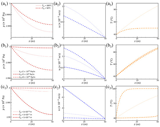
Figure 8.
The profiles of the pressure, speed, and temperature with different rock matrix temperatures (a1–a3), rock stiffnesses (b1–b3), and rock permeabilities (c1–c3) in a closed fracture. The red, blue, and orange colors, respectively, represent the pressure, speed, and temperature profiles.
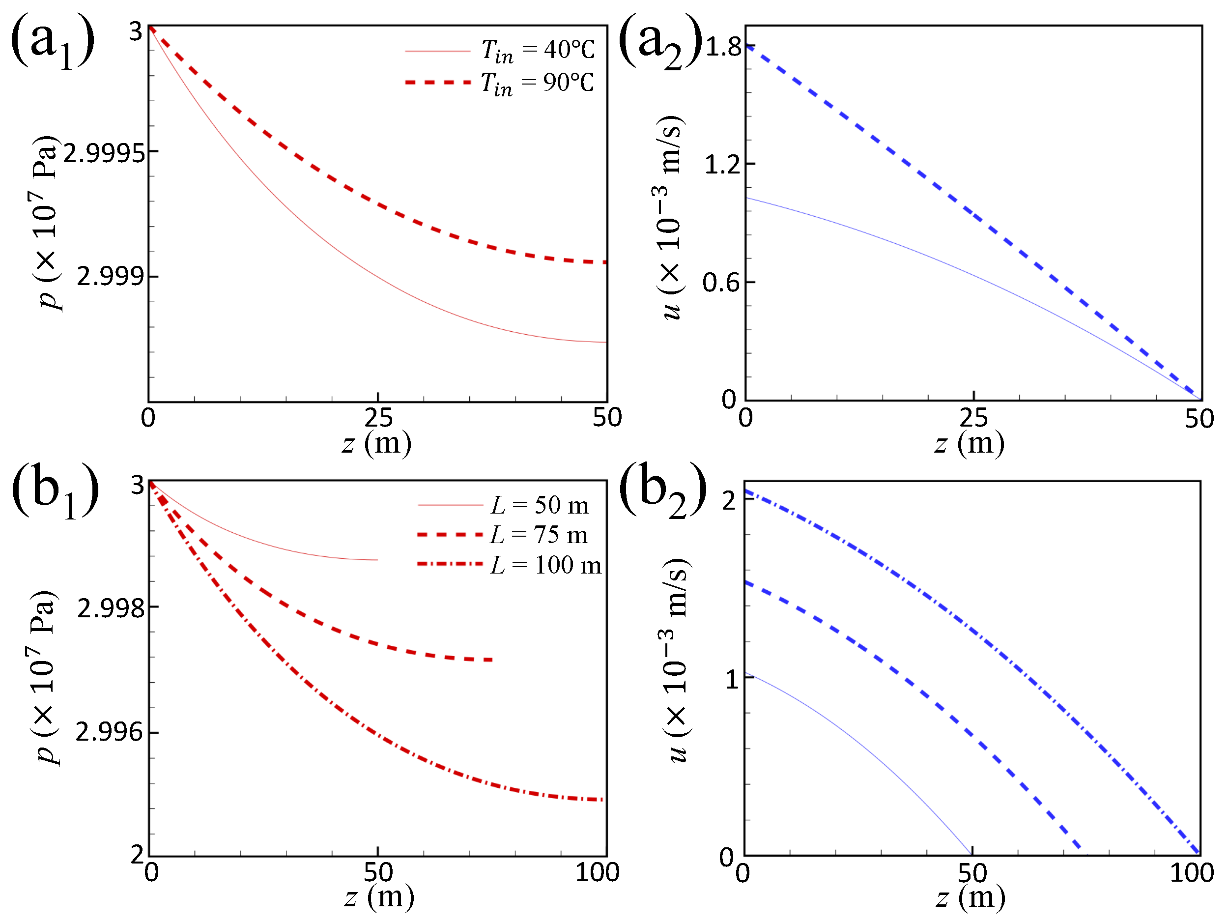
The parameters of the fracture also have significant effect on the liquid flow. Figure 9(a1,a2) shows that an increase in the inflow temperature reduces the pressure gradient but increases the interior speed for a liquid in a closed fracture due to the decreasing liquid viscosity. Figure 9(b1,b2) shows that the higher value of the fracture length L leads to a higher pressure gradient and lower interior pressure, as well as a higher liquid speed. It is different from the case in an open fracture (Figure 5(b1,b2)), owing to the greater importance of the leakage in a closed fracture. More leakage occurs in a longer fracture, leading to a higher inlet speed and hence a higher interior speed.
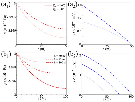
Figure 9.
The profiles of the pressure and speed with different inlet temperature (a1,a2) and different fracture length (b1,b2) in a closed fracture with . The red and blue colors, respectively, represent the pressure and speed profiles.
We then evaluate the effect of the propagating speed of the outlet, , on the fluid flow in a closed fracture. As shown in Figure 10, the gradient of the pressure increases with the propagating speed (a), which is consistent with the increasing liquid speed (b). This suggests that the growth of the fracture increases the pressure difference between the inlet and outlet, and also promotes flow in the fracture. The higher liquid speed hence increases the effect of the inlet temperature on the liquid temperature at the higher value of , thereby reducing the liquid temperature in the fracture (c).
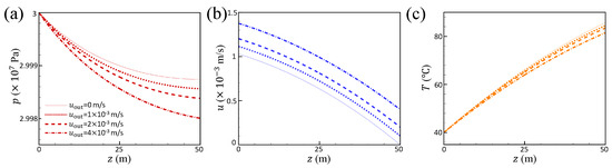
Figure 10.
The profiles of (a) the liquid pressure, (b) the liquid speed, and (c) the liquid temperature in the closed fractures with different propagating speeds.
3. The Upward Flow of Liquid in a Bifurcated Fracture
In this section, we further consider the liquid flow in a bifurcated fracture with three connected channels. Our main objective is to investigate how the changing of the parameters in the channels alters the liquid flow in the bifurcated fracture.
3.1. Model
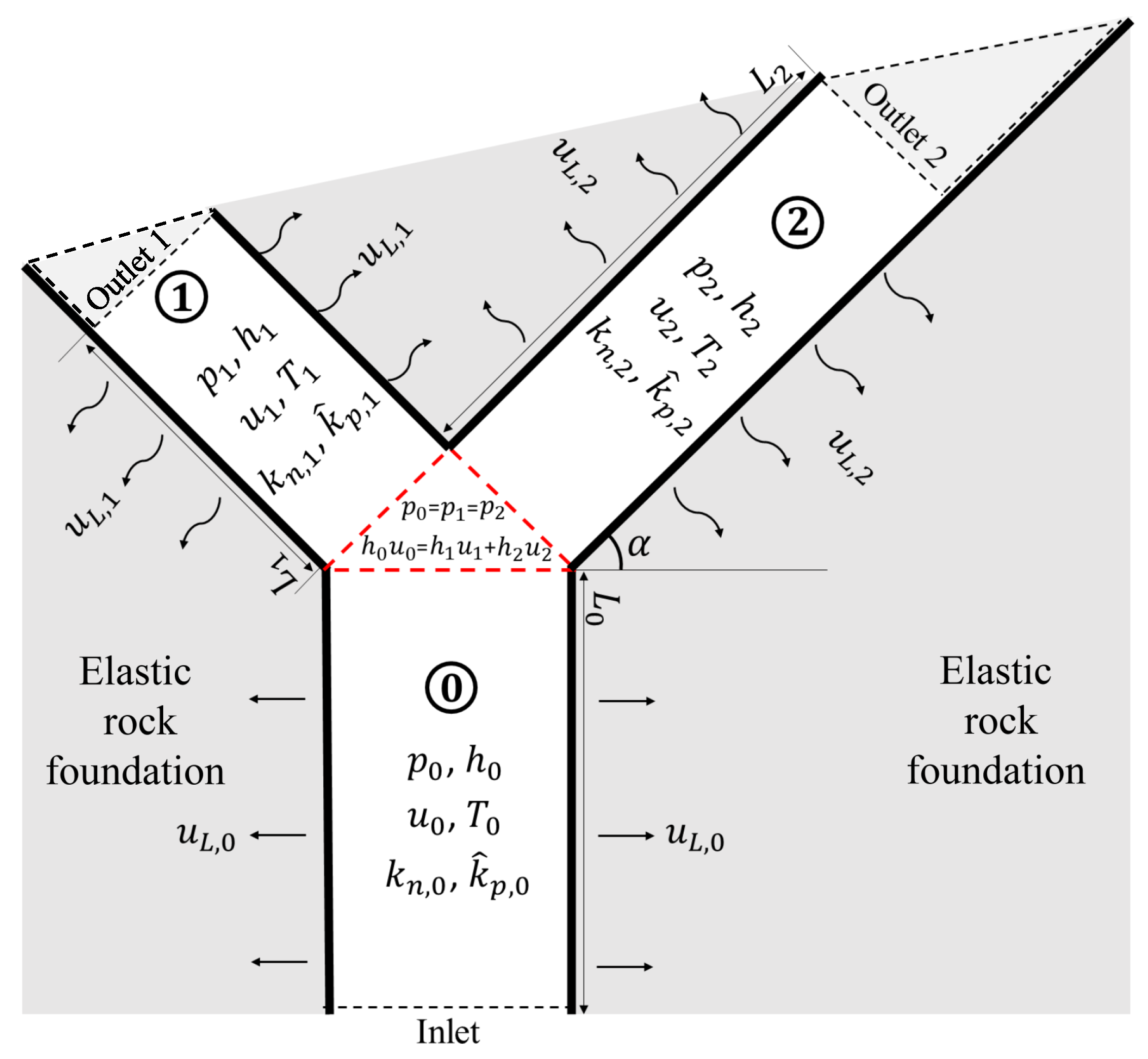
Figure 11 illustrates our model, where the liquid flows from channel 0 (the main channel) to channels 1 and 2 (the branches). Our model allows the parameters of these three channels to differ from each other. Similar to the case of flow in the single fracture, we assume the angle to be 90 degrees, and ignore the gravity term because it is negligible compared with the pressure term.
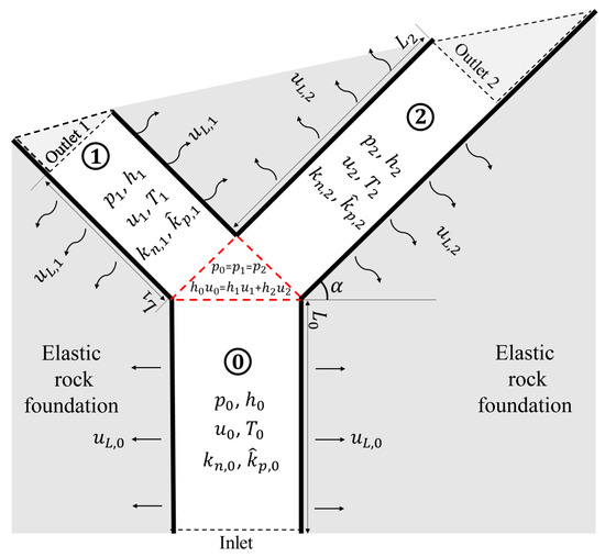
Figure 11.
Model of a branch fracture consisting of channels 0, 1, and 2. For an open channel, the triangles surrounded by the dashed line are removed from the outlets of channels 1 and 2, while, for the closed channel, the triangles remain.
3.1.1. Governing Equations
In channels 0, 1, and 2, we describe the evolution of the fracture aperture using the following nonlinear equations, respectively,
where the subscripts 0, 1, and 2 represent the variables in channels 0, 1, and 2, and the leakage speeds in the channels can be computed as follows,
Based on the balance between the elastic force and the liquid pressure, we describe the relationship between the fracture aperture and the pressure in the three channels as follows,
3.1.2. The Boundary and Initial Conditions
Solving the governing equation requires suitable boundary conditions. At the connection of the channels (marked by a red dashed line in Figure 11), the liquid pressure is homogeneous, as
Meanwhile, the channel apertures and liquid speeds satisfy the following correlation,
according to mass conservation. Using Equation (26), our model allows the apertures and speeds in channels 1 and 2 to be different. It is worth mentioning that, because of this case of velocity discontinuity, the analysis based on the tridiagonal solver is restricted to symmetrically distributed cases.
The inlet of the main channel, channel 0, is the entrance of the whole bifurcated fracture, where we set a Dirichlet boundary condition for the pressure as
Similar to the case of the single fracture, we define “open” and “closed” outlets for the branches, either channel 1 or channel 2. At the open outlet, we set a constant pressure, , as
We impose a constant speed, , at the closed outlet, so the gradient of the pressure is
At the beginning of all computations, we again define the initial pressure to decrease linearly from to in the bifurcated fracture.
3.2. Results
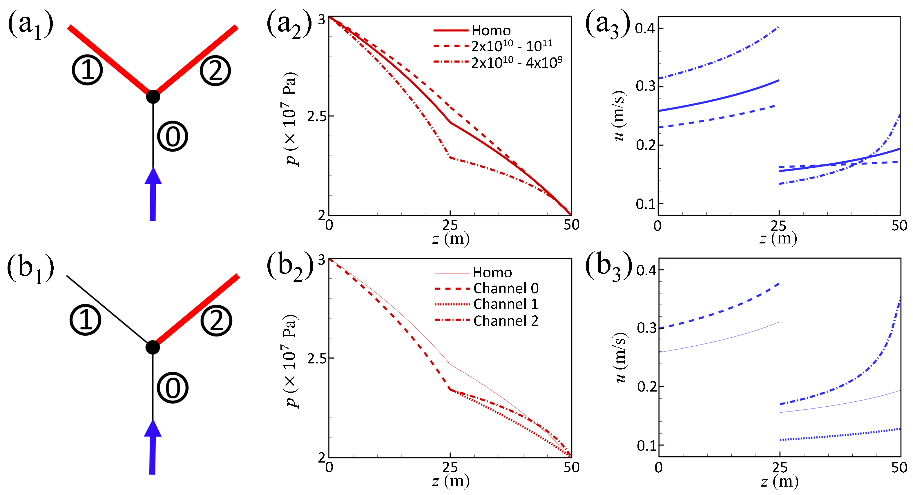
We first evaluate the role of the rock stiffness on the flow in the open bifurcated fracture with the boundary condition at the outlets defined by Equation (28). We assume the stiffness of the branches (channels 1 and 2) to be the same as shown in Figure 12(a1–a3), which shows the effect of the changing stiffness from the main channel (channel 0) to the branches (channels 1 and 2) on the pressure and speed profiles. Compared with the single fracture (as shown in Figure 4), both the pressure gradient and speed vary sharply at the connection of the channels in the bifurcated fracture due to the flow diversion. If the stiffness of the branches is higher than that of the main channel, the pressure at the channel connection increases ((a2)), but the inlet and outlet speeds of the bifurcated fracture decrease ((a2)) because of the reduced pressure gradient at the inlet and outlet.
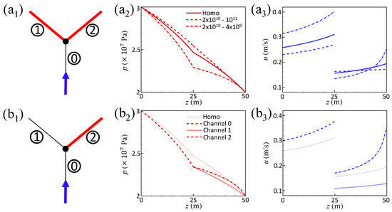
Figure 12.
(a1) illustrates the bifurcated fracture when channels 1 and 2 have the same parameters. (a2,a3), respectively, compare the profiles of the pressure and speed in an open bifurcated fracture with homogeneous stiffness (2 × 10¹⁰ Pa/m) with those in open bifurcation fractures, where the stiffness of channels 1 and 2 is higher (2 × 10¹¹ Pa/m) or lower (4 × 10⁹ Pa/m) than that of channel 0 (2 × 10¹⁰ Pa/m). (b1) illustrates a bifurcated fracture in which channel 2 has different parameters from channels 0 and 1. (b2,b3), respectively, present the profiles of the pressure and speed in the open bifurcated fractures, where the stiffness of channel 2 is 4 × 10⁹ Pa/m but that of channels 0 and 1 is 2 Pa/m. For comparison, we plot the profiles in the bifurcated fracture with the homogeneous stiffness as light lines.
We also investigate the flow dynamics in the bifurcated fracture when the stiffness of channel 2 is lower than that of channels 0 and 1, as shown in Figure 12(b1). Figure 12(b2,b3) shows that the lower stiffness of channel 2 causes a higher interior pressure and higher speed than that of channel 1, which is in agreement with the case of a single channel (Figure 6(a1,a2)). Moreover, the lower stiffness in channel 2 reduces the interior pressure in channels 0 and 1. It also increases the pressure gradient at the inlet of channel 0 while decreasing the pressure gradient at the outlet of channel 1 ((b2)), hence increasing the inlet speed but decreasing the speed at the outlet ((b3)).
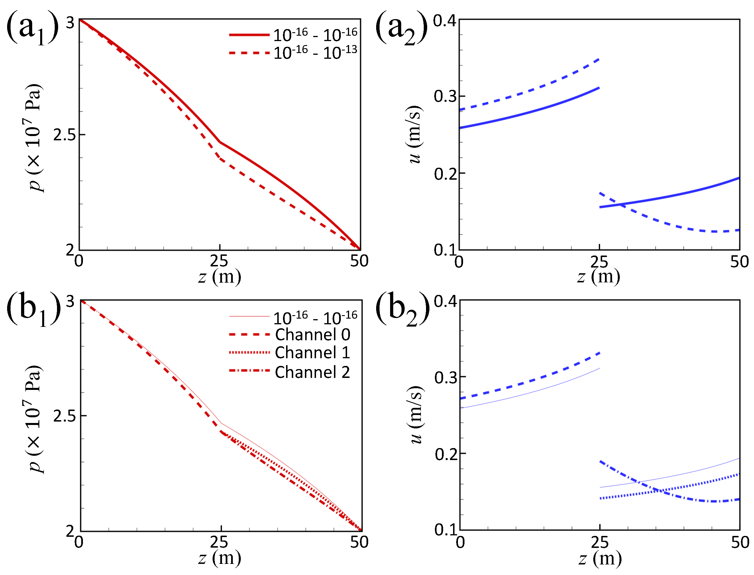
The permeability also affects the flow in the open bifurcated fracture. Figure 13(a1) compares the pressure profiles between a fracture with homogeneous permeability and a fracture in which the permeabilities of channels 1 and 2 are equal and higher than the permeability of channel 0, and suggests that the high permeability of channels 1 and 2 reduces the interior pressure in the whole fracture. Due to the increased pressure gradient at the inlet, the inlet speed of the fracture is higher than that with homogeneous permeability, as shown in Figure 13(a2). The outlet speed, however, becomes lower, as a result of the increased leakage through the wall of the fracture.
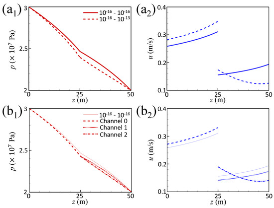
Figure 13.
(a1,a2), respectively, show the profiles of the pressure and speed in the open bifurcated fractures, where the permeabilities of the channels 1 and 2 are the same. The solid line presents the case in which the permeability of the three channels is homogeneous at m. The dashed line represents the case in which the permeability of channel 0 ( m) is lower than that of channels 1 and 2 ( m). (b1,b2), respectively, show the profiles of the pressure and speed in the bifurcated fractures, where the permeabilities of channels 0 and 1 ( m) are lower than that of channel 2 ( m). The dashed, dotted, and dashed–dotted lines represent channels 0, 1, and 2, respectively. As a comparison, we plot the case of homogeneous rock stiffness ( m) as a light solid line.
Figure 13(b1,b2) shows the profiles of the pressure and speed, respectively, when the permeability of channel 2 is higher than that of channels 0 and 1. The higher permeability of channel 2 reduces the interior pressure in all three channels ((b1)), and causes a higher speed in channel 0 than that with homogeneous permeability ((b2)) because of the increased pressure gradient. The inlet speed of channel 2 is higher than that of channel 1, suggesting that more liquid flows into channel 2. This reduces liquid speed in channel 1. The outlet speed of channel 2, however, is lower than that of channel 1, as a result of the higher leakage.
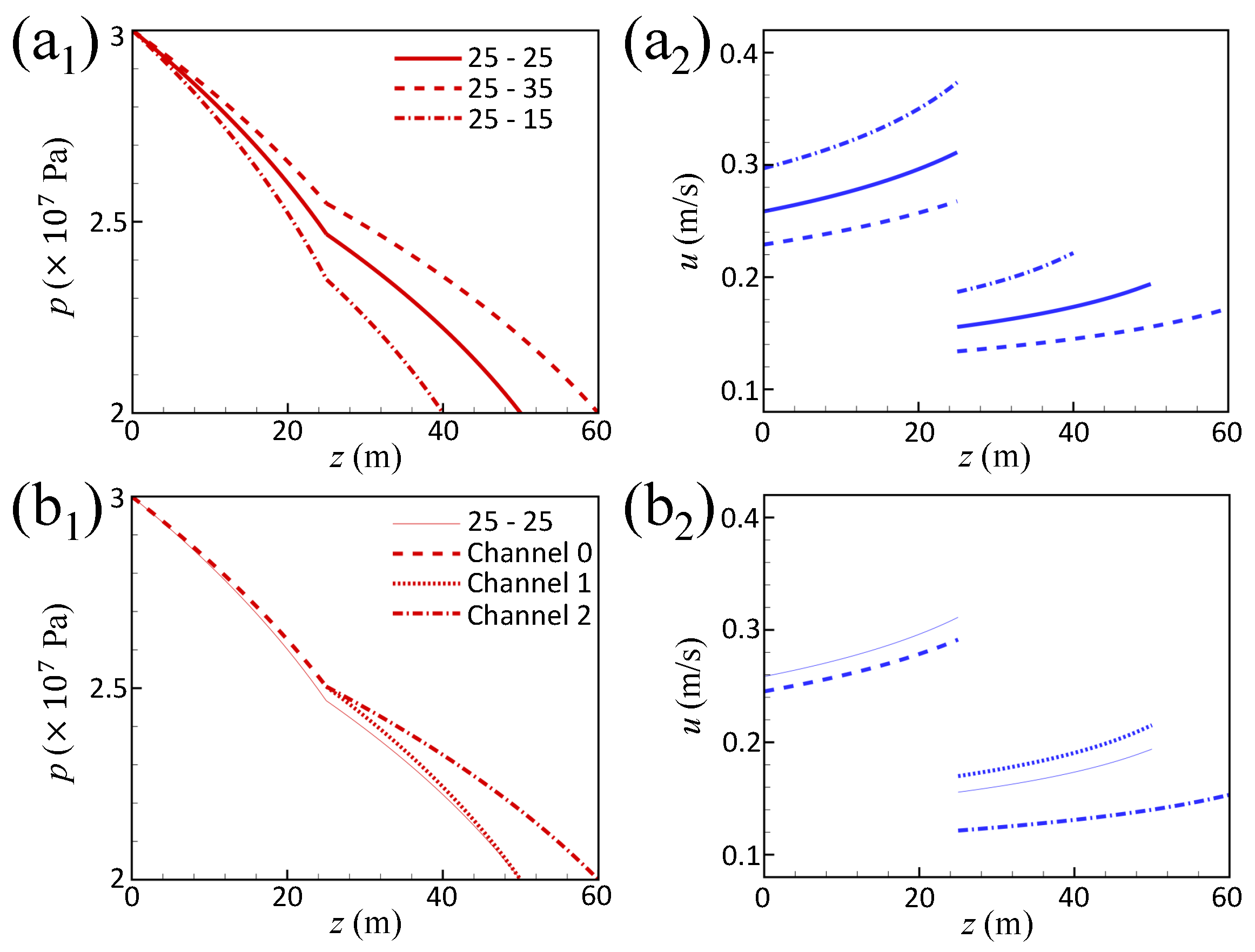
The last parameter we investigate for the open bifurcated fracture is the channel length. Figure 14(a1,a2) shows that increasing the length of channels 1 and 2 increases the interior pressure but reduces the speed in the whole fracture, as a result of the decreasing pressure gradient. When the length of channel 2 increases to a higher value than the lengths of channels 0 and 1, the interior pressure increases but the pressure gradient decreases in channel 0, as shown in Figure 14(b1). The lower pressure gradient leads to a lower speed in channel 0. The higher length of channel 2 also causes a lower pressure gradient and lower speed than channel 1, implying that more liquid flows into channel 1. Therefore, the speed in channel 1 is higher than that with a homogeneous length.
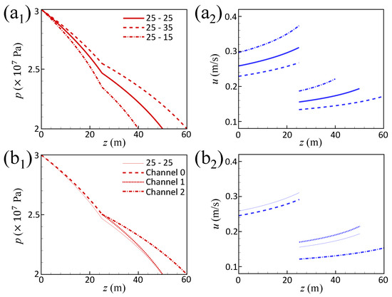
Figure 14.
(a1,a2), respectively, show the profiles of the pressure and speed in the open bifurcated fractures, where the lengths of channels 1 and 2 are the same. The solid line represents the case in which the length of channel 0 is the same as that in channels 1 and 2, which is 25 m. The dashed and dashed–dotted lines, respectively, represent the case in which the length of channel 0, 25 m, is lower and higher than that of channels 1 and 2, 15 m and 35 m. (b1,b2), respectively, show the profiles of the pressure and speed in the bifurcated fractures, in which the lengths of channels 0 and 1 (25 m) are smaller than that of channel 2 (35 m). The dashed, dotted, and dashed–dotted lines represent channels 0, 1, and 2, respectively. As a comparison, we plot the case of the homogeneous channel length (25 m) as a light solid line.
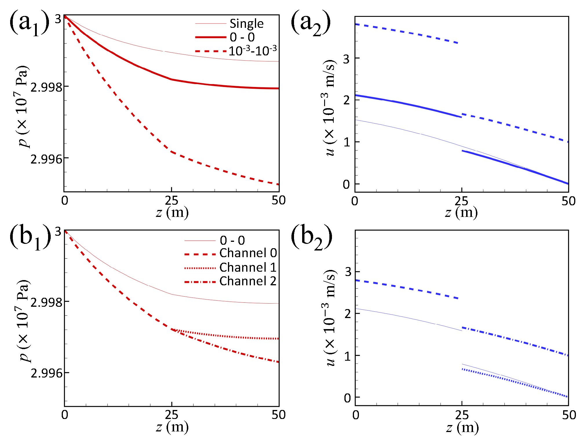
We then investigate the flow dynamics in the closed bifurcated fracture, where the boundary condition at the outlets is defined by Equation (29). As shown in Figure 15(a1), the interior pressure and the outlet pressure are lower in the bifurcated fracture with equal propagating speeds, , than the single closed fracture, due to more leakage through the wall of the three channels. Moreover, the pressure decreases, but the pressure gradient increases with the increasing propagating speeds of channels 1 and 2. The higher pressure gradient at the higher propagating speed leads to a higher speed in the bifurcated fracture, as shown in (a2). The individual changing of the propagating speed in channel 2 also alters the profiles. Figure 15(b1) shows that the interior pressure of the bifurcated fracture decreases if the propagating speed of channel 1 is zero but that of channel 2 is 10−3 m/s. The higher propagating speed also causes a lower interior pressure but a higher pressure gradient in channel 2 than in channel 1. Figure 15(b2) shows the speed profiles with the unequal propagating speeds, suggesting that the increasing propagating speed increases the interior speed of channel 2 as well as that of channel 0, which is consistent with the increasing pressure gradient shown in (b1).

Figure 15.
(a1,a2), respectively, present the profiles of the pressure and speed in the closed bifurcated fractures, where the propagating speeds of channels 1 and 2 are the same. The solid line represents the case in which = 0, while the dashed line represents the case with = 10−3 m/s. As a comparison, we plot the profiles in single closed fracture as a light solid line. (b1,b2), respectively, present the pressure and speed profiles in the closed bifurcated fractures, in which the propagating speed of channel 1 is zero but that of channel 2 is 10−3 m/s. As a comparison, we plot the case of the homogeneous propagating speed (zero) as a light solid line.
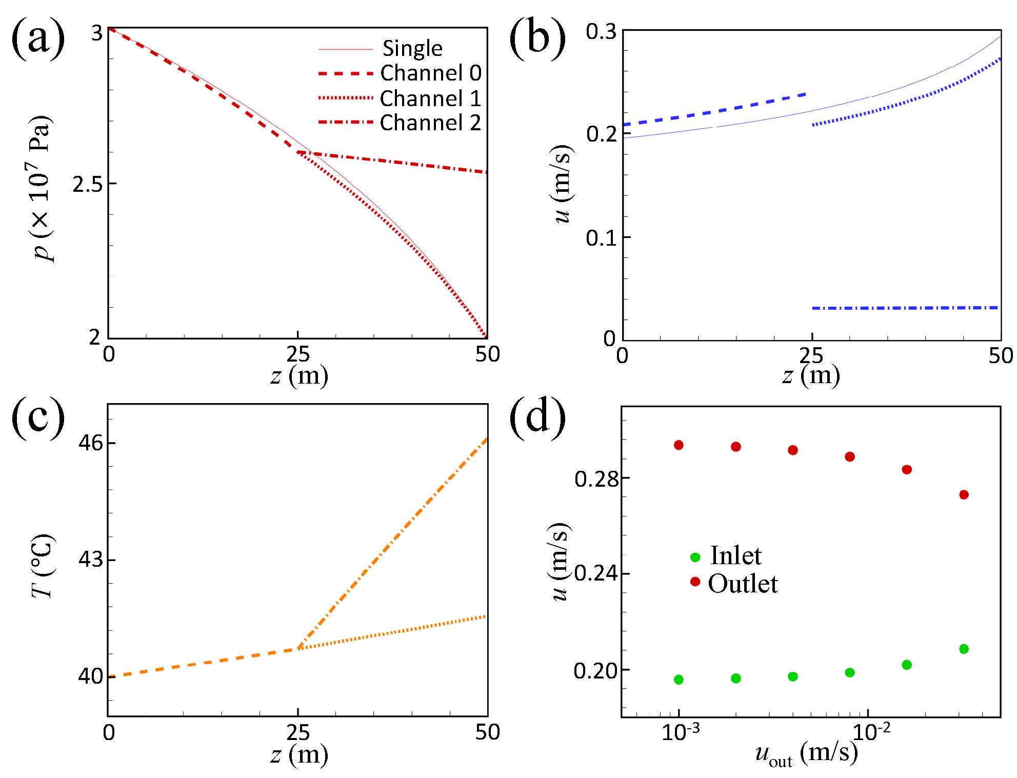
Figure 16a shows the pressure profile in the bifurcated fracture with an open channel 1 and a closed channel 2, where the imposed propagating speed of channel 2 is 0.032 m/s. Compared with the single fracture, the existence of channel 2 decreases the interior pressure in channels 0 and 1. Channel 2 also changes the speed profile in the fracture, leading to the speed in channel 0 being higher than that in the first half of the single fracture, while also causing a lower speed in channel 1. In channel 2, the speed is approximately constant and lower than that in channels 0 and 1, which is consistent with the lower pressure gradient in channel 2 (as shown in (a)). The lower speed in channel 2 weakens the heat transfer from the inlet of the fracture, and therefore the temperature of the flow in channel 2 is higher than that in channel 1, as shown in (c). Figure 16d shows that the increasing propagating speed of channel 2 reduces the outlet speed of channel 1, although it increases the inlet speed of channel 0.
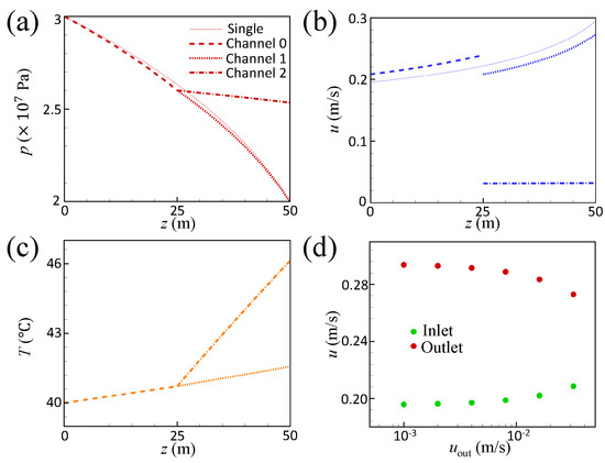
Figure 16.
(a–c), respectively, show the profiles of the pressure, speed, and temperature in the bifurcated fractures, where channel 1 is open but channel 2 is closed, with a propagating speed of 0.032 m/s. The dashed, dotted, and dashed–dotted lines represent channels 0, 1, and 2, respectively. For comparison, we plot the profiles of a single fracture as a light solid line. (d) The variation of the inlet speed of channel 0 (green circles) and outlet speed of channel 1 (brown circles) with the given propagating speed of channel 2.
4. The Upward Flow in a Fracture Network
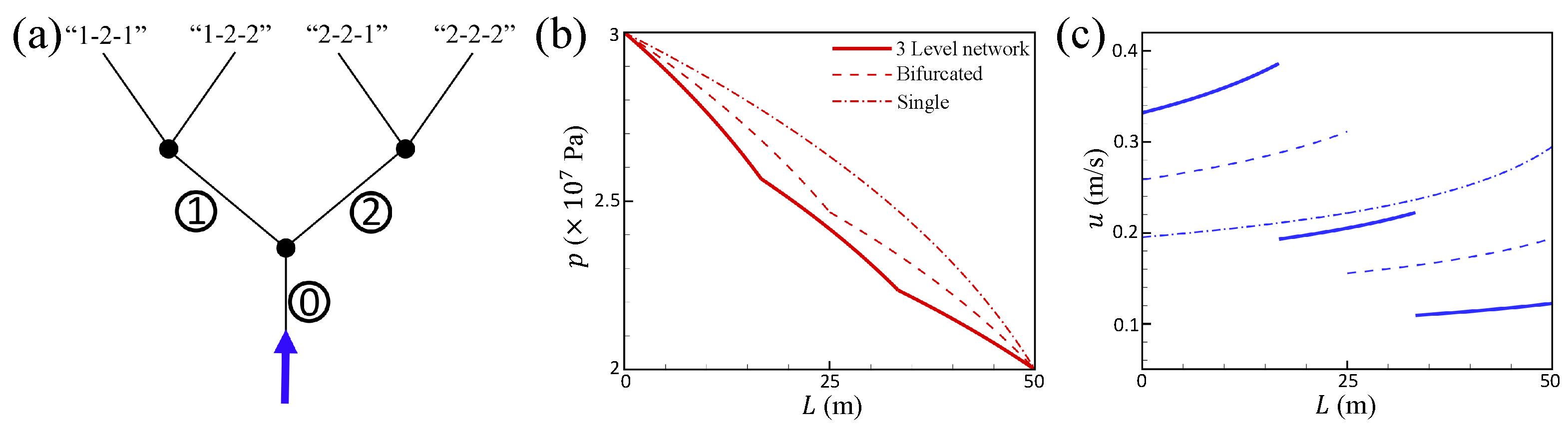
We finally generalize our model to a fracture network of n levels involving 2n−1− 1 channels and 2n− 1 connections, as shown in Figure 17. The network on levels 0 and 1 is the same as the bifurcated fracture shown in Figure 11, where channels 1 and 2 are connected to channel 0. Above level 1, the channels are divided into two categories. The channels of the first category derive from channel 1, named “1-n-x”, where “x” = 1, 2, …, 2n−1 represents the index of the channel on level n. The second category originates from channel 2, and thus the channels are named as “2-n-x”.
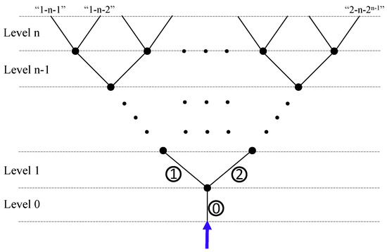
Figure 17.
Model of a fracture network of n levels.
4.1. Model
Our model of the fracture network is similar to that of the bifurcated fracture in Section 3.1 but with more governing equations and initial and boundary conditions.
4.1.1. Governing Equation
The governing equations are again,
and
and
The i indicates the channel label. For level 0 and level 1 channels, i is 0, 1, and 2, respectively. For channels of level 2 and above, the i of the channels from channel 1 of level 1 is 1-n-1, 1-n-2, …, 1-n-2n−1. The i of the channels from channel 2 of level 1 is 2-n-1, 2-n-2, …, 2-n-2n−1.
By solving these equations, we expect to capture the pressures, velocities, and apertures for all channels.
4.1.2. The Boundary and Initial Condition
Similarly to the case of the bifurcated fracture, we set the liquid pressure to be homogeneous at each connection. As an example, we set
at the first connection on level , same as the three-pronged crack due to conservation of mass.
We set a Dirichlet boundary condition for the pressure at the inlet of channel 0, which is also the entrance of the whole fracture network, as
As shown in Figure 17, the fracture network involves 2n outlets, which are also the outlets of the 2n channels on level n. Similar to the single and bifurcated fractures, we define “open” and “closed” outlets for the channels on level n. For example, assuming the length of the outlet of channel 1-n-1 to be , we set a constant pressure, , there to create an open outlet as
To set a closed outlet for channel 1-n-1, we impose a constant speed, , there, so that the gradient of the pressure is
Similar to the cases of single and bifurcated fractures, the initial pressure in the fracture network decreases linearly from to at the beginning of all computations shown in the following section.
4.2. Result
In this study, we focus on the dynamics of the upward flow in a 3-level fracture network, as shown in Figure 18a. At first, we assume the fracture network to be homogeneous, where all seven channels have the same parameters as listed in Table 1. The total length of the fracture is 50 m and all channels have same length. All channels on level 2 have open outlets. Figure 18b compares the pressure profile of the 3-level fracture network to that of the single and bifurcated fractures, suggesting that the interior pressure decreases with an increasing number of levels. Moreover, the inlet pressure gradient is higher while the outlet pressure gradient is lower in the fracture with more levels. As a result, the inlet speed of the fracture increases with the number of levels, whereas the outlet speed decreases, as shown in Figure 18c.
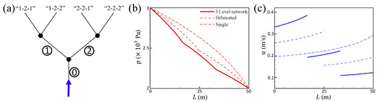
Figure 18.
(a) illustrates the 3-level fracture network with homogeneous parameters and open outlets. (b,c) show the profiles of the pressure and speed in the fracture network, respectively. For comparison, the profiles of the pressure and speed in the single (dashed-0dotted lines) and bifurcated (dashed lines) fracture are also plotted in (b,c).
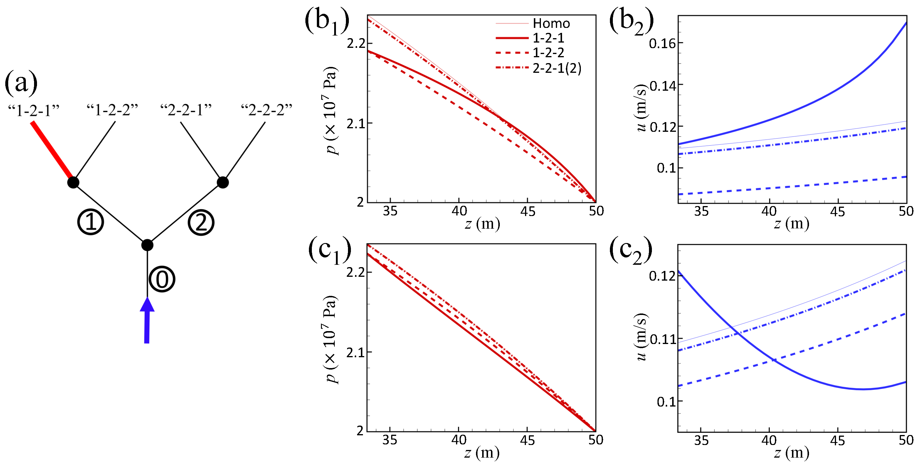
We also investigate the heterogeneous fracture network, as shown in Figure 19a, where a channel on level 2 (i.e., channel 1-2-1) has different parameters from the others. Figure 19(b1) shows that the reduced stiffness of channel 1-2-1 decreases the interior pressure in all other channels on level 2. The interior pressure decreases more in channel 1-2-2 than in channels 2-2-1 and 2-2-2. In agreement with the cases of the single and bifurcated fractures, the speed in channel 1-2-1 increases with the reduced stiffness, as shown in Figure 19(b2). The increased inlet speed of channel 1-2-1 leads to more liquid flowing in, thus decreasing the speed in the other channels on level 2. Similarly to the interior pressure, the speed decreases more in channel 1-2-2 than in channels 2-2-1 and 2-2-2. Figure 19(c1,c2) shows the effect of the increased permeability of channel 1-2-1 on the pressure and speed profiles of the channels on level 2, suggesting that the increased permeability decreases both the interior pressure and speed. Again, the degree of the decrease is larger in channel 1-2-2 than in channels 2-2-1 and 2-2-2. The above results indicate that changing the parameters in a channel leads to a greater effect on the flow dynamics in the closer channels.
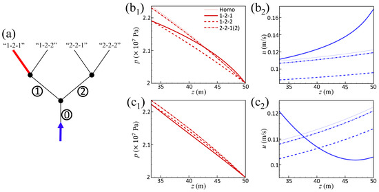
Figure 19.
(a) illustrates the 3-level fracture network in which the parameters of channel 1-2-1 (red line) are different from those of the other channels. (b1,b2), respectively, show the pressure and speed profiles in the channels on level 2 when the stiffness of channel 1-2-1 is at a lower value than that of other channels (4 × 10⁹ Pa/m). (c1,c2), respectively, show the pressure and speed profiles in the channels on level 2 when the permeability of channel 1-2-1 is at a higher value than that of other channels (1 × 10⁻³ m). For comparison, we plot the profiles of the homogeneous fracture network as light lines.
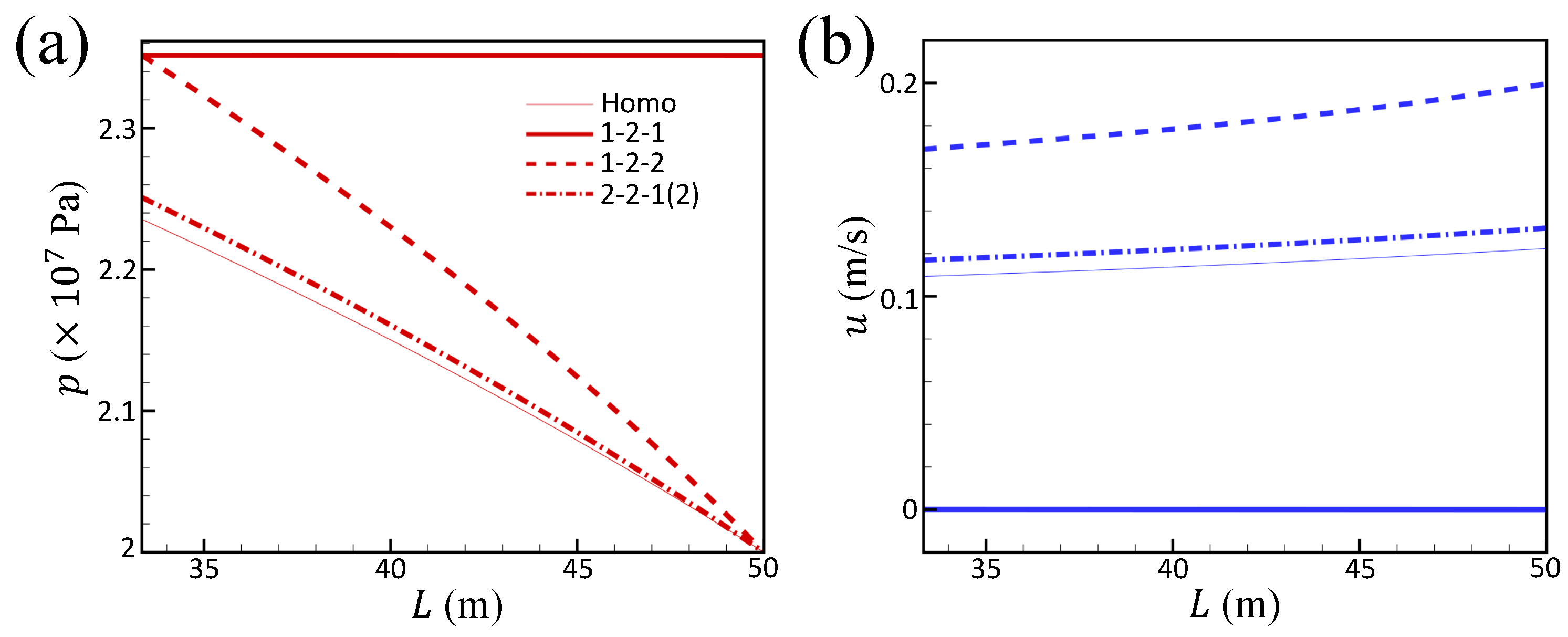
Next, we switch the outlet of channel 1-2-1 from open to closed and set the propagating speed, , to be zero, to study the effect of the heterogeneous boundary condition on the flow dynamics. Figure 20a shows that the closed outlet of channel 1-2-1 increases the interior pressure of all channels on level 2, and the interior pressure of channel 1-2-2 increases more than the pressures of channels 2-2-1 and 2-2-2. Figure 20b shows that the speed in closed channel 1-2-1 almost decreases to zero, and thus more liquid flows into other channels, increasing the speed there. Similarly to the interior pressure, the speed increases more in channel 1-2-2 than in channels 2-2-1 and 2-2-2.
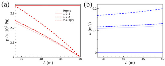
Figure 20.
(a,b), respectively, show the pressure and speed profiles in the channels on level 2 when the outlet of channel 1-2-1 is closed but other channels are open. For comparison, we plot the profiles of a homogeneous and open fracture network as light lines.
5. Discussion and Conclusions
Fluid migration plays an important role in the oil accumulation mechanism and hence is key to oil exploration. It has been widely accepted that fractures are oil migration pathways and the main controlling factor for oil accumulation in faulted basins [40,41]. The main contribution of this work is establishing a validated model by combining 1D Navier–Stokes equations and linear elastic equations to simulate the upward fluid flow in the structural fractures. Considering the relationship between the temperature and the oil viscosity, we also coupled the model with the energy equations describing the thermal process in the fractures.
Using the model, we have investigated the fluid migration and thermal process layer-by-layer for a single fracture, a bifurcated fracture, and a fracture network. Our results suggest that the parameters of both the fluid (Figure 5 and Figure 9) and the surrounding rock matrix (Figure 6 and Figure 8) affect the upward flow in the fractures. The outlet boundary condition is also very important. In good agreement with the experimental study by Yuan et al. [26], we found that the upward flow in an open fracture is mainly driven by the pressure difference between the inlet and outlet (Figure 4), so the fluid flow becomes a Darcy flow with a much lower speed in a closed fracture (Figure 7). As a result, the permeability is a more important factor affecting the profiles of the pressure and speed in a closed fracture (Figure 8(c1,c2)), compared with the profile in an open one (Figure 8(b1,b2)). Moreover, the liquid temperature in the closed fracture becomes closer to the rock matrix temperature as it gets closer to the outlet (Figure 7d), while the liquid temperature in the open fracture is basically maintained at the inlet temperature (Figure 4d).
For the bifurcated fracture, we focused on the influences of fracture division, and the heterogeneity from the main channel to the branches on the upward flow. We found that the fracture division reduces the pressure in the main channel connected to the entrance of the whole fracture (Figure 18b), but increases the pressure gradient and the fluid speed there (Figure 18c), which agrees well with the findings of Dana et al. [29]. The heterogeneity of the parameters between the main channel and the branches and between the branches has similar influences on the main channel but may affect the branches in opposite ways. As an example, for the flow in the main channel, decreasing the rock stiffness, either from the main channel to the branches or from one branch to the other, reduces its interior pressure but increases its speed. However, decreasing the stiffness from the main channel to the branches increases the outlet speed of both branches, while decreasing the stiffness from one branch to the other reduces the outlet speed of the branch with the higher stiffness. (Figure 12). In addition, we analyzed the influence of a closed branch on the upward flow in the whole bifurcated fractures (Figure 16), and found that closing a branch leads to a decrease in the internal pressure of the other branch channel as well as the main channel, an increase in the velocity of the main channel, and a decrease in the velocity of the other branch channel. Our result agrees well with those of Chen et al. [42], who pointed out that the blockage of small fractures may have a significant impact on the local velocity field, increasing the flow velocity in the main channel, but it may also have the opposite effect on the channel velocity on the same line.
Applying our model to the fracture network, we found that, with the increasing level of the network, the main contribution of the pressure difference shifts toward the entrance (Figure 18b), and the closer it is to the entrance, the greater is the speed of the fluid (Figure 18c). This finding highlights that the increased complexity of the network reduces the effective region for the pressure gradients to drive fluids upward from the entrance into the outlet. More importantly, we evaluated the effect of the parameter and boundary condition changing in a branch on the other branches, finding that the change has a greater impact on closer branches (Figure 19 and Figure 20).
The thermodynamic study of the upward flow of viscous fluid in vertical migration network channels can provide a reference for the dynamic prediction of oil exploration, and production. However, the structural fracture morphology of a real rock matrix is very complex. Both asymmetric bifurcation fault structures and non-uniform bifurcation fault structures may occur. Even if the complexity and non-uniformity are taken into account in our model, there will still be some prediction errors with the reality. Therefore, in order to achieve a more accurate simulation of oil upward migration, the model can be combined with microseismic monitoring to fit the actual fracture morphology [43,44]. Then, more accurate simulation results can be obtained by modeling and analyzing the real tree-shaped fracture network. Another important influencing factor that may not be considered in the current model is the fracture growth angle. Fracture inclination will affect the deformation, stress field, fracture mechanism, and displacement of a fractured rock matrix, change the stress magnitude and distribution of rock blocks, and affect the initiation and propagation of fractures [45]. At present, there are insufficient modeling studies and experimental observations on similar analysis of oil movement, and enough detailed parameter information is needed to make a direct comparison with this study. However, the developed model can provide detailed insights into both elastic matrix migration and fracture fractal characteristics of oil. It also sheds light on crucial variables for future characterization efforts, while providing useful information for legal and regulatory frameworks designed for oil exploration and extraction.
Author Contributions
Z.Q. and Y.L. established the flow field model, wrote the code, performed reliability verification, processed the data of the flow field, and analyzed the results. H.L. reviewed the paper and supervised the work, J.M. and S.Z. provided the literature review and participated in the writing of the manuscript. All authors have read and agreed to the published version of the manuscript.
Funding
This study is supported by the National Natural Science Foundation of China (Grant No. 12172094) and the Innovation and Entrepreneurship Training Program for College Students of China (Grant No. S202210593404).
Institutional Review Board Statement
Not applicable.
Informed Consent Statement
Not applicable.
Data Availability Statement
The raw data supporting the conclusions of this article will be made available by the authors on request.
Conflicts of Interest
The authors declare no conflicts of interest.
Appendix A. The Discretization of Our Governing Equation
Combining Equation (17) to Equation (9), we obtain the following governing equation describing the evolution of the pressure in a single fracture,
Applying an implicit time-stepping scheme and the standard second-order central difference method, we discretize Equation (A1) as
where is the temporal interval, n and represent the time steps, is the grid size, and , m and are the grid cell node numbers of the i channel. For example, channel 0 is characterized by a function . This channel length is 50 m and is 0.5 m. In this case, m is 100. The channel has m + 1 (101) nodes numbers. Node numbers are ,, …, . equals and equals . In the computation, we arrange Equation (A2) and update the pressure using the Thomas algorithm [46].
References
- Zou, C.; Zhai, G.; Zhang, G.; Wang, H.; Zhang, G.; Li, J.; Wang, Z.; Wen, Z.; Ma, F.; Liang, Y.; et al. Formation, distribution, potential and prediction of global conventional and unconventional hydrocarbon resources. Shiyou Kantan Kaifa/Petroleum Explor. Dev. 2015, 42, 13–25. [Google Scholar] [CrossRef]
- Sieminski, A. EIA Overview; Energy Information Administration: Washington, DC, USA, 2016.
- Gas transport and storage capacity in shale gas reservoirs—A review. Part A: Transport processes. J. Unconv. Oil Gas Resour. 2015, 12, 87–122. [CrossRef]
- Jiang, Q.; Cui, J.; Feng, X.T.; Zhang, Y.H.; Zhang, M.Z.; Zhong, S.; Ran, S.G. Demonstration of spatial anisotropic deformation properties for jointed rock mass by an analytical deformation tensor. Comput. Geotech. 2017, 88, 111–128. [Google Scholar] [CrossRef]
- Zhou, T.; Zhu, J.; Xie, H. Mechanical and Volumetric Fracturing Behaviour of Three-Dimensional Printing Rock-like Samples Under Dynamic Loading. Rock Mech. Rock Eng. 2020, 53, 2855–2864. [Google Scholar] [CrossRef]
- Zhang, S.; Yan, J.; Cai, J.; Zhu, X.; Hu, Q.; Wang, M.; Geng, B.; Zhong, G. Fracture characteristics and logging identification of lacustrine shale in the Jiyang Depression, Bohai Bay Basin, Eastern China. Mar. Pet. Geol. 2021, 132, 105192. [Google Scholar] [CrossRef]
- Gong, L.; Wang, J.; Gao, S.; Fu, X.; Liu, B.; Miao, F.; Zhou, X.; Meng, Q. Characterization, controlling factors and evolution of fracture effectiveness in shale oil reservoirs. J. Pet. Sci. Eng. 2021, 203, 108655. [Google Scholar] [CrossRef]
- Ogata, K.; Senger, K.; Braathen, A.; Tveranger, J. Fracture corridors as seal-bypass systems in siliciclastic reservoir-cap rock successions: Field-based insights from the Jurassic Entrada Formation (SE Utah, USA). J. Struct. Geol. 2014, 66, 162–187. [Google Scholar] [CrossRef]
- Wang, X.; Zhou, X.; Li, S.; Zhang, N.; Ji, L.; Lu, H. Mechanism Study of Hydrocarbon Differential Distribution Controlled by the Activity of Growing Faults in Faulted Basins: Case Study of Paleogene in the Wang Guantun Area, Bohai Bay Basin, China. Lithosphere 2022, 2022, 7115985. [Google Scholar] [CrossRef]
- Cartwright, J.; Huuse, M.; Aplin, A. Seal bypass systems. Am. Assoc. Pet. Geol. Bull. 2007, 91, 1141–1166. [Google Scholar] [CrossRef]
- Cartwright, J.; Santamarina, C. Seismic characteristics of fluid escape pipes in sedimentary basins: Implications for pipe genesis. Mar. Pet. Geol. 2015, 65, 126–140. [Google Scholar] [CrossRef]
- Oda, M. An equivalent continuum model for coupled stress and fluid flow analysis in jointed rock masses. Water Resour. Res. 1986, 22, 1845–1856. [Google Scholar] [CrossRef]
- Chaudhary, A.S.; Ehlig-Economides, C.; Wattenbarger, R. Shale oil production performance from a stimulated reservoir volume. In Proceedings of the SPE Annual Technical Conference and Exhibition, Denver, CO, USA, 30 October–2 November 2011; OnePetro: Richardson, TX, USA, 2011. [Google Scholar]
- Agboada, D.K.; Ahmadi, M. Production decline and numerical simulation model analysis of the Eagle Ford Shale oil play. In Proceedings of the SPE Western Regional & AAPG Pacific Section Meeting 2013 Joint Technical Conference, Monterey, CA, USA, 19–25 April 2013; OnePetro: Richardson, TX, USA, 2013. [Google Scholar]
- Karimi-Fard, M.; Durlofsky, L.J.; Aziz, K. An efficient discrete-fracture model applicable for general-purpose reservoir simulators. SPE J. 2004, 9, 227–236. [Google Scholar] [CrossRef]
- Jiang, J.; Younis, R.M. Hybrid coupled discrete-fracture/matrix and multicontinuum models for unconventional-reservoir simulation. SPE J. 2016, 21, 1009–1027. [Google Scholar] [CrossRef]
- Wu, Y.s.; Wang, C.; Li, J.; Fakcharoenphol, P. Transient Gas Flow in Unconventional Gas Reservoir. SPE Annu. 2012, 4–7. [Google Scholar]
- Liu, Y.; Guo, J.; Chen, Z. Leakoff characteristics and an equivalent leakoff coefficient in fractured tight gas reservoirs. J. Nat. Gas Sci. Eng. 2016, 31, 603–611. [Google Scholar] [CrossRef]
- Xu, W.; Thiercelin, M.; Ganguly, U.; Weng, X.; Gu, H.; Onda, H.; Sun, J.; Le Calvez, J. Wiremesh: A novel shale fracturing simulator. In Proceedings of the International Oil and Gas Conference and Exhibition in China, Beijing, China, 8–10 June 2010; OnePetro: Richardson, TX, USA, 2010. [Google Scholar]
- Weng, X.; Kresse, O.; Cohen, C.; Wu, R.; Gu, H. Modeling of hydraulic-fracture-network propagation in a naturally fractured formation. SPE Prod. Oper. 2011, 26, 368–380. [Google Scholar]
- Geng, L.; Li, G.; Wang, M.; Li, Y.; Tian, S.; Pang, W.; Lyu, Z. A fractal production prediction model for shale gas reservoirs. J. Nat. Gas Sci. Eng. 2018, 55, 354–367. [Google Scholar] [CrossRef]
- Zhang, L.; Cui, C.; Ma, X.; Sun, Z.; Liu, F.; Zhang, K. A fractal discrete fracture network model for history matching of naturally fractured reservoirs. Fractals 2019, 27, 1940008. [Google Scholar] [CrossRef]
- Ozdemirtas, M.; Babadagli, T.; Kuru, E. Experimental and numerical investigations of borehole ballooning in rough fractures. SPE Drill. Complet. 2009, 24, 256–265. [Google Scholar] [CrossRef]
- Lai, C.Y.; Zheng, Z.; Dressaire, E.; Wexler, J.S.; Stone, H.A. Experimental study on penny-shaped fluid-driven cracks in an elastic matrix. Proc. R. Soc. Math. Phys. Eng. Sci. 2015, 471, 2182. [Google Scholar] [CrossRef]
- Leythaeuser, D.; Schaefer, R.G.; Yukler, A. Role of diffusion in primary migration of hydrocarbons. AAPG Bull. 1982, 66, 408–429. [Google Scholar]
- Yuan, L.; Zhou, F.; Li, B.; Gao, J.; Yang, X.; Cheng, J.; Wang, J. Experimental study on the effect of fracture surface morphology on plugging efficiency during temporary plugging and diverting fracturing. J. Nat. Gas Sci. Eng. 2020, 81, 103459. [Google Scholar] [CrossRef]
- Li, M.; Zhou, F.; Sun, Z.; Dong, E.; Zhuang, X.; Yuan, L.; Wang, B. Experimental study on plugging performance and diverted fracture geometry during different temporary plugging and diverting fracturing in Jimusar shale. J. Pet. Sci. Eng. 2022, 215, 110580. [Google Scholar] [CrossRef]
- Wang, B.; Zhou, F.; Wang, D.; Liang, T.; Yuan, L.; Hu, J. Numerical simulation on near-wellbore temporary plugging and diverting during refracturing using XFEM-Based CZM. J. Nat. Gas Sci. Eng. 2018, 55, 368–381. [Google Scholar] [CrossRef]
- Dana, A.; Peng, G.G.; Stone, H.A.; Huppert, H.E.; Ramon, G.Z. Backflow from a model fracture network: An asymptotic investigation. J. Fluid Mech. 2019, 864, 899–924. [Google Scholar] [CrossRef]
- Guo, J.; Liu, Y. A comprehensive model for simulating fracturing fluid leakoff in natural fractures. J. Nat. Gas Sci. Eng. 2014, 21, 977–985. [Google Scholar] [CrossRef]
- Biot, M.A.; Masse, L.; Medlin, W.L. Temperature analysis in hydraulic fracturing. J. Pet. Technol. 1987, 39, 1389–1397. [Google Scholar] [CrossRef]
- Kamphuis, H.; Davies, D.R.; Roodhart, L. A new simulator for the calculation of the in situ temperature profile during well stimulation fracturing treatments. J. Can. Pet. Technol. 1993, 32. [Google Scholar] [CrossRef]
- Wenzheng, L.; Qingdong, Z.; Jun, Y. Numerical simulation of elasto-plastic hydraulic fracture propagation in deep reservoir coupled with temperature field. J. Pet. Sci. Eng. 2018, 171, 115–126. [Google Scholar]
- Whitsitt, N.F.; Dysart, G.R. The effect of temperature on stimulation design. J. Pet. Technol. 1970, 22, 493–502. [Google Scholar] [CrossRef]
- Kovalyshen, Y.; Detournay, E. A reexamination of the classical PKN model of hydraulic fracture. Transp. Porous Media 2010, 81, 317–339. [Google Scholar] [CrossRef]
- Lu, C.; Jiang, H.; Qu, S.; Zhang, M.; He, J.; Xiao, K.; Yang, H.; Yang, J.; Li, J. Hydraulic fracturing design for shale oils based on sweet spot mapping: A case study of the Jimusar formation in China. J. Pet. Sci. Eng. 2022, 214, 110568. [Google Scholar] [CrossRef]
- Zhi, D.; Xiang, B.; Zhou, N.; Li, E.; Zhang, C.; Wang, Y.; Cao, J. Contrasting shale oil accumulation in the upper and lower sweet spots of the lacustrine Permian Lucaogou Formation, Junggar Basin, China. Mar. Pet. Geol. 2023, 150, 106178. [Google Scholar] [CrossRef]
- Wang, Y.; Li, T.; Chen, Y.; Ma, G. A three-dimensional thermo-hydro-mechanical coupled model for enhanced geothermal systems (EGS) embedded with discrete fracture networks. Comput. Methods Appl. Mech. Eng. 2019, 356, 465–489. [Google Scholar] [CrossRef]
- Detournay, E.; Garagash, D.I. The near-tip region of a fluid-driven fracture propagating in a permeable elastic solid. J. Fluid Mech. 2003, 494, 1–32. [Google Scholar] [CrossRef]
- Ma, C.; Dong, C.; Luan, G.; Lin, C.; Liu, X.; Elsworth, D. Types, characteristics and effects of natural fluid pressure fractures in shale: A case study of the Paleogene strata in Eastern China. Pet. Explor. Dev. 2016, 43, 634–643. [Google Scholar]
- Xu, S.; Hao, F.; Xu, C.; Zou, H.; Zhang, X.; Zong, Y.; Zhang, Y.; Cong, F. Hydrocarbon migration and accumulation in the northwestern Bozhong subbasin, Bohai Bay Basin, China. J. Pet. Sci. Eng. 2019, 172, 477–488. [Google Scholar] [CrossRef]
- Chen, X.; Zhao, J.; Chen, L. Experimental and numerical investigation of preferential flow in fractured network with clogging process. Math. Probl. Eng. 2014, 2014, 879189. [Google Scholar] [CrossRef]
- Wang, W.; Su, Y.; Zhang, X.; Sheng, G.; Ren, L. Analysis of the complex fracture flow in multiple fractured horizontal wells with the fractal tree-like network models. Fractals 2015, 23, 1550014. [Google Scholar] [CrossRef]
- Umar, I.A.; Negash, B.M.; Quainoo, A.K.; Ayoub, M.A. An outlook into recent advances on estimation of effective stimulated reservoir volume. J. Nat. Gas Sci. Eng. 2021, 88, 103822. [Google Scholar] [CrossRef]
- Feng, P.; Ma, H.; Qian, J.; Wang, J.; Cao, Y.; Ma, L.; Luo, Q. Influence of Bifurcated Fracture Angle on Mechanical Behavior of Rock Blocks. Indian Geotech. J. 2023, 53, 622–633. [Google Scholar] [CrossRef]
- LeVeque, R.; Oliger, J. Numerical methods based on additive splittings for hyperbolic partial differential equations. Math. Comput. 1983, 40, 469–497. [Google Scholar] [CrossRef]


Disclaimer/Publisher’s Note: The statements, opinions and data contained in all publications are solely those of the individual author(s) and contributor(s) and not of MDPI and/or the editor(s). MDPI and/or the editor(s) disclaim responsibility for any injury to people or property resulting from any ideas, methods, instructions or products referred to in the content. |
© 2024 by the authors. Licensee MDPI, Basel, Switzerland. This article is an open access article distributed under the terms and conditions of the Creative Commons Attribution (CC BY) license (https://creativecommons.org/licenses/by/4.0/).