1. Introduction
The use of unmanned aerial vehicle (UAV) swarms [
1,
2] has significantly expanded the range of applications and possibilities in the unmanned field, surpassing the capabilities of single-vehicle systems. Formation-based control algorithms aim to guide all vehicles to form specific configurations while maintaining relative velocity and distance. However, relying on fixed formation patterns limits the adaptability of formation control in different environments. Hence, the notion of dynamically altering configurations in UAV formation control has garnered significant attention from researchers, particularly the maneuver control for the purpose of achieving continuous formation change [
3,
4,
5,
6]. This approach possesses the ability to autonomously navigate aerial formations in cluttered and wild environments, effectively providing assistance during natural disasters like earthquakes and floods. Maneuver control can aid in formation search and guidance [
7]. Additionally, researchers can inspect restricted areas such as documenting structural and cultural artifacts within historical buildings [
8] or autonomously searching subterranean environments [
9], which can gain situational awareness and assist specialized personnel in specific missions, such as assessing the structural integrity of collapsed buildings, tunnels, mines, exploration of a newly discovered branch in a cave network, and searching for lost persons. Formation configurations can be associated with different tasks and environments, such as collective animal behavior [
10] in nature or reconnaissance and strike missions [
11,
12]. However, continuous configuration changes increase system complexity and communication requirements among UAV agents, particularly when adjusting and preserving the position and orientation of each agent in motion [
13]. Additionally, the effectiveness of configuration change may be hindered by various external and internal constraints.
Therefore, various methods combining formation control with configuration changes have been extended to multi-agent systems, resulting in more versatile forms of unmanned vehicles, including maneuvering [
13,
14], surveillance [
15], reconnaissance [
16], and traffic monitoring and management [
17]. In addition to researching practical constraints and scenarios, distributed methods have proven to be more adaptable and consider mutual autonomy coordination for configuration changes, in contrast to centralized approaches [
3,
17]. This suggests that the characteristics of the distributed strategy are better suited for the dynamic configuration changes of formations. Distributed formation control strategies closely related to configurations can be broadly categorized into position, displacement, and distance-based methods, based on the types of sensed and controlled variables used thus far. However, these methods have limited effectiveness in accurately tracking the target formation [
18], which restricts configuration changes to variations in time, scales, and orientation of the target configuration [
19,
20,
21]. From a control perspective, the dynamic change of configuration can be specified at the global formation level [
19,
20,
21,
22] or the local level [
23,
24]. The global approach involves presetting the path points of the formation’s center of gravity for agents to follow, maintaining the rigid body structure by preserving relative positions and transitioning between different formation shapes. On the other hand, the local approach focuses on agent-level control, which is more adaptable to tasks and collision avoidance. The first approach involves maintaining the rigid structure of the configuration with constant constraints, requiring a configuration with a predefined change scale and nominal configuration. Ref. [
6] proposed an affine-based generation method for target configuration using an interaction law with both designed positive and negative weights (different from consensus control law). Ref. [
22] extended the affine-based method by introducing a stress matrix to enable general linear transformations involving translation, rotation, scaling, shear, or compositions of these transformations. These methods ensure that the configuration maintains the rigid graph structure in each step, preserving collinearity and distance ratios, while also enabling maneuver control. The second approach is more adaptable, aiming to maximize the observation capabilities of the robot team and facilitate obstacle avoidance. This method focuses on actively moving mobile agents to improve the accuracy of target detection with a dynamically adjustable geometry. Ref. [
25] studied a formation loop that forms an un-rigid configuration using a distributed non-linear model predictive controller (DNMPC) and an estimator module. Ref. [
26] discussed the use of artificial potential fields (APF) as a cost function in a non-linear model predictive controller (NMPC) with a modified A* path planner method for configuration changes. These methods exhibit generality, allowing adaptation to both static and dynamic environments, where the value and direction of velocity can be adjusted based on the current cost.
However, these methods have limitations in terms of generality. The first method fails to address sudden changes in an agent’s velocity in terms of value and direction. The velocity is directly designed in each step of the configuration transformation, relying on prior information about the environment. The second approach heavily relies on strong communication interaction, which may lead to reconstruction failures in the event of breakdowns in one or more agents. Therefore, the goal of formation control with continuous configuration changes is to ensure low communication costs, an adaptable change model, as well as equilibrium and stability within the system.
Thus, this paper presents an algorithm that integrates APF-based leader control [
27,
28,
29,
30] with the affine formation, while utilizing behavior optimization for local trajectory calculation. This algorithm enables efficient navigation for multi-agents within a formation by incorporating artificial potentials to guide agent movement, a virtual leader for formation path planning, and geometric pattern modeling for obstacle avoidance. Moreover, the agents within the formation are initially placed randomly and are adjusted applying additional forces to move individual agents to their new equilibrium positions in various configurations.
The objective of employing potential functions is to guide agents away from obstacles and towards or away from the virtual leader, while also ensuring cohesion among agents as they navigate through the environment [
31,
32,
33]. In other words, the configuration of the formation can be adjusted based on the error in the velocity vector of agents and the virtual leader. Therefore, the potential functions used in our methodology consist of virtual leader forces and obstacle forces. As the virtual leader’s position moves, the artificial potential relationships guide the group along the path defined by the virtual leader’s motion. By relying on the global motion of a virtual leader, the complexity of planning multiple collision-free paths for numerous vehicles is reduced to planning just one collision-free path. Consequently, the interacting agents enter optimization procedures, where the explicit fourth-order Runge–Kutta methods [
34] are introduced into the local control law. This method is commonly used to solve ordinary differential equations (ODE) and estimates the value of the next step by utilizing the slope of the midpoint with truncation error O (
) in each step size. Subsequently, the local trajectory [
35] of each agent estimates the value of the function at the next step by calculating the slopes of multiple intermediate points to obtain the numerical solution.
The virtual leader abstraction is utilized to guide the formation through the environment. It is important to note that the virtual leader is not a physical vehicle, but an imaginary point used as a reference for the movement of the formation. The construction of the virtual leader is similar to Leonard [
3]. The virtual leader abstraction offers a significant advantage by eliminating the need for individual node trajectories, focusing solely on planning the path of the virtual leader through areas of interest for the entire team. This approach greatly reduces communication requirements. Additionally, the motion of the virtual leader is limited to a distance that prevents any of the vehicles from experiencing excessive total forces in the direction of the virtual leader’s motion.
Furthermore, the communication requirements among agents may vary depending on the level of precision needed for configuration changes. Each agent updates its trajectory within the formation based on the positions of other agents, obstacles, and the virtual leader each time step. The position of the virtual only needs to be transmitted to each agent once per update at most, regardless of whether there is a need to recalculate the position to adjust the local trajectory. This approach ensures that the bandwidth requirements for all agents interacting with their positions remain manageable in small formations (less than 20 agents), as it considers only horizontal motion consensus. However, for larger groups, the position information would be limited to agents within a nearby radius.
This paper investigates the generality of formation-desired configurations and proposes an adaptable algorithm for local trajectory planning. The algorithm ensures the continuous change of geometric patterns and improves the consistency of local trajectory planning with realistic constraints. Consequently, the formation control relies less on prior information and enhances the ability to avoid obstacles and other agents in real-time, particularly in situations involving sudden obstacles. Additionally, the combination of formation control methods and optimal techniques expands the utilization of formation configuration variations and definitions to adapt to more complex environments.
The contributions of this article could be summarized as follows:
A novel non-linear and dynamical system for formation configurations changing is created by the combination of the global and local control law, which could relieve the dependence on the rigid body of formation.
An APF-based adjustment metric is developed for local trajectory planning through various forces. It could solve the problem of local minimum value of APF and update the local navigation to filter the discrete value due to a sudden change of velocity.
A novel optimal framework has been integrated, combining a virtual leader to consider dynamic feasibility, obstacle avoidance, and flexibility. This framework can improve the elasticity of configuration variations in potential collision.
The paper is organized as follows.
Section 2 describes the preliminaries. In
Section 3, the description of the interaction forces among agents, virtual leader, and obstacles is presented. The description and proof of the main results for local control laws are given in
Section 4. The results of the simulation and discussions are drawn in
Section 5.
Section 6 concludes the entire paper and provides a glimpse into future prospects.
2. Preliminaries
This section mainly introduces the preliminary knowledge of unmanned aerial vehicles, containing graph theory to depict the inner relationship of the system and the state–space equation of the UAV system.
2.1. Graph Theory
A weighted undirected graph is denoted as , where represents the set of all vertices in the undirected graph, and each vertex represents an agent. represents the edge set between vertices, and represents the edge from vertex to vertex; an edge connection between two vertices indicates that there is an information interaction between these two vertices. The graph is undirected if it allows two-way communication; otherwise, it is directed. represents the adjacency matrix indicating the relationship between agents, where is the weight of the side and where the diagonal elements of the matrix are all 0. For , if the agents and can receive information from each other, then the elements in the adjacency matrix are ; otherwise, the element in the adjacency matrix is 0. This paper has only considered an undirected graph, in which .
2.2. Kinematic and Dynamic Models of UAV
The multi-agent formation is denoted as , where the vertex within graph is mapped to point . In addition, it is assumed that the first agents are leaders and the rest are followers. Let and be the sets of leaders and followers, respectively, where .
A mass-point [
18,
36] can be used to describe the UAV agent and the motion of the formation. The fixed-wing agent model is described as
Figure 1 shows:
It is shown that all these variables are presented to depict the agent motion from the inertial coordinate frame
; thus, the kinematic motion equations for UAV can be expressed as
Meanwhile, the dynamic of UAV is given by
where
and
are the range displacement projected on the
and
axes separately,
is the flight altitude, and
is the speed which is assumed as ground speed in the paper,
and
are the heading angle and the flight one.
is the engine thrust vector directed with the velocity vector,
is a general term for drag. Additionally,
is used to describe the gravity of the agent, the
load
is contained by an elevator,
the banking angle and the engine thrust
are considered as the control inputs.
Therefore, by the use of the feedback linearization technology, the non-linear UAV model Formulation (1) and (2) can be simplified to a linear constant system
However,
,
, and
are virtual control inputs to describe the accelerations in each way. The actual control input is given as
where the heading angle
can be expressed as
, the fight one
is
. Thus, in terms of the state–space representation, denoting
,
, and
, which are the position, velocity, and acceleration control vector, the double-integrator system is reduced as
where
,
,
. Consider a flock of
agents in
and
as the position of agent
and
is the configuration of all the agents, where
and
. Let
be the number of edges in an undirected graph and the orientation of which is the direction assignment to each edge.
Given the substantial difference in time constants between the horizontal and vertical trajectory controllers, configuration control can be concentrated primarily on achieving consensus in the horizontal positional and velocity motion. Meanwhile, the control input is composed of anticipated configuration, reference trajectory, velocity, and state information of adjacent entities.
It is presupposed that all followers possess a restricted situational awareness, and their capability to detect fellows is constrained by their sensing range. Supposing all Unmanned Aerial Vehicles (abbreviated as UAV) possess an equivalent efficacious sensing range, thus the neighbor set of agent
can be depicted as:
where
is the position vector from UAV
to UAV
,
is the Euclidean norm,
is the sensing range.
Let denote the artificial potential between UAV and , and are sensing range and desired distance, respectively. is the Kronecker product and as the Euclidean norm of vector notation, is the identity matrix of order , and is the dimension of a linear space. For any vector , denotes the diagonal matrix whose diagonal entry is the entry of . denotes the total artificial potential of UAV .
2.3. Affine Transformation Description
Based on the undirected graph
to describe the communication topology of multi-agent formation, denote the
as the nominal configuration and let
be the affine span. Let the dimension be
and
in
be the affine image set and the associated definitions and lemmas about affine transformation are presented as follow [
22].
Definitions 1 (Affine Span). A linear space can be obtained by any affine span. Thus, provided with the nominal configuration for formation , the affine span is: Lemma 1 (Affine Span with Rank condition). The nominal configuration affinely span if and only if and , where .
Definitions 2 (Affine Image). The affine image set consisting of all the affine transformations of the nominal configuration , which is defined as follows:where is the predefined affine image and can be applied to all time-varying target configurations, and a linear subspace because it is closed under addition and scalar multiplication, and are the linear affine transformation. Lemma 2 (General Rigid). The nominal configuration is universally rigid if and only if the stress matrix is positive semi-definite and satisfies .
Definitions 3 (Stress Matrix). The stress matrix can be viewed as generalized graph Laplacian matrices with both positive and negative edge weights. Let graph stress denote as the scalar , represents the attractive force and the opposite, and denote if:the equilibrium set satisfies: Equation (10) can be expressed in a matrix form as
, denote the
:
Definitions 4 (Affine Localizability). Denote the nominal formation as affinely localizable if and only if affinely span (Lemma 1) and any , can be uniquely determined by .
Lemma 3 (Affine Localizability of Nominal Formation). If the nominal configuration affinely span and is positive semi-definite, is affinely localizable if and only if is nonsingular.
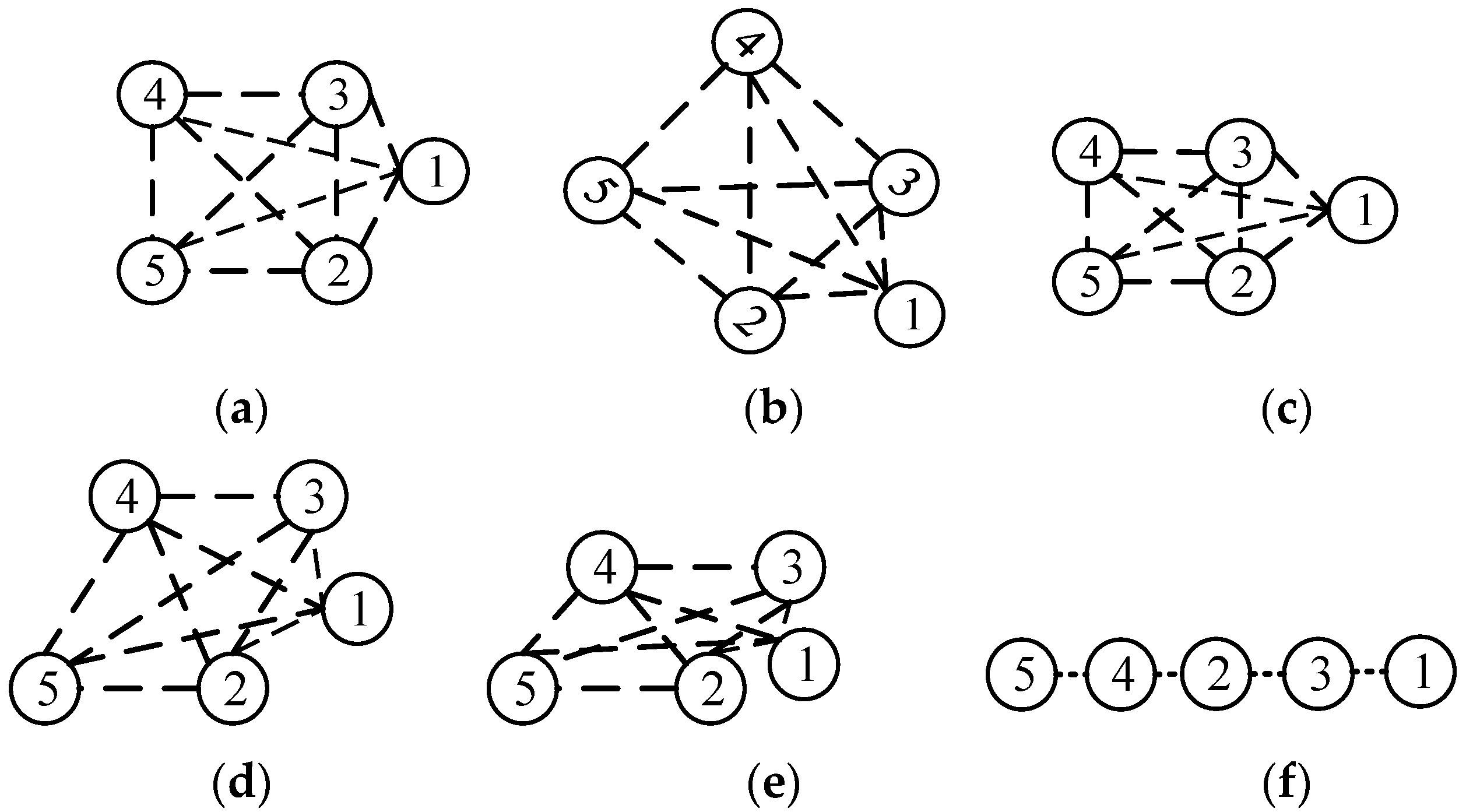
From
Figure 2, it can be seen that
Figure 2b–d are obtained by rotating, scaling, and shearing the original formation
Figure 2a, respectively.
Figure 2e is obtained from
Figure 2d by reducing the scale in the vertical direction.
Figure 2f, where the four points are collinear, is obtained from
Figure 2e by reducing the scale in the vertical direction to zero.
Due to the simplification of the communication complexity, only leaders need to be aware of the affine transformation and controlled only. Thus, the leader–follower strategy can be well adopted as the control law, and the leaders’ positions will have a one-to-one correspondence to the affine transformation .
5. Simulation and Analysis
In this section, we proceed to conduct numerical simulations to illustrate the theoretical results and validate the effectiveness of the novel formation control algorithm.
The whole experimental process is shown in
Figure 6, and the algorithm in two-dimensional is described as follows:
The randomly distributed generated agents denoted as , are steered to rendezvous and make a swarm formation as the nominal configuration . The leaders are set and then time-varying velocity (10) starts to change in this stage for all agents (20).
Desired geometric patterns are predefined and generated with desired trajectories and corresponding positions of the formation based on the knowledge of obstacle position and shape available.
A trajectory through all the barycenter of leaders of each predefined configuration; thus, this virtual agent motives with constant velocity in a single-integrator differentiable.
Based on the available knowledge of obstacles, using constant interaction with other agents and obstacle constraints (20) to trigger local trajectory planning in Algorithm 1 (15) and (16).
The formation operated the (20) control law to adjust the trajectories of agents possibly entering collide zones of obstacles while changing the configuration of formation , which can demonstrate the tracking ability of the algorithm (21).
It is noted that only the leaders possess global information regarding the desired trajectory (). The focus on the position error relative to the reference trajectory is solely on the leaders. Consequently, the control laws for the leaders are not explicitly designed in this paper.
In order to evaluate the performance of our proposed methods, all the experiments are simulated on PC with MATLAB R2020a Windows 10. Protocol (20) is used to steer seven UAV agents moving in a two-dimensional space with five processes above through Algorithms 1 and 2.
The number of agents , the sensing range , desired distance from the virtual leader , obstacles radius , maximum velocity , max acceleration , max velocity error , max trajectory error , the timestep . Other parameters were set as , , , , . All the above parameters remained fixed throughout the simulation.
The experiment is divided into three phases: Firstly, the desired path of the formation, the position of configuration, and the obstacles are pre-defined. The experiment could be conducted by affine maneuvering by single-integrator control law from (20) in Zhao [
22]. Secondly, the obstacle is randomly located in the trajectory of formation to test the effect of a local trajectory planning method (Algorithm 1). Finally, the formation with seven agents is operated as Algorithm 2 and the experiment process acts as
Figure 6.
5.1. Phase I
With the available information regarding obstacles, it becomes feasible to pre-define the desired path and its corresponding configuration. The purpose of this part is to generate the nominal configurations during each time interval, which can provide the desired path for the leaders of the formation and the desired tracking velocity. The positions of agents are randomly selected from the box
, as
Figure 7b shows. Their velocities of leaders are set as constant
and directions in intervals
. Agents 1, 2, and 3 are assigned as leaders illustrated in red through the whole simulation and the four change forms of configuration are calculated, scaling, rotation, shear, and translation. It is shown that the affine-based leader/follower consensus protocol can form the continuous configuration change for the formation. The nominal configuration is established prior to 6 s. At the moment
and
the formation is expected to undergo scaling in the y-direction, with shrinking and enlargement occurring, respectively. Starting from
and
, the formation initiates rotation. Additionally, there is shearing at
and
, while the formation translates during other time intervals within the given range.
One can see that the velocity for followers would have suddenly changed to meet the requirement in each time interval of the different configuration changes. The scale of change could not be controlled effectively in any case.
5.2. Phase II
The aim of the second part is mainly to test the effect of the algorithm of local trajectory planning. The position of the obstacle is located randomly at
(x, y, width, height) and agents are from the box
as
Figure 8a shows; the acceleration, velocity, and the angle of drift are in intervals
,
and
, the velocity of the virtual leader is
. The formation has started at the nominal configuration and encounters the obstacle along the desired path
, as
Figure 8b shows. The state
of the virtual leader is the desired state for agents, as
Figure 8b shows, and the formation would generate Algorithm 1 to steer agents to avoid obstacles. The velocity and its error related to the virtual leader are given in
Figure 8c,d; as can been seen, the velocity fluctuates greater at
and
moving through the obstacle and the velocity change interval is from
to
.
Figure 8d illustrates the change in velocity error during the same time interval. The primary reason for this is that the desired trajectory, as moved by the virtual leader, would directly pass through the obstacle. However, the formation manages to avoid collision and maintain its configuration due to the forces exerted by the virtual leader. In
Figure 8e, the trajectory error of all agents is depicted, with the note that the X and Y axes have different scales. It can be observed that the leaders and followers exhibit smaller average position errors, while the overall formation has a relatively larger error. The desired trajectory is not fully matched due to the influence of uninformed followers on the leaders, but it remains within an acceptable range. Lastly,
Figure 8f demonstrates the total velocity error for all agents, indicating that the protocol will converge eventually.
5.3. Phase III
The purpose of this part is to test the affine-based local trajectory planning algorithm in the pre-defined positions of obstacles to follow the desired path without collision. The positions of three obstacles are located at
,
, and
. The initial velocity of the virtual leader is set
and it moves with constant velocity through all the paths with direction intervals
. Meanwhile, based on the velocity of the virtual leader
, the velocities of agents in the formation are randomly generated with a standard normal distribution. The initial acceleration of the agents is set
. The formation starts at the random positions
to follow the desired path
, planning the local trajectory. From
Figure 9a, it is known that all the accelerations of agents have changed drastically and unpredictably, especially in the interval of
, and would converge in the final. The main reason is that input of agents would increase or decrease suddenly when the forces among agents undergo changes.
Figure 9b depicts the velocity error of the agents, indicating that the reference velocity is well tracked by both leaders and followers throughout the trajectory tracking process. The experimental results particularly demonstrate that the proposed algorithm enables the asymptotic tracking of the desired trajectory and remains effective even when the trajectory changes suddenly due to the formation steering local planning to avoid collisions during the motion process.
Figure 9c illustrates that the minimum distance between agents consistently remains greater than 0, indicating successful collision avoidance for the formation and the maintenance of the desired configuration within the acceptable error range. Additionally,
Figure 9d indicates that trajectory tracking is achieved satisfactorily.
5.4. Discussion
The experiments primarily focused on determining the optimal trajectory of each agent for affine maneuver control, revealing that a single mode of control may lack generality in complex environments to some extent. The proposed algorithm has been validated to be effective, particularly in addressing situations involving colliding obstacles. From the experiments, it was observed that each agent in the swarm autonomously carried out obstacles’ detection, judgment, and decision-making, compared with the original algorithm. The virtual leader mainly influenced an agent if it was likely to enter the zone where obstacles react, while the other agents continued to track desired trajectories with less effect from the virtual leader forces and reach predefined positions. Notably, even in the presence of abrupt changes in trajectories or obstacles, the proposed algorithm remained effective.
From
Figure 7,
Figure 8 and
Figure 9, it is demonstrated that the purpose of the proposed algorithm is to guarantee the configuration change to avoid the collision autonomously and maneuver continuously to track the predefined trajectory of an affine image set
. Thus,
Figure 7b shows that the random formation is generated at the beginning and starts to form the nominal configuration and then reach each
(
from
). However, a pre-defined trajectory would not avoid the obstacles effectively and could not provide the capability of changing velocity
suddenly.
Therefore, the proposed model is introduced to deal with the problem. It is shown that 11 desired positions have been pre-defined in
Figure 7, and the original path shows the possibility of collision. Note that system of detecting and steering each agent is determined by distance
only. In any case, the formation steered by an affine-based maneuvering method would fall apart and lose the body integrity when encountering the obstacles. Moreover, a virtual leader is designed to operate based on the pre-defined trajectory of the centroid of the pre-defined configurations as
Figure 3 demonstrates, denoted as
(12).
The advantage of this virtual strategy lies in its ability to enhance system functionality without significantly increasing complexity. Firstly, this strategy does not interfere with the formation motion. Secondly, the trajectory of the virtual agent is constructed based on the existing pre-defined trajectory. Lastly, this virtual agent can be seamlessly integrated into the control protocol, serving as an adjustment metric. Thus, the virtual leader introduced into the algorithm can modify the formation motion and improve the effectiveness of formation maneuvering.
In order to evaluate the effectiveness of the proposed method, we use two indexes to evaluate the motion results.
Table 1 intuitively shows the average value of all the experimental results with motion speed and track accuracy. It can been seen from
Table 1 that the proposed method had the highest accuracy value. However, the time has been taken larger than that of the affine-based maneuvering method, which is due to the complexity of the proposed being higher than the affine-based maneuvering method (
and
).
The second term Speed shows that the affine-based maneuvering took up 40 s, and the proposed method used 450 s. Obviously, the proposed method would use more time than the classic one with higher computational cost. Firstly, based on (22), the classic method basically solved the changeable problem of formation configurations for multi-agent. Then, the proposed method took more within each time step due to the calculation from Algorithm 1 (15).
The obstacle added to the experiment scenario is depicted in
Figure 10a, which is based on
Figure 7a. As illustrated in
Figure 7b, the new obstacle is inserted between
to
. The experimental results primarily focus on the formation maneuvering
and are obtained as follows.
It has been shown that the proposed method improves the maneuvering ability of the formation. From
Figure 10b, it is evident that the trajectory error is reduced by the proposed method. Furthermore, the velocity of the X axis in the classic method undergoes more drastic changes compared to the proposed method, as observed in
Figure 10c,e. Similarly,
Figure 10d,f demonstrate that the velocity of the Y axis in the proposed method changes smoothly.
6. Conclusions
The changes in formation configuration have been confirmed to be feasible. However, the challenge of maneuvering the formation while avoiding obstacles and converging to desired values has not been adequately addressed to enhance practical application. Moreover, the concept of a rigid body may not suffice in diverse environmental situations. Although the affine technique has somewhat resolved this issue by continuously providing multiple geometric patterns for configuration changes, it requires an adjustable environment and the maintenance of a rigid body at all times. As a result, this method lacks some generality for practical application, particularly in complex environments.
Therefore, this paper introduces a new consensus protocol based on a hybrid control model to enhance the effectiveness of formation maneuver control and obstacle avoidance in complex environments. The protocol employs distributed control laws with a virtual leader for double-integrator control and establishes the system’s stability. The presented algorithm showcases the capability to autonomously adjust each local trajectory of a formation based on potential forces when encountering obstacle colliding zones. Crucially, the control law is confined to each agent’s local reference frame, thereby improving the adaptability and scalability of the formation in realistic environments. Furthermore, the results show that the formation, steered by the proposed control algorithm, can still reach the predefined configuration even in the presence of violent trajectory changes. Additionally, the algorithm effectively reduces communication consumption.
In the future, there are several important topics that require attention. These include investigating more intricate graph structures, dynamic leader reassignment, and transitioning between distributed and decentralized control laws to enhance autonomy. Moreover, it is crucial to develop more autonomous control laws for adapting to environmental changes, improve deep learning techniques to establish rule-based response mechanisms, explore the interconnections between agents in complex networks, utilize the MPC method for local environment prediction, and delve into other related areas.


